Prevalence of Pure Versus Mixed Snow Cover Pixels across Spatial Resolutions in Alpine Environments

Selkowitz, David J.; Forster, Richard R.; Caldwell, Megan K.

doi:10.3390/rs61212478

Open AccessArticle

Prevalence of Pure Versus Mixed Snow Cover Pixels across Spatial Resolutions in Alpine Environments

by

David J. Selkowitz

^1,2,*,

Richard R. Forster

² and

Megan K. Caldwell

^3,4

¹

US Geological Survey, Alaska Science Center, 4210 University Drive, Anchorage, AK 99508, USA

²

Department of Geography, University of Utah, 260 S. Central Campus Dr., Room 270, Salt Lake City, UT 84112–9155, USA

³

US Geological Survey, Geosciences and Environmental Change Science Center, P.O. Box 25046, DFC, MS 980, Denver, CO 80225, USA

⁴

Department of Ecology and Evolutionary Biology, University of Colorado, Campus Box 334, Boulder, CO 80339–0334, USA

^*

Author to whom correspondence should be addressed.

Remote Sens. 2014, 6(12), 12478-12508; https://0-doi-org.brum.beds.ac.uk/10.3390/rs61212478

Submission received: 2 October 2014 / Revised: 29 November 2014 / Accepted: 1 December 2014 / Published: 11 December 2014

Download

Browse Figures

Versions Notes

Abstract

:

Remote sensing of snow-covered area (SCA) can be binary (indicating the presence/absence of snow cover at each pixel) or fractional (indicating the fraction of each pixel covered by snow). Fractional SCA mapping provides more information than binary SCA, but is more difficult to implement and may not be feasible with all types of remote sensing data. The utility of fractional SCA mapping relative to binary SCA mapping varies with the intended application as well as by spatial resolution, temporal resolution and period of interest, and climate. We quantified the frequency of occurrence of partially snow-covered (mixed) pixels at spatial resolutions between 1 m and 500 m over five dates at two study areas in the western U.S., using 0.5 m binary SCA maps derived from high spatial resolution imagery aggregated to fractional SCA at coarser spatial resolutions. In addition, we used in situ monitoring to estimate the frequency of partially snow-covered conditions for the period September 2013–August 2014 at 10 60-m grid cell footprints at two study areas with continental snow climates. Results from the image analysis indicate that at 40 m, slightly above the nominal spatial resolution of Landsat, mixed pixels accounted for 25%–93% of total pixels, while at 500 m, the nominal spatial resolution of MODIS bands used for snow cover mapping, mixed pixels accounted for 67%–100% of total pixels. Mixed pixels occurred more commonly at the continental snow climate site than at the maritime snow climate site. The in situ data indicate that some snow cover was present between 186 and 303 days, and partial snow cover conditions occurred on 10%–98% of days with snow cover. Four sites remained partially snow-free throughout most of the winter and spring, while six sites were entirely snow covered throughout most or all of the winter and spring. Within 60 m grid cells, the late spring/summer transition from snow-covered to snow-free conditions lasted 17–56 days and averaged 37 days. Our results suggest that mixed snow-covered snow-free pixels are common at the spatial resolutions imaged by both the Landsat and MODIS sensors. This highlights the additional information available from fractional SCA products and suggests fractional SCA can provide a major advantage for hydrological and climatological monitoring and modeling, particularly when accurate representation of the spatial distribution of snow cover is critical.

Keywords:

remote sensing of snow cover; snow-covered area; mixed pixels; spatial resolution; Landsat; MODIS

1. Introduction

Remotely sensed snow-covered area (SCA) provides crucial information for scientists across a variety of disciplines. SCA can be used along with ancillary data to estimate the spatial distribution of snow water equivalent (SWE) [1,2,3,4] and can be assimilated into hydrological and land surface model runs to improve model accuracy [5,6]. The presence of an insulating snow cover also has a large effect on ground surface temperatures and permafrost [7,8] as well as drainage characteristics [9], and thus SCA time series data can provide important information for scientists monitoring and modeling permafrost and soil conditions. Finally, snow cover can have a large impact on plant species distribution [10,11], plant phenology [12], and animal movement patterns [13,14,15], and thus SCA data can provide valuable information for ecologists and wildlife biologists.

Remote sensing of SCA has been conducted for nearly four decades using a variety of techniques and platforms. While the earlier efforts, as well as many more recent efforts, have focused on monitoring binary SCA (i.e., the presence/absence of snow cover within each pixel) [16,17,18,19,20,21], several approaches have been developed to monitor the per-pixel snow cover fraction, often referred to as fractional SCA or fSCA [22,23,24,25,26]. Fractional SCA mapping extracts more information than binary SCA mapping from the same source dataset and, for the MODIS instrument, 500 m fSCA from the MODIS Snow-Covered Area and Grain Size (MODSCAG) algorithm has been demonstrated to more accurately represent SCA imaged at finer spatial resolutions with Landsat [27]. Fractional SCA mapping is, however, more difficult to implement, typically requiring more complicated algorithms as well as additional computational resources, and it may be more difficult to validate than binary SCA data. Additionally, some types of data possibly suitable for binary SCA mapping may not be suitable for fractional SCA mapping, such as panchromatic imagery or Landsat Multi-Spectral Scanner (MSS) imagery. While fractional SCA mapping can provide major advantages in some cases, such as with coarse resolution sensors and when snow cover exhibits fine scale heterogeneity, in other cases, such as with very fine resolution sensors and where snow cover is homogenous across large areas, fractional SCA monitoring may not offer the same advantages.

One of the primary factors in determining whether or not a fractional mapping approach is necessary or highly beneficial is the prevalence of mixed pixels. The effect of spatial resolution on remotely sensed maps of land surface phenomena, including the prevalence of mixed pixels and the relationship between accuracy and spatial resolution, has been well documented in the remote sensing literature [28,29,30,31,32,33,34]. Fractional mapping approaches have been used for monitoring a wide range of cover types and environmental phenomena for several decades [22,23,24,25,26,35,36,37,38,39]. Nevertheless, production and widespread usage of standard (non-fractional) classification products has continued. This is at least partly because the benefits of fractional remote sensing datasets depend on the spatial resolution of the imagery and the spatial distribution characteristics of the phenomenon of interest. Snow cover has its own spatial distribution and scaling characteristics, which depend heavily on meteorological conditions and terrain. While extensive research has been conducted on the spatial distribution and scaling characteristics of snow [40,41,42,43,44,45] to our knowledge, the question of how these affect the choice of remote sensing approach at fine to moderate spatial resolutions has not been explicitly addressed. In order to better understand when, where, and at which spatial resolutions fractional SCA mapping would be most and least beneficial relative to binary SCA mapping, we quantified the frequency of mixed snow-covered/snow-free pixels across resolutions, over time, and at sites with different snow climate regimes. Our analysis is limited to high-elevation alpine environments, where remote sensing is particularly crucial due to the paucity of ground-based monitoring and where estimation of SCA is not significantly affected by vegetation canopies.

Our analysis covers spatial resolutions between 1 m and 500 m, but we focus our analysis on the spatial resolutions most relevant to the Landsat and MODIS sensors, with nominal spatial resolutions of 30 m and 500 m, respectively. For our analysis, we aggregate finer spatial resolution data to coarser spatial resolutions, a well-established approach to simulating coarser spatial resolution pixels in both remote sensing and modeling [27,28,34]. We employ this approach to estimate the frequency of mixed pixels across spatial resolutions for five dates between 2010 and 2014 at maritime and continental snow climate study areas.

An alternate approach to characterization of conditions across a remotely sensed or modeled pixel footprint is to collect in situ data at point locations throughout the pixel footprint and use the point data to characterize the aggregate conditions across the pixel. We also employ this approach, using arrays of temperature data loggers to monitor the daily snow cover fraction between September 2013 and August 2014 at ten 60 × 60 m grid cell footprints at two alpine study areas. The fractional SCA time series from these sites allows us to provide a more precise estimate of the temporal frequency of days with partial snow cover at the 60 m pixel resolution, as well as to identify and estimate the length of the transition period between fully snow-covered and fully snow-free conditions at sites with deep winter snowpacks.

2. Study Area and Methods

Our study areas consisted of two in situ (field) study areas (FSAs) in the Rocky Mountains of Colorado and two separate imagery study areas (ISAs) in the Rocky Mountains of Colorado and the Oregon Cascades (Figure 1). Under ideal circumstances, in situ snow cover monitoring and analysis of high resolution image data would have occurred at the same locations. The need for cloud-free, high spatial resolution imagery from five dates spanning a wide variety of snow cover conditions at an alpine location, however, severely constrained the areas where this sort of analysis would be feasible. Both locations where we were able to obtain imagery meeting the above specifications were difficult to access and managed primarily as wilderness (where installation of sensors is typically discouraged or prohibited). Therefore, we opted to conduct our in situ analysis and image-based analysis at separate study areas.

2.1. Imagery Study Areas

The two ISAs, both located in the Western United States, consist of an alpine area in the Cascade Mountains in Oregon and an alpine area in the Rocky Mountains in Colorado (Figure 1). While the Oregon Cascades ISA exhibits a maritime snow climate characterized by winter temperatures near 0 °C and abundant precipitation, the Rocky Mountain National Park ISA exhibits a continental snow climate characterized by winter temperatures well below 0 °C and substantially less precipitation. Geographic and climatic characteristics of the two ISAs are shown in Table 1. While temperature and precipitation estimates are derived from the PRISM dataset [46], mean wind speed estimates were calculated from wind speed data collected at the nearest meteorological stations similar in elevation to the study area with available wind speed data. The Oregon Cascades ISA is located along the eastern slopes of the Three Sisters (a group of three volcanic peaks) in central Oregon (Figure 2a). Land cover consists of barren, rocky slopes with some herbaceous vegetation, several small lakes covering < 10 hectares each, and a few small glaciers and perennial snow patches, the largest covering < 0.5 km², amounting to < 14% of the total study area (determined by the total snow cover fraction on 1 September 2013, which most likely included substantial areas of late-lying seasonal snow cover). Patches of trees also cover approximately 1% of the study area. The Rocky Mountain NP ISA is located within Rocky Mountain National Park in central Colorado (Figure 2b). Land cover consists of barren, rocky slopes interspersed with herbaceous and dwarf shrub vegetation, along with a handful of small glaciers and perennial snow patches, none larger than 0.1 km².

Table 1. Geographic and climatic characteristics for each study area. Climatic characteristics are derived from the PRISM Climate Dataset [46].

**Table 1.** Geographic and climatic characteristics for each study area. Climatic characteristics are derived from the PRISM Climate Dataset [46].
Attribute	Oregon Cascades ISA	Rocky Mountain NP ISA	Cinnamon Pass FSA	Niwot Ridge FSA
Area	9.7 km²	7.7 km²	-	-
Elevation	2124 to 3157 m	3081 to 3910 m	3669 to 3864 m	3425 to 3666 m
Mean January Temperature (1981–2010)	−5.9 to −4.3°C	−11.5 to −9.7°C	−9.7 to −8.6°C	−10.7 to−9.4°C
Mean July Temperature (1981–2010)	8.8 to 12.1°C	8.4 to 11.0°C	8.4 to 10.0°C	9.3 to 11.1°C
Mean Annual Precip. (1981–2010)	2318 to 3737 mm	1066 to 1195 mm	1169 to 1329 mm	1017 to 1068 mm
Mean January Wind Speed (2005–2010) ^*	3.2 m/s ^*	11.9 m/s ^**	6.9 ^*** m/s	11.9 m/s ^**
Mean July Wind Speed (2005–2010)	3.6 m/s ^*	4.6 m/s ^**	4.5 ^*** m/s	4.6 m/s ^**

^* Mean wind speed for Oregon Cascades ISA calculated from hourly data from Round Mountain RAWS, elevation 1798 m, maintained by the U.S. Forest Service and archived at the Western Regional Climate Center [47]. ^** Mean wind speed for Rocky Mountain NP ISA and Niwot Ridge SA calculated from daily data from Niwot Ridge LTER Saddle Meteorological Station, elevation 3525 m, archived at the Niwot Ridge LTER [48]. ^*** Mean wind speed for Cinnamon Pass SA calculated from daily data from Putney Study Plot, elevation 3756 m, maintained by the Center for Snow and Avalanche Studies [49].

Figure 1. Study area locations in the Western United States. The Oregon Cascades ISA is located in Oregon while the Rocky Mountain NP ISA, Niwot Ridge FSA, and Cinnamon Pass FSA are located in Colorado.

Figure 2. (a) Oregon Cascades ISA and (b) Rocky Mountain NP ISA. Extent of ISA is outlined in red, while the extent of high-relief subsets are outlined in blue and low-relief subsets are outlined in orange. Image sources: Digital elevation models for both study areas are from the National Elevation Dataset (NED) [50]. Draped imagery for the Oregon Cascades ISA is from 0.4 m pan-sharpened natural color WorldView 2 imagery, acquired 1 September 2013. Draped imagery for the Rocky Mountain NP ISA is from 1 m aerial orthoimagery available from the National Map [51], precise acquisition date not available.

2.2. Image Data

High spatial resolution imagery used for classification of snow-covered area in each ISA was derived from the WorldView-1 and WorldView-2 earth observation satellites operated by DigitalGlobe corporation. WorldView-1 was launched in 2007 and acquires panchromatic imagery at a nominal spatial resolution of 0.5 m, while WorldView-2 was launched in 2009 and acquires panchromatic imagery at a nominal spatial resolution of 0.46 m and multispectral imagery at a nominal spatial resolution of 1.84 m. For each ISA, we selected five dates (Table 2) when mostly cloud-free WorldView-1 or WorldView-2 image strips covering our study areas were available from the EnhancedView archive provided by DigitalGlobe. For each date selected, we acquired high spatial resolution panchromatic (WorldView-1) or natural color pan-sharpened (WorldView-2) orthorectified image strips. The final analysis extent boundary for each ISA was defined by the availability of cloud-free imagery for all five of the selected image dates as well as the extent of non-forested terrain. We excluded areas with forest cover from our analysis because for this study, we wanted to focus our analysis on the frequency of mixed pixels resulting from partially snow-covered ground, rather than mixed pixels that might occur when forest canopy is present above snow-covered ground. Areas with cloud cover on any of the five dates as well as areas with any significant forest cover were excluded from the analysis extent, resulting in the final analysis extents shown in Figure 2. Image strips were clipped to the extent of the study area boundary and resampled from the delivered panchromatic or pan-sharpened image product (~0.4 m resolution, with bands other than the panchromatic band acquired at ~1.9 m resolution) to 0.5 m resolution using nearest neighbor resampling prior to further processing. Resampling to 0.5 was done to maintain consistency with a larger database of 0.5 m resolution images not used in this study.

Table 2. Study area, image type, date, snow cover fraction, 0.5 m binary SCA classification accuracy, and recent snowfall history (in terms of snow water equivalent, SWE) for each WorldView (panchromatic) or WorldView-2 (3 band) image strip included in the analysis.

**Table 2.** Study area, image type, date, snow cover fraction, 0.5 m binary SCA classification accuracy, and recent snowfall history (in terms of snow water equivalent, SWE) for each WorldView (panchromatic) or WorldView-2 (3 band) image strip included in the analysis.
Location	Image Type	Acquisition Date	Snow Cover Fraction	0.5 m Classification Accuracy	2 Day Snowfall (mm SWE) ^*	10 Day Snowfall (mm SWE) ^*
Oregon	3-band	12 May 2011	0.93	92%	0	0
Oregon	panchromatic	15 July 2011	0.67	98%	0	0
Oregon	3-band	1 September 2013	0.14	92%	0	0
Oregon	panchromatic	29 November 2011	0.90	89%	0	36
Oregon	3-band	26 December 2013	0.93	89%	8	15
Colorado	3-band	26 February 2014	0.83	87%	3	46
Colorado	3-band	20 March 2010	0.93	93%	23	28
Colorado	panchromatic	7 May 2011	0.83	81%	0	16
Colorado	3-band	26 May 2012	0.42	85%	0	0
Colorado	3-band	29 September 2013	0.52	91%	3	6

^* Recent snowfall history in table 2 is calculated from snowpack telemetry (SNOTEL) station data at nearby sites. Oregon Cascades ISA snowfall history was derived from Three Creeks Meadow, elevation 1734 m. Rocky Mountain NP ISA snowfall history was derived from Bear Lake, elevation 2896 m.

2.3. Image Processing Techniques

We used a version of the ISODATA algorithm [52] to create an unsupervised classification with 7–9 spectral classes for each image date for each ISA with multispectral imagery available. Spectral classes were determined through visual examination to represent primarily snow-covered or primarily snow-free pixels. For the three dates where only panchromatic image data was available, we visually determined the most appropriate value to distinguish between snow-covered and snow-free pixels. In all cases, initial classifications resulting from either the ISODATA classification approach or the threshold classification approach required further adjustment. Steep topography at both study sites resulted in variable illumination, necessitating manual editing in order to accurately map the extent of snow cover for each image date. Results from the original classifications were examined carefully and polygons identifying areas where the original classification did not accurately represent the presence or absence of snow cover were manually identified. The majority of pixels misclassified in the original classification were in areas with topographic shading. We used a 500 × 500 m grid to ensure all portions of the image were examined for areas requiring manual editing. The manually identified polygons indicating incorrectly classified pixels were then used to revise the original classification, resulting in the final binary SCA classification used for subsequent analysis.

We conducted a basic accuracy assessment of each 0.5 m binary SCA classification. For the accuracy assessment, we used an image analyst who had not been involved in the production of the binary snow cover classifications. The analyst identified snow cover presence or absence at separate sets of 100 randomly selected 0.5 m pixels for each date at each ISA based on visual interpretation of the 0.5 m panchromatic WorldView-1 or 0.5 m pan-sharpened natural color WorldView-2 imagery. Snow cover presence/absence identified by the analyst was compared to the 0.5 m binary snow cover classification values at the corresponding pixel locations for each classified image and used to calculate an estimate for overall classification accuracy for each date at each ISA.

2.4. Snowfall History for Each Date

Significant snow accumulation can quickly transform a patchy snow-covered landscape, where mixed pixels occur frequently, into a fully (or nearly fully) snow-covered landscape, where mixed pixels are rare or absent. This transformation from a landscape with abundant mixed pixels to one with few or none is even more likely if the new snowfall moisture content is high and wind speeds remain relatively low. Thus recent snowfall history is a key factor that can influence SCA and the prevalence of mixed snow-covered/snow-free pixels across the landscape. In order to inform our analysis of mixed pixel prevalence, we estimated two-day and 10-day snowfall accumulation totals (in mm of snow water equivalent, often referred to as SWE) prior to each image acquisition date at each ISA using data from nearby snowpack telemetry (SNOTEL) sites. Recent snowfall for the Oregon Cascades ISA was estimated using data from the Three Creeks Meadow SNOTEL station 10 km east of the ISA at an elevation of 1734 m, while recent snowfall for the Rocky Mountain NP ISA was estimated using data from the Bear Lake SNOTEL station 3 km east of the ISA at an elevation of 2896 m. We calculated daily new SWE accumulation as the difference between SWE reported at 12 p.m. on the current and previous day and reported new total new snow accumulation for the two-day and 10-day periods prior to the date of image acquisition.

2.5. Analysis of Snow-Covered Area Images

We used the high spatial resolution binary SCA classifications to calculate several metrics for each date from each ISA, including total snow cover fraction for the ISA and the fraction of mixed (partially snow-covered) pixels across a range of spatial resolutions between 1 m and 500 m. Based on the original binary snow cover image, where the value of s at pixel p is 1 for snow-covered pixels and 0 at snow-free pixels, fSCA, the fractional snow-covered area for pixel sizes larger than the original binary spatial resolution (0.5 m in this case) was calculated using Equation (1):

fSCA = \frac{\sum_{p = 1}^{p = n} s_{p}}{n}

(1)

fSCA_ISA, the snow cover fraction for the entire ISA, was calculated using the same approach, using all the high-resolution pixels within the ISA rather than only pixels within a smaller grid cell footprint corresponding to a specific spatial resolution. We calculated fSCA for each pixel size between 1 m and 500 m that could fit evenly (i.e., with no remainder) into both the horizontal and vertical dimensions of the clipped ISA images. The Oregon Cascades ISA image dimensions were 12,000 × 4000 pixels, while the Rocky Mountain NP ISA image dimensions were 8000 × 4000 pixels. Pixel sizes used for calculation of the frequency of mixed pixel occurrence are indicated in Table 3, along with the resulting number of pixels at each spatial resolution within the ISA boundary. For our analysis, at each spatial resolution, pixels were considered mixed if fSCA was between 0.02 and 0.98. These threshold values were chosen instead of counting only pixels with all snow-covered or no snow-covered fine-resolution pixels as pure in order to reduce the effect of noise in the data. We calculated the fraction of mixed pixels for the ISA at each spatial resolution, fM_r, using Equation (2):

f M_{r} = \frac{\sum_{p = 1}^{p = n} m_{p} {\begin{matrix} m_{p} = 0 f o r f S C A < 0.02 a n d f S C A > 0.98 \\ m_{p} = 1 f o r 0.02 \leq f S C A \geq 0.98 \end{matrix}}{n}

(2)

Table 3. Pixel sizes used to compute frequency of mixed pixels and corresponding pixel sample sizes for each ISA.

**Table 3.** Pixel sizes used to compute frequency of mixed pixels and corresponding pixel sample sizes for each ISA.
Pixel Size	Oregon Cascades ISA Sample Size	Rocky Mountain NP ISA Sample Size
1	7,925,962	6,812,343
2	1,981,062	1,702,693
2.5	1,267,546	1,089,691
4	494,784	425,503
5	316,572	272,312
8	123,625	106,267
10	79,021	67,957
12.5	50,496	43,513
16	30,765	26,495
20	19,661	16,931
25	12,598	10,859
40	4893	4203
50	3121	2705
62.5	1995	1723
80	1199	1037
100	767	666
125	491	425
200	187	162
250	113	102
400	42	39
500	27	24

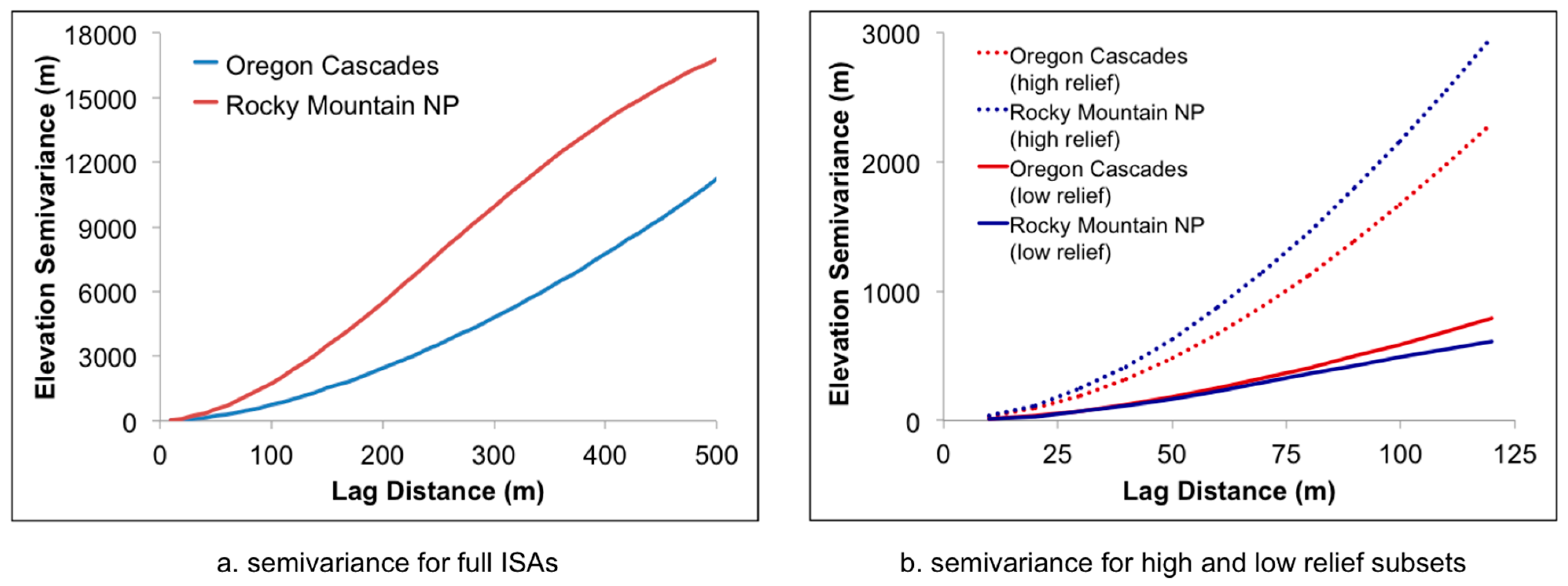
Although the differences between minimum and maximum elevation at each ISA were similar (1033 m for the Oregon Cascades ISA and 829 m for the Rocky Mountain NP ISA), comparison of elevation semivariograms based on 10 m digital elevation data (Figure 3a) indicated higher semi-variance in elevation at the Rocky Mountain NP ISA. In order to allow for comparison between the frequency of occurrence of mixed snow cover pixels at the ISAs that would not be biased by differences in topography, we selected a 1500 × 750 m high-relief subset from each ISA as well as a 1500 × 500 m low-relief subset from each study area (Figure 2). The elevation semivariograms for the high- and low-relief subsets from each study area are shown Figure 3b. For the high- and low-relief subsets at each study area, we repeated the analysis described above for spatial resolutions between 1 m and 125 m. The analysis for the subsets was constrained to 125 m pixels due to the smaller extent of the image subsets.

Figure 3. Semivariograms for elevation derived from 10 m DEM for (a) the Oregon Cascades and Rocky Mountain NP ISAs, and (b) high- and low-relief subsets from the Oregon Cascades and Rocky Mountain NP ISAs.

In order to determine the potential for error in total study area snow cover fraction that might be introduced by monitoring binary SCA rather than fractional SCA at various spatial resolutions, we also calculated total ISA snow cover fraction based on binary SCA at spatial resolutions greater than the original 0.5 m resolution. To accomplish this, at each spatial resolution, r, we first calculated fSCA for each pixel at resolution r using Equation (1) and then calculated the binary SCA-derived study area snow cover fraction, bSCA_r using Equation (3):

{bSCA}_{r} = \frac{\sum_{p = 1}^{p = n} s_{p} {\begin{matrix} s_{p} = 0, f o r f S C A < 0.5 \\ s_{p} = 1, f o r f S C A \geq 0.5 \end{matrix}}{n}

(3)

where n was equal to the total number of pixels at resolution r within the ISA. For this comparison, it was essential that nearly identical samples of high resolution pixels were used for calculations at all spatial resolutions considered. For this reason, we were unable to conduct this analysis at spatial resolutions > 250 m, since the irregularly shaped ISA analysis extent resulted in the elimination of a substantial number of high resolution pixels that fell within the analysis extent but also within an aggregated grid cell that extended beyond the boundary extent.

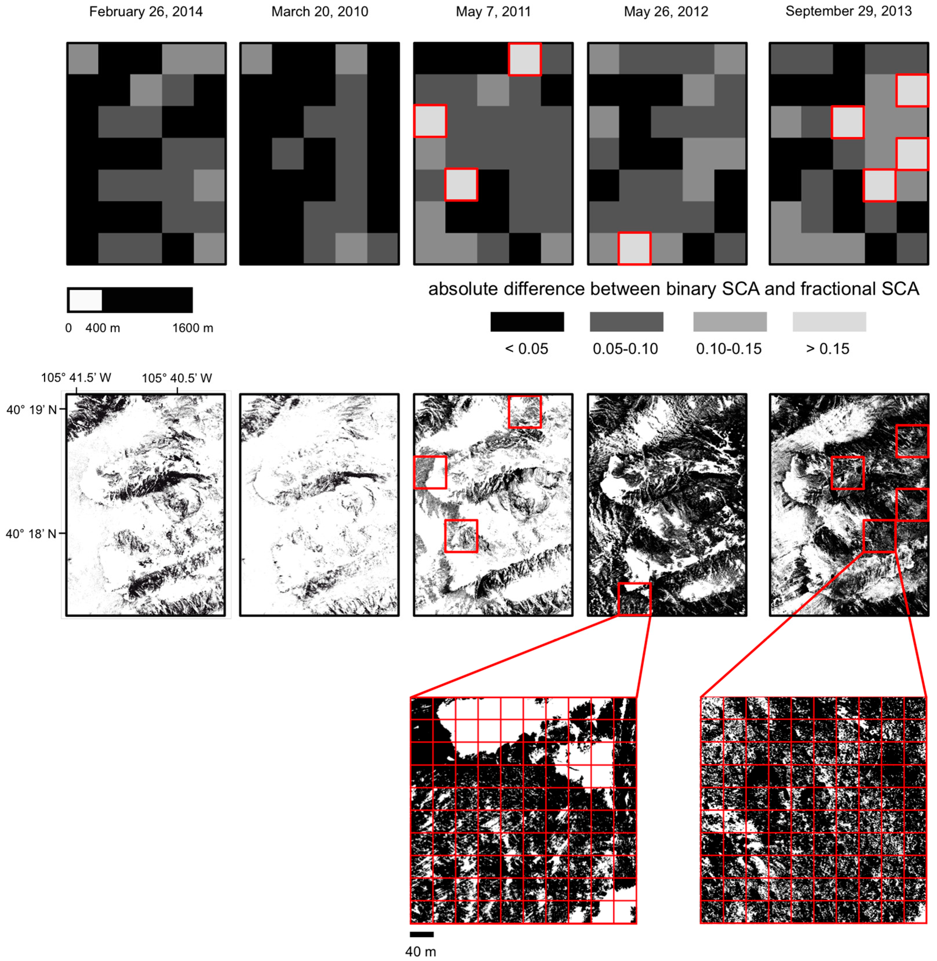
For the Rocky Mountain NP ISA, we conducted additional analysis to determine the overall frequency and spatial distribution of areas where a Landsat scale (~30 m) binary SCA representation characterizing pixels with ≥ 50% snow cover as snow-covered and pixels with < 50% snow cover as snow-free would be prone to error. We chose 40 m spatial resolution for this analysis because, of the pixel resolutions we evaluated (shown in Table 3), the 40 m resolution offered the closest approximation of the estimated ground instantaneous field of view (GIFOV) for the Landsat TM instrument, which is slightly larger than the nominal spatial resolution of 30 m [53]. To map the spatial distribution of potential errors arising from the use of binary SCA, we calculated fSCA using Equation (1) for 40 m pixels, and then calculated bSCA_{40 m} for 400 m blocks corresponding with 10 × 10 arrays of 40 m pixels (rather than for the full ISA extent), using Equation (3). The position of the 10 × 10 (400 m) pixel blocks was determined by the ISA boundary, with the origin point for the grid located at the northwestern corner of the image. We then calculated fSCA for each 400 × 400 m block using the original 0.5 m resolution binary image and the approach described in Equation 1 and compared fSCA to bSCA_40m at each block, calculating the mean absolute difference between fSCA and bSCA_40m. By comparing fSCA and bSCA_40m at each block, we calculated the error that would be expected to occur for blocks of 100 40 m pixels if 40 m binary, rather than 40 m fractional SCA, was used. It is important to note that we were estimating differences that might arise from binary vs. fraction SCA mapping at 40 m spatial resolution, and in this case, 400 m was the size of the aggregation unit that corresponded to a 10 × 10 array of 40 m pixels, but not the spatial resolution of interest.

2.6. In Situ Snow Cover Monitoring Overview

In order to estimate the prevalence of partially snow-covered conditions for individual grid cells similar in size to Landsat pixels, we conducted in situ fractional SCA monitoring at 60 m grid cells at two field study areas in the Rocky Mountains of Colorado (Figure 1) between September 2013 and August 2014. In situ fractional SCA data collected at these footprints will be used as part of an ongoing effort for validation of a Landsat fractional SCA product currently under development, and consequently we opted for monitoring 60 m footprints rather than 30 m footprints (the nominal pixel size for Landsat). The 60 m footprint size was selected because the effective resolution of Landsat has been shown to be larger than the 30 m nominal resolution [53], and also because monitoring the larger 60 m footprint would reduce the impact of spatial registration errors on comparisons between in situ and remotely sensed data.

2.7. In Situ Snow Cover Monitoring Study Sites

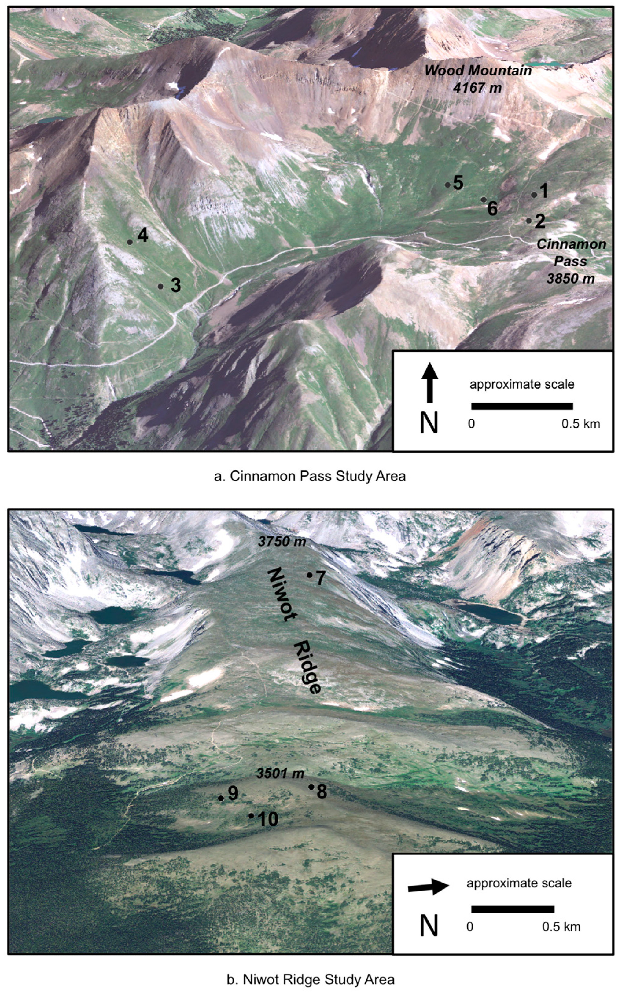
At the first FSA, referred to from this point forward as the Cinnamon Pass FSA, we measured daily snow cover fraction over six 60 × 60 m footprints in the vicinity of Cinnamon Pass in the San Juan range of the Colorado Rocky Mountains (Figure 4a). Sites ranged in elevation from 3669 to 3864 m, with slope angles ranging from 11° to 28° (Table 3). Modeled mean annual precipitation at the study area for the period 1981–2010 computed from the PRISM climate dataset [46] ranged from 1169 to 1320 mm; mean January temperatures ranged from −9.7 °C to −8.6 °C and mean July temperatures ranged from 8.4 °C to 10.0° C for the same period.

Figure 4. Locations for 60 × 60 m grid cells instrumented with arrays of temperature data loggers at (a) the Cinnamon Pass FSA and (b) the Niwot Ridge FSA.

At the second FSA, referred to from this point forward as the Niwot Ridge FSA, we measured daily snow cover fraction at four 60 × 60 m footprints at and above the alpine tree line on Niwot Ridge (Figure 4b), located about 3 km east of the continental divide in the Rocky Mountains west of Boulder, Colorado. Footprints at the Niwot Ridge FSA ranged in elevation from 3425 to 3666 m and included slope angles from 10°–19° (Table 4). While two of the four sites were > 200 m above tree line and included only herbaceous and dwarf shrub vegetation, two sites were within 20 m of stunted spruce and fir trees, which could be found throughout the area above the upper limit of contiguous upright forest. Modeled mean annual precipitation at the study area for the period 1981–2010 computed from the PRISM climate dataset ranged from 1017 to 1068 mm, with mean January temperatures ranging from −10.7 °C to −9.4 °C and mean July temperatures ranging from 9.3 °C to 11.1 °C for the same period (Table 3).

Table 4. Study area location and site characteristics for 60 × 60 m grid cell footprints where in situ monitoring was conducted. CP indicates Cinnamon Pass, while NR indicates Niwot Ridge.

**Table 4.** Study area location and site characteristics for 60 × 60 m grid cell footprints where in situ monitoring was conducted. CP indicates Cinnamon Pass, while NR indicates Niwot Ridge.
Site	Field Study Area	Elevation (m)	Slope (Degrees)	Aspect	Land Cover	Local Topographic Position
1	CP	3850	11	W	rocky alpine meadow	ridgetop
2	CP	3845	15	NW	rocky alpine meadow	ridgetop
3	CP	3669	28	SE	alpine meadow	mid-slope
4	CP	3784	27	E	alpine meadow	mid-slope
5	CP	3779	15	S	alpine meadow	mid-slope
6	CP	3776	12	NW	alpine meadow	valley
7	NR	3666	19	N	rocky alpine meadow	near ridgetop
8	NR	3496	10	N	rocky alpine meadow	ridgetop
9	NR	3425	19	S	talus slope	mid-slope
10	NR	3430	14	S	rocky alpine meadow	valley

2.8. In Situ Snow Cover Monitoring Approach

At each of 10 monitoring sites within our field study areas, we buried 16 HOBO Pendant temperature data loggers 2–5 cm below the soil surface (Mention of a particular product does not constitute endorsement by the U.S. federal government). At one site where the pixel footprint was dominated by a rocky talus slope, some data loggers were placed below rocks near the surface of the talus pile. Our placement of data loggers varied from the approach used by Raleigh et al. [54] in the spatial resolution of the footprint monitored (60 × 60 m in our study vs. 500 × 500 m in Raleigh et al. [54]), the number of sensors deployed, and the placement of sensors within the footprint. While Raleigh et al. 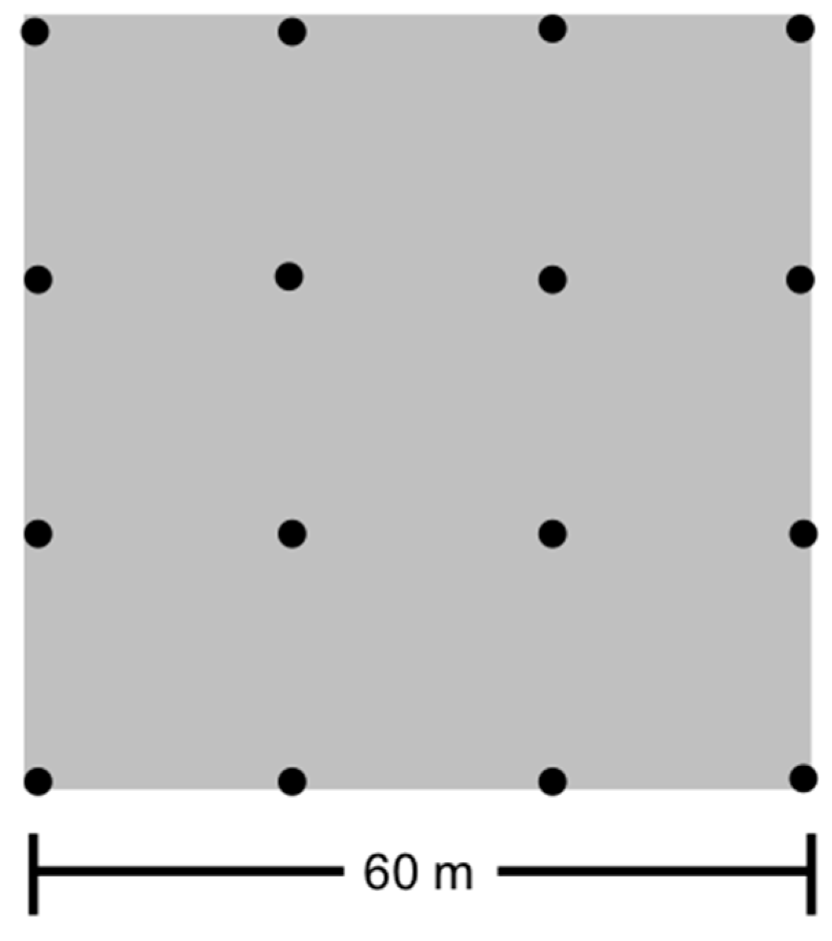[54] deployed between 37 and 89 sensors in several different sensor configurations, including quasi-regular grids and transects, all of which covered 500 × 500 m or larger areas, we used regular 4 × 4 grids with 20 m spacing at each site, for a total of 16 sensors covering each 60 × 60 m footprint (Figure 5).

Figure 5. Schematic diagram of the arrangement of temperature data loggers at each 60 × 60 m grid cell footprint. Data loggers are indicated by black circles.

Each data logger recorded the temperature at 1.5-hourly intervals. At the Cinnamon Pass study area, loggers were installed in mid-September 2013 and collected in July–August 2014, while at the Niwot Ridge study area loggers were installed in mid-October 2013 and also collected in July–August 2014. While 16 temperature data loggers were installed at each site, in a few cases, we were unable to locate a buried temperature data logger, and in a few other cases, data loggers stopped recording due to malfunction or insufficient battery voltage. All data from temperature data loggers that stopped recording prior to retrieval were discarded in order to ensure that calculated snow cover fraction would be based on the same set of points for the entire monitoring period.

We used the algorithm introduced by Raleigh et al. [54] to convert the 1.5-hourly temperature time series from individual sensors to a daily snow cover fraction value for each 60 m grid cell footprint. Snow cover located above a sensor insulates the uppermost layer of the soil, resulting in a substantial reduction of the range in temperature variability experienced near the soil surface [7]. At temperate sites, in the absence of snow cover there is typically a strong diurnal ground temperature oscillation that disappears when snow cover is present. Monitoring this daily ground temperature variation allows for the identification of periods of snow cover using time series data collected at hourly to several hour increments [54,55,56,57]. Automated classification of periods with snow cover requires the selection of an appropriate 24-hour temperature range threshold; 24-hour periods where the temperature range is below this value will be classified as snow-covered. No single value has been established in the literature as appropriate for all conditions, as ground surface temperature variability is affected by a number of factors, including soil type, soil moisture, depth of burial, air temperature variability, and incoming solar radiation. We selected a 24-hour temperature range threshold of 2 °C, considerably larger than the temperature threshold used by Raleigh et al. and other studies [54,55,56,57]. Visual interpretation of temperature time series data suggested that this higher value allowed for identification of shallow snow cover during mid-winter while having minimal impact on the classification of snow cover conditions during the spring and summer melt period.

For each sensor that recorded data for the entire monitoring period, for each interval in the 1.5-hourly time series we calculated the difference between minimum and maximum temperatures recorded for the previous 24 h as well as the next 24 h in the time series. If the 24-hour temperature range value exceeded 2 °C for either the previous 24-hour period or the upcoming 24-hour period, the 1.5-hourly time series snow cover value was set to 0, indicating snow-free conditions. If the 24-hour temperature range values for both periods were less than 2 °C, the 1.5-hourly time series snow cover value was set to 1, indicating snow-covered conditions. Snow cover fraction on the ground at time series interval t, fSCA_t was then calculated for each interval in the time series using Equation (4):

{fSCA}_{t} = \frac{\sum_{l = 1}^{l = n} s_{l}}{n}

(4)

where s_l was binary snow presence, indicated by 1, or absence, indicated by 0, at temperature data logger l. We then computed the mean daily snow cover fraction for the footprint, fSCA_d, using Equation (5):

{fSCA}_{d} = \frac{\sum_{t = 1}^{t = 16} {fSCA}_{t}}{16}

(5)

While we were not able to validate the methodology for monitoring grid cell snow cover fraction at any of the 60 m footprints in this study, photographic survey data collected at five 60 m footprints at high-elevation subalpine forest and meadow sites in Utah and California indicated good agreement between photo-derived snow cover fraction and snow cover fraction calculated from similar grids of temperature data loggers using the same approach (mean absolute difference 0.09) [58].

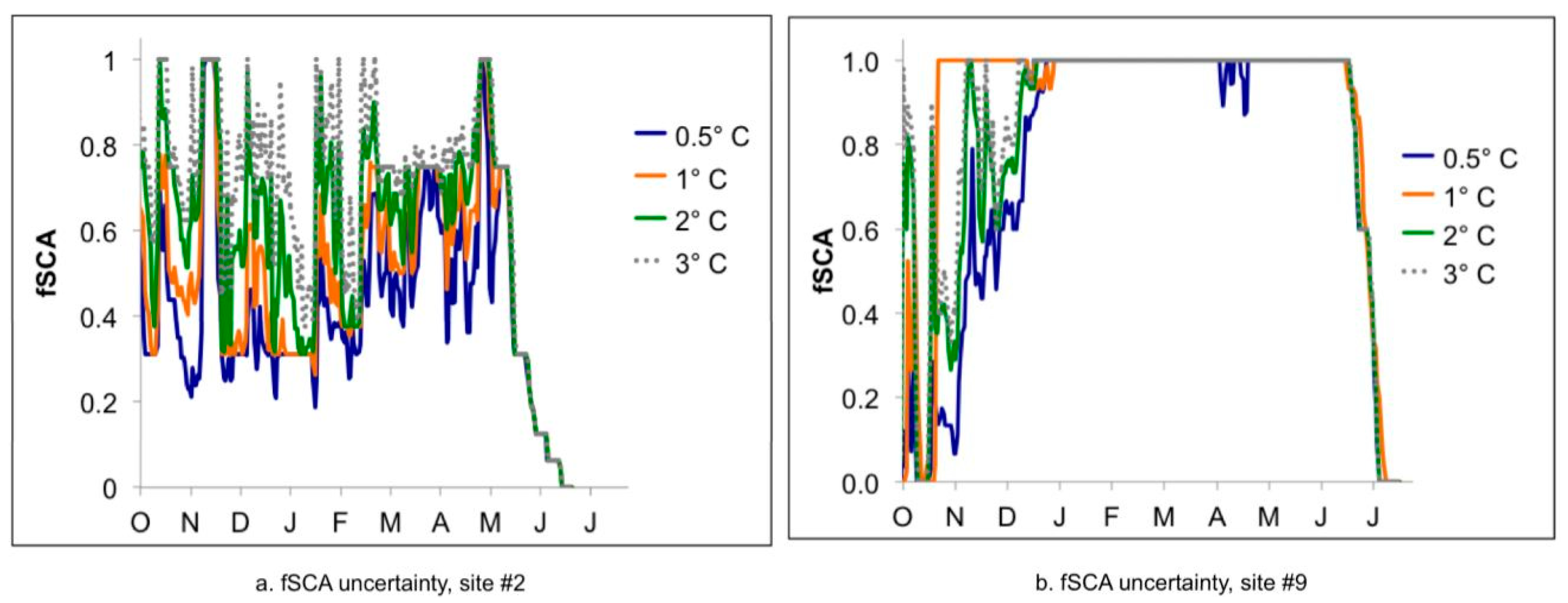
In order to gauge the impact of the 24-hour temperature range value threshold on computed snow cover fraction, we conducted a sensitivity analysis where we computed the daily snow cover fraction using values of 0.5 °C, 1 °C, 2 °C and 3 °C. For each day in the time series, we calculated uncertainty in grid cell snow cover fraction, fSCA_u, by calculating the difference between snow cover fraction computed using the 0.5 °C threshold, fSCA_0.5, and snow cover fraction computed using the 3 °C threshold, fSCA_3.0, using Equation (6):

{fSCA}_{u} = {fSCA}_{3.0} - {fSCA}_{0.5}

(6)

fSCA_u had a theoretical range from 0 (indicating no difference between snow cover fraction computed using a 0.5° C threshold and snow cover fraction computed using a 3 °C threshold) to 1 (indicating no snow cover computed using a 0.5 °C threshold and full snow cover computed using a 3 °C threshold).

3. Results

3.1. High Spatial Resolution Binary Snow-Covered Area

Binary SCA classifications at 0.5 m spatial resolution for the Oregon Cascades and Rocky Mountain NP ISAs are shown in Figure 6 and Figure 7, with examples from each study area shown in Figure 8. Total study area snow cover fraction for each date from the two ISAs ranged from 0.143 to 0.943 (Table 2). Classification accuracy for the 0.5 m binary SCA classifications ranged from 81%–98%, with a mean of 90% for all 10 images (Table 2). Mean classification accuracy was slightly higher at the Oregon Cascades ISA (92.0%) than at the Rocky Mountain NP ISA (87.4%). Mean classification accuracy was very similar for the three dates where pan-sharpened three-band imagery was used (89.9%) and the three dates where panchromatic imagery was used (89.3%)

3.2. Prevalence of Mixed Pixels across Spatial Resolutions and between Study Areas

The fraction of mixed pixels at spatial resolutions between 1 m and 500 m is shown in Figure 9. At 40 m spatial resolution, slightly larger than the estimated GIFOV for Landsat at nadir, mixed pixels accounted for 25%–50% of total pixels at the Oregon Cascades ISA (mean of 36% for five dates), and 41%–93% of total pixels at the Rocky Mountain NP ISA (mean of 69% for five dates). At 500 m, the nominal spatial resolution for MODIS, mixed pixels accounted for 67%–93% of total pixels at the Oregon Cascades ISA (mean of 81% for five dates) and from 79%–100% of total pixels at the Rocky Mountain National Park ISA (mean of 93% for five dates). While the fraction of mixed pixels varied substantially across the available imagery dates for each ISA, the fraction of mixed pixels was consistently higher at the Rocky Mountain NP ISA than at the Oregon Cascades ISA.

Figure 6. WorldView imagery (top row) and high-resolution binary snow-covered area maps (bottom row) for the Oregon Cascades ISA. Panchromatic band data is displayed for the 15 July 2011 and 29 November 2013 images, while red band data is displayed for the 12 May 2011, 1 September 2013, and 26 December 2013 images.

Figure 7. WorldView imagery (top row) and high-resolution binary snow-covered area maps (bottom row) for the Rocky Mountain NP ISA. Panchromatic band data is displayed for 7 May, while red band data is displayed for the 26 February 2014, 20 March 2010, 26 May 2012, and 29 September 2013 images.

Figure 8. Examples of 0.5 m binary snow-covered area classifications (right side) based on WorldView 2 imagery (left side). Oregon Cascades, 26 December 2013, (panels a and b) and Colorado Rocky Mountains, 26 February 2014 (panels c and d).

Figure 9. Fraction of mixed (partially snow-covered) pixels for pixel resolutions between 1 m and 500 m, for (a) the Oregon Cascades imagery study area, and (b) the Rocky Mountain NP imagery study area. Vertical blue lines indicate 40 m spatial resolution (slightly above the nominal spatial resolution for Landsat) and 500 m spatial resolution (the nominal spatial resolution for MODIS).

The high-relief subset from the Oregon Cascades ISA and the corresponding high-relief subset from the Rocky Mountain NP ISA exhibit similar semivariograms, while the low-relief subsets from the two study areas exhibit nearly identical semivariograms (Figure 3b). Comparisons of the fraction of mixed pixels at spatial resolutions between 1 m and 125 m indicate higher prevalence of mixed pixels at the Rocky Mountain NP ISA in both the high-relief and low-relief subsets (Figure 10).

Figure 10. (a) Fraction of mixed pixels for Oregon Cascades ISA high-relief subset, (b) fraction of mixed pixels for the Rocky Mountain NP ISA high-relief subset, (c) fraction of mixed pixels for the Oregon Cascades ISA low-relief subset, and (d) fraction of mixed pixels for the Rocky Mountain NP ISA low-relief subset. Vertical blue lines indicate 40 m, slightly above the nominal spatial resolution of Landsat.

3.3. Differences between Binary and Fractional SCA

Our analysis indicated that as spatial resolution became coarser, the difference between study area snow cover fraction computed from binary SCA and fractional SCA, and thus the potential for error in binary SCA mapping, tended to increase (Figure 11). In general, if the 0.5 m snow cover fraction was > 0.6, binary snow cover fraction for the study area tended to increase at coarser spatial resolutions, while if the 0.5 m snow cover fraction was < 0.6, binary snow cover fraction for the study area tended to decrease at coarser spatial resolutions. While differences between study area snow cover fractions derived from binary versus fractional SCA were generally small, the change in study area snow cover fraction with spatial resolution was more significant for the July 2011 image from the Oregon Cascades ISA, with the study area snow cover fraction increasing from 0.67 at 0.5 m to 0.85 at 250 m.

Figure 11. Relationship between pixel resolution and total study area snow cover fraction derived from binary SCA for (a) Oregon Cascades ISA (b) and Rocky Mountain NP imagery ISA. Vertical blue lines indicate 40 m, slightly above the nominal spatial resolution of Landsat.

Figure 12. Spatial distribution of 400 × 400 m blocks from the Rocky Mountain NP imagery study area where absolute differences between binary and fractional SCA were low (< 0.05), medium (0.05–0.10), high (0.10–0.15), and highest (> 0.15).

More detailed analysis of the spatial and temporal distribution of the differences between binary and fractional SCA at 40 m spatial resolution were conducted for the Rocky Mountain NP ISA. For a grid of 400 × 400 m blocks, we mapped the absolute difference between block snow cover fraction derived from 40 m binary SCA and block snow cover fraction derived from the original 0.5 m binary SCA image. Although the majority of 400 m blocks indicated absolute differences between binary and fractional SCA < 0.10, a number of blocks with absolute differences between binary and fractional SCA > 0.15 were identified at the Rocky Mountain National Park ISA (Figure 12). Snow cover within each of these blocks exhibited very fine scale variability in the original 0.5 m snow cover image.

3.4. Prevalence of Partially Snow-Covered Conditions at In Situ Monitoring Sites

In contrast to the results of the imagery analysis, which allowed us to calculate the prevalence of partially snow-covered pixels over a range of scales for many pixels on just a few dates, the in situ snow cover fraction measurements allowed us to calculate the prevalence of partial snow cover conditions at ten 60 m pixel footprints over all days for a 10-month period. Summary fractional SCA statistics computed from temperature data loggers are presented in Table 5. As mentioned previously, in a few cases, we were unable to locate a buried temperature data logger, and in a few other cases, data loggers malfunctioned or stopped recording due to insufficient battery voltage. The total number of temperature data loggers used for calculation of snow cover fraction varied between 12 and 16, with valid data available from at least 14 sensors for eight of the 10 sites (Table 5).

Daily time series of snow cover fraction for five of the six grid cells monitored at the Cinnamon Pass FSA and three of the four grid cells monitored at Niwot Ridge FSA are shown in Figure 13. Daily grid cell snow cover fraction calculated from temperature data logger arrays indicate that snow cover conditions at grid cell footprints fell into two distinct categories. At four of the 10 sites, full snow cover across the grid cell footprint occurred only rarely (3–45 days), despite snow covering a portion of the footprint for as many as 243 days during the monitoring period. At the remaining six sites, the grid cell footprint was fully snow covered between February 1 and late spring or early summer, with partial snow cover conditions common for some footprints during the earlier part of the season. For the six footprints with continuous or near continuous full winter snow cover, the first day with less than full snow cover after 1 April occurred between 3 May and 5 July. The length of the transition period between fully snow-covered and fully snow-free conditions ranged from 17–56 days, while the mean transition period length was 37 days.

Table 5. Full, partial, and total snow cover days, as well as snow-covered to snow-free transition period metrics for 60 × 60 m footprints. Transition period metrics were not calculated for sites with intermittent winter snow cover. CP indicates Cinnamon Pass, while NR indicates Niwot Ridge. fSCA indicates fractional snow-covered area.

**Table 5.** Full, partial, and total snow cover days, as well as snow-covered to snow-free transition period metrics for 60 × 60 m footprints. Transition period metrics were not calculated for sites with intermittent winter snow cover. CP indicates Cinnamon Pass, while NR indicates Niwot Ridge. fSCA indicates fractional snow-covered area.
Site	Study Area	Valid Sensors	Snow Cover Days			Partial/Total Ratio	First Day
Site	Study Area	Valid Sensors	Full	Partial	Total	Partial/Total Ratio	< 1.0 fSCA	< 0.5 fSCA	Snow-Free	Length (days)
1	CP	14	17	223	240	0.93	-	-	-	-
2	CP	16	16	243	259	0.94	-	-	-	-
3	CP	15	144	99	243	0.41	3 May	21 May	15 June	43
4	CP	16	235	25	260	0.10	9 June	23 June	2 July	23
5	CP	16	229	39	268	0.15	1 June	16 June	10 July	39
6	CP	16	242	61	303	0.20	18June	7 July	13 Aug.	56
7	NR	15	45	223	268	0.83	-	-	-	-
8	NR	12	3	183	186	0.98	-	-	-	-
9	NR	15	186	88	274	0.32	5 July	17 July	22 July	17
10	NR	13	162	137	299	0.46	29 June	15 July	13Aug.	45

Figure 13. Daily 60 m grid cell snow cover fraction time series from (a) grid cells 1, 5, and 6 at Cinnamon Pass FSA (b), grid cells 3 and 4 at Cinnamon Pass FSA, and (c) grid cells 8, 9, and 10 at Niwot Ridge FSA. Time series depicted in the same panel are all from grid cells within 500 m and could thus be contained within a single 500 m MODIS grid cell. Time series from the two 60 m grid cells not shown are similar to #1 (south facing) in panel (a) and #8 (ridgetop) in panel (c).

3.5. Sensitivity of Calculated Snow Cover Fraction to 24-Hour Temperature Range Threshold

Results from the sensitivity analysis of the effect of 24-hour temperature range threshold on calculated snow cover fraction at each footprint indicate that, at sites where partially snow-covered conditions were common throughout the winter, calculated snow cover fraction was highly sensitive to the temperature threshold value used in the algorithm (Figure 14a, Table 6). At sites where fully snow-covered conditions persisted throughout the winter, calculated snow cover fraction was much less affected by varying the temperature threshold (Figure 14b, Table 6). The mean grid cell snow cover fraction uncertainty (in terms of snow cover fraction, ranging from 0–1) for all days between 15 October and the last day with snow cover ranged from 0.01 to 0.39 (Table 6), with an overall mean of 0.16 for all sites and all days. When only the period between 1 April and the last day of snow cover was considered, mean uncertainty was lower at all sites, ranging from 0 to 0.24, with an overall mean of 0.08. For the 15 October—snow-free period, the fraction of days with uncertainty in snow cover fraction > 0.1 ranged from < 0.01–0.86, while for the 1 April—snow-free period, the fraction of days with uncertainty in snow cover fraction > 0.1 ranged from 0–0.67. During the 1 April—snow-free period, the fraction of days with > 0.1 uncertainty at five of the 10 sites was ≤ 0.03.

Figure 14. Results from sensitivity analysis indicating 60 m grid cell snow cover fraction using 0.5 °C, 1 °C, 2 °C, and 3 °C temperature thresholds for (a) an example site with partially snow-covered conditions throughout the winter and spring (site #2) and (b) for an example site with consistent fully snow-covered conditions throughout the winter and spring (site #9).

Table 6. Snow cover fraction uncertainty metrics for each 60 m grid cell. Uncertainty is expressed in terms of snow cover fraction ranging from 0 to 1.

**Table 6.** Snow cover fraction uncertainty metrics for each 60 m grid cell. Uncertainty is expressed in terms of snow cover fraction ranging from 0 to 1.
Site	Valid Sensors	Partial/Total Snow Cover Days Ratio	15 October—Snow-Free Date			1 April—Snow-Free Date
Site	Valid Sensors	Partial/Total Snow Cover Days Ratio	Total Days	Mean Uncertainty	Fraction of Days with Uncertainty > 0.10	Total Days	Mean Uncertainty	Fraction of Days with Uncertainty > 0.10
1	14	0.93	240	0.29	0.86	72	0.22	0.67
2	16	0.94	258	0.26	0.76	91	0.13	0.45
3	15	0.41	241	0.11	0.35	75	0.02	0.00
4	16	0.10	257	0.01	0.00	92	0.00	0.00
5	16	0.15	264	0.04	0.12	100	0.03	0.13
6	16	0.20	297	0.03	0.13	135	0.02	0.00
7	15	0.83	262	0.39	0.81	100	0.16	0.49
8	12	0.98	216	0.29	0.81	55	0.24	0.69
9	15	0.32	272	0.09	0.26	112	0.01	0.03
10	13	0.46	293	0.12	0.29	134	0.01	0.01
Mean:	-	-	-	0.16	0.44		0.08	0.25

4. Discussion

Our analysis of mixed pixel prevalence across spatial resolutions indicates that mixed pixels occur frequently across the alpine landscape even at fine spatial resolutions (< 10 m), and that they often dominate the landscape at the spatial resolution imaged by Landsat (nominally 30, with true GIFOV closer to 40 m). For our analysis, we defined mixed pixels as pixels with fSCA between 0.02 and 0.98. While these thresholds may seem quite lax for identification of mixed pixels (or conversely, quite strict for identification of pure pixels), our goal was to estimate the fraction of the alpine landscape at different places, times, and spatial resolutions where sub-pixel variability in snow-covered area was present. The thresholds of 0.02 and 0.98 were chosen in lieu of 0 and 1 to account for occasional noise in the data. Our definition of mixed pixels will likely result in identification of more mixed pixels than would be mapped using Landsat and MODIS, since fSCA mapping algorithms such as MODSCAG often have difficulty mapping snow cover at fractions < approximately 0.15, while Landsat-based algorithms will be prone to overestimation of snow cover when saturation of the visible bands occurs, resulting in fewer mixed pixels when snow cover fractions are slightly below 1. Nevertheless, we believe it is important to quantify the prevalence of all mixed snow cover pixels, including those where the fraction of snow-covered or snow-free ground is quite small. Even very small differences in pixel fSCA, such as the difference between fSCA fractions of 1.0 and 0.97 can potentially indicate substantial differences in snow cover conditions, such as the difference between end of winter conditions with deep snow cover and conditions later in the spring where snow water equivalent has been reduced by 50% but only a tiny fraction of the pixel has melted out.

We found that mixed pixels were more common across all spatial scales and dates at our continental ISA in Colorado than at our maritime ISA in Oregon. It is possible that the more rugged topography at the Rocky Mountain NP ISA may be partially responsible for this difference. The increased prevalence of mixed pixels across all dates can still be observed, however, even when subsets with similar topographic characteristics are compared, at least for spatial resolutions < 125 m.

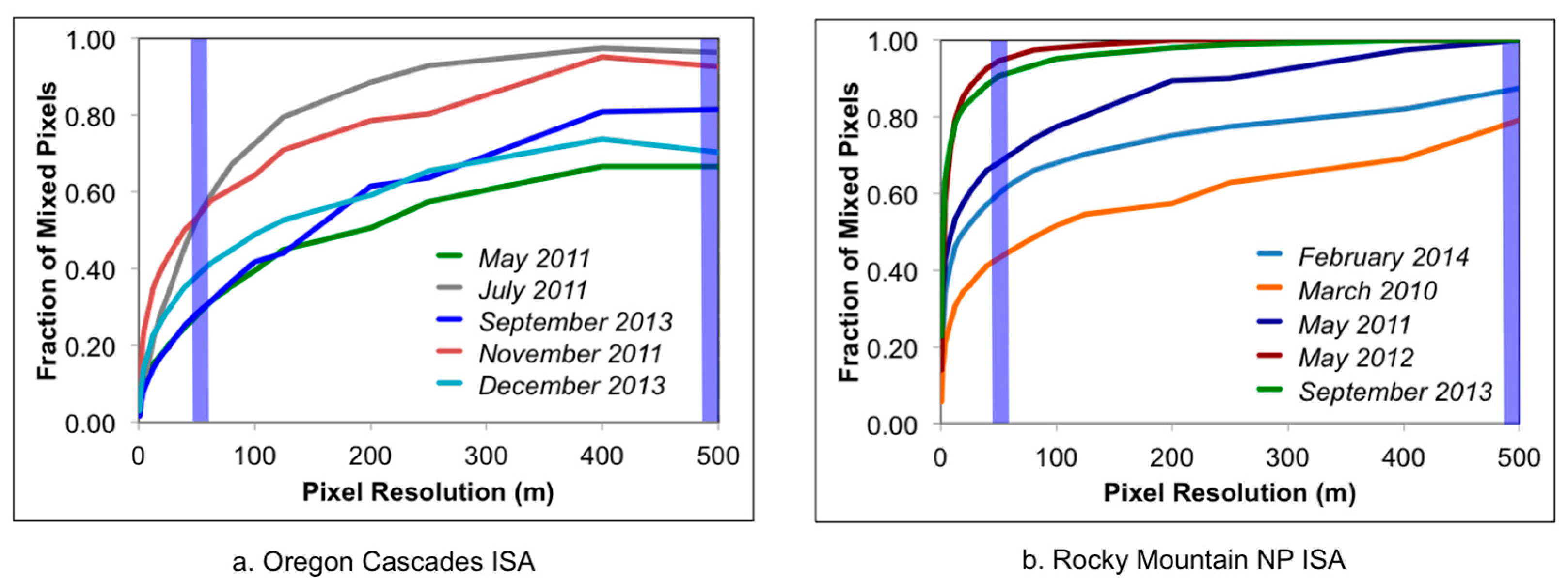
Differences between recent snowfall histories at the two ISAs prior to image acquisition are also insufficient to explain the greater prevalence of mixed pixels at the Rocky Mountain NP ISA, although heavy snow accumulation prior to the date of image acquisition did appear to reduce the incidence of mixed pixels in the Rocky Mountain NP ISA relative to other dates without recent heavy snow accumulation at the same ISA. At the Rocky Mountain NP ISA, the prevalence of mixed pixels was much lower for the three dates with ≥ 16 mm snow water equivalent accumulation over the previous 10 days (26 February 2014, 20 March 2010, and 7 May 2011) than for the two dates with little or no new snow over the previous 10 days (26 May 2012 and 29 September 2013) (Figure 9b). Heavy snow accumulation did not appear to have as pronounced an effect on the prevalence of mixed pixels in the Oregon Cascades ISA (Figure 9).

If differences in recent snow accumulation were the primary factor responsible for differences in the prevalence of mixed pixels between the two ISAs, we would expect to find a higher incidence of mixed pixels at the Oregon Cascades ISA than at the Rocky Mountain NP ISA, since no snowfall occurred within 10 days for three of the five dates analyzed at the Oregon Cascades ISA. Instead, we found the incidence of mixed pixels at the Oregon Cascades ISA was actually consistently lower than the incidence of mixed pixels at the Rocky Mountain NP ISA. We hypothesize that, over the course of the winter, the combined effects of lower moisture content during snow accumulation events, lower overall precipitation, and higher wind speeds (Table 1) resulted in the development of a more heterogeneous snow cover at the continental Rocky Mountain NP ISA than at the Oregon Cascades ISA. Snowfall events with high moisture content (a common occurrence in the maritime snow climate of the Oregon Cascades) are more likely to coat all terrain surfaces evenly during accumulation. In contrast, snowfall events with lower moisture content (a common occurrence in the Colorado Rockies) often result in less uniform accumulation, a situation that is exacerbated by consistently higher wind speeds.

Finally, it is also possible that differences in very fine scale surface roughness that cannot be captured by a 10-m DEM may also play a role in explaining the differences between the prevalence of mixed pixels at these two study areas.

It is worth noting that a significant but unknown fraction of the snow cover mapped in the 1 September 2013 image from the Oregon Cascades ISA consisted of exposed glacial ice as well as snow cover from the current year on top of glacial ice, particularly within the high-relief subset image (Figure 2). While the presence of glacier cover raises the overall ISA snow cover fraction, it is also likely to reduce the prevalence of mixed pixels at the spatial resolutions considered here, since glaciers represent a large mass of contiguous ice and snow that might otherwise be occupied by a patchy distribution of late-lying seasonal snow cover patches.

The observation that portions of the alpine landscape remain free of snow cover across much of the winter and spring while other areas remain snow covered well into the summer is not novel. The daily 60 m snow cover fraction time series computed from 1.5-hourly temperature data collected near the ground surface, however, allowed us to quantify the frequency of partially snow-covered conditions at a scale similar to that provided by Landsat. While the calculated snow cover fraction for pixel footprints with intermittent snow cover appeared to be quite sensitive to the 24-hour temperature range threshold used to classify the presence or absence of snow cover above each sensor, the results from the uncertainty analysis still indicated that, regardless of the temperature range threshold value used, partial snow cover conditions occurred with great frequency throughout the winter and spring. For the remaining sites, where snow covered the entire pixel footprint for most or all days prior to the spring snowmelt period, the temperature range threshold value appeared to matter very little, suggesting that snow cover fraction estimates for these footprints can be considered more reliable.

At the four sites where partially snow-covered conditions were common throughout the winter and spring, monitoring per-pixel snow cover fraction provides a clear advantage over binary monitoring approaches that use an arbitrary, potentially variable fractional snow cover threshold to classify a pixel as snow-covered or snow-free. At this type of site, binary snow cover classifications will consistently overestimate the true snow cover fraction for most instances when snow covers > 50% of the pixel footprint and consistently underestimate the true snow cover fraction for most instances when snow covers < 50% of the land surface, although aggregation of results from many pixels can reduce the magnitude of the error. While at first glance, the need for a fractional monitoring approach may seem less obvious for sites where fully snow-covered conditions occur throughout the winter, the spring transition period between fully snow-covered and fully snow-free conditions at these sites spanned a period when 2–4 scenes would be collected by a single Landsat instrument (with the potential for even more scenes during periods of concurrent Landsat missions and in areas covered by more than one orbital path). During this transition period, there is an obvious benefit to retrieving per-pixel snow cover fraction, rather than simply the presence or absence of snow cover, as per-pixel fractional snow-covered area can provide detailed information on the progression of snowmelt at the pixel rather than just a vague approximation of the time when the pixel transitioned from > 50% snow cover to < 50% snow cover.

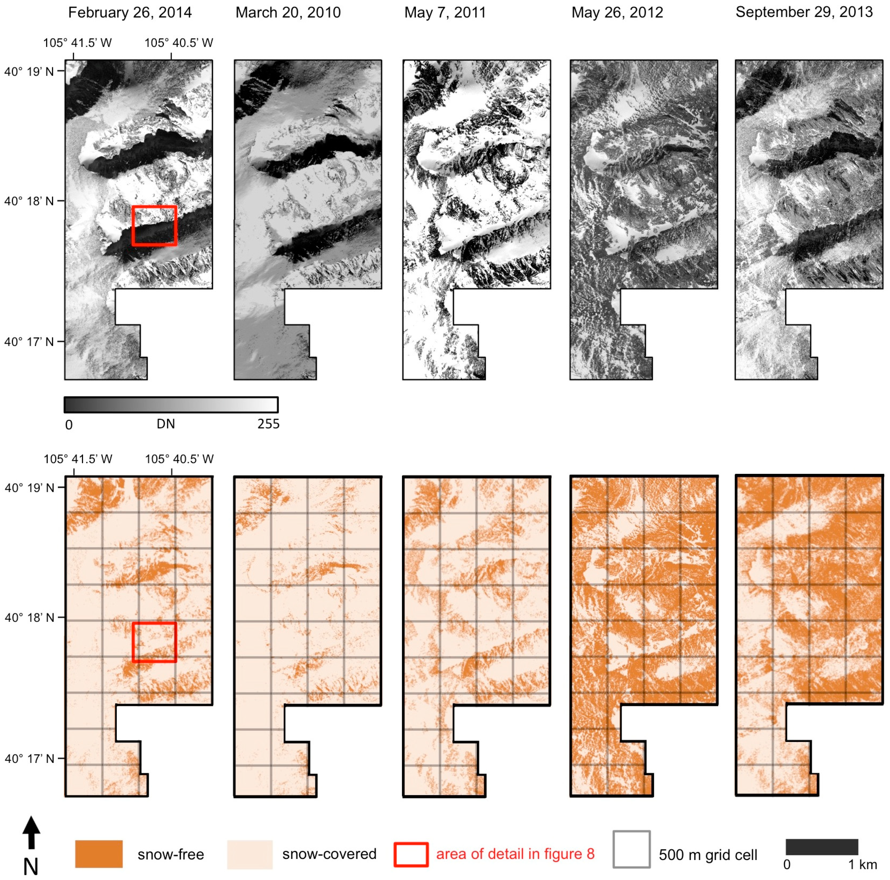
The rarity of pure pixels at 500 m spatial resolution and the sometimes dramatic differences in snow cover conditions that often exist in close proximity within 500 m grid cells (as demonstrated in Figure 13) present a strong case for the necessity of adopting a fractional SCA mapping approach when working with MODIS data in high mountain areas. It is important to note that for an instrument such as MODIS, the actual ground instantaneous field of view (GIFOV) represented by a single pixel is always larger than the nominal spatial resolution of 500 m, as only approximately 75% of the signal originates from within the nominal 500 m field of view [59]. In addition, for pixels imaged near the edge of the scan, where the scan angle can be as high as 55°, the GIFOV represented in a single pixel is approximately 10× as large as at nadir [60]. While this study does not directly address the frequency of mixed pixels for ground instantaneous fields of view larger than 500 × 500 m, for resolutions between 1 m and 500 m, the probability of mixed pixels generally continues to increase with increasing pixel size, and thus it seems likely that mixed pixels would occur even more frequently for cases where the GIFOV is substantially larger, as it is for MODIS pixels not located near the center of the scan. Ultimately, the vast diversity of conditions within a single MODIS pixel footprint, even at the nominal 500 m spatial resolution, emphasizes the utility of finer scale remote sensing using Landsat or a similar finer resolution platform.

The lower incidence of mixed pixels at the Landsat spatial resolution suggests that a binary SCA mapping approach may be acceptable for some applications in mountain regions at the Landsat scale. For example, in a larger basin with a diversity of slopes and aspects, binary SCA overestimation of snow cover on north-facing slopes with 75% snow cover may often be offset by underestimation of snow cover on south-facing slopes with 25% snow cover, resulting in a basin-wide SCA estimate that closely approximates the true SCA for the basin. However, for basins with more homogeneous terrain at scales > 30 m, monitoring of individual slopes, and any applications where highly accurate spatial distributions are essential, the additional information provided by a fractional SCA dataset provides a major advantage.

For many applications, the most important measure of snowpack is the snow water equivalent (SWE) or snow depth. While optical remote sensing cannot be used directly for monitoring either SWE or snow depth, there is a strong link between SWE and SCA [61], and SCA retrievals from optical sensors can be used in a variety of ways to assist with the estimation of snow depth or SWE. These include the provision of melt-out dates used for SWE reconstruction [1,2,3], constraining modeled SWE to areas where snow cover is actually present [4], and providing the spatial distribution of snow cover for validation of modeled snow cover evolution over space and time [62,63]. In all of these cases, there is a benefit to using fractional SCA at 30 m spatial resolution, particularly if the modeling occurs at 30 m spatial resolution or finer.

It is important to note that the above discussion assumes similar accuracy in retrievals of both binary and fractional SCA. Highly accurate binary SCA data will always remain more useful than fractional SCA data of poor quality. Likewise, highly accurate fractional SCA data will always be more useful than poorer quality binary SCA data.

5. Conclusions

While mixed snow-covered/snow-free pixels can occur at any spatial resolution, at both of our ISAs, mixed pixels become increasingly common at coarser spatial resolutions. The curves representing the fraction of mixed pixels versus spatial resolution varied substantially depending on total study area snow cover fraction, time of year, and snow climate regime. Mixed pixels were more prevalent at the colder, drier continental study area. At the Landsat spatial resolution, mixed pixels comprised 36% of the total pixels over all dates in the Oregon Cascades ISA and 69% of the total pixels for the Rocky Mountain NP ISA. At the MODIS spatial resolution, mixed pixels comprised 81% of the total pixels over all dates in the Oregon Cascades and 93% of the total pixels for the Rocky Mountain NP ISA.

Daily fractional SCA calculated from in situ temperature data loggers covering 60 m grid cell footprints at two high elevation sites in Colorado suggested sites could be divided into two distinct categories. Four of the 10 footprints could be characterized as intermittently snow-covered sites where full snow cover across the entire 60 m footprint occurred rarely (as few as three days at one site), despite continuous or near continuous partially snow-covered conditions throughout the winter and spring. The remaining six footprints could be characterized as sites that remained fully snow-covered for most or all days between late fall and late spring or summer. While these sites experienced fewer days overall with partially snow-covered conditions, a period of continuous or nearly continuous partially snow-covered conditions occurred at each site during the transition between fully snow-covered and fully snow-free conditions. The mean length of this transition period was 37 days, with length varying from as few as 17–56 days.

At the MODIS spatial resolution, the rarity of pure pixels make fractional SCA mapping the obvious choice for snow cover monitoring in mountainous environments. At the finer Landsat spatial resolution, binary SCA mapping may be acceptable for some applications, but fractional SCA mapping offers substantial advantages for a variety of applications, particularly in cases where the accurate representation of snow cover spatial distributions (rather than just total SCA integrated over larger areas) is important.

Acknowledgments

Funding for this research was provided by the Land Remote Sensing Program of the U.S. Geological Survey. The authors gratefully acknowledge assistance in the field provided by Melanie Cota and Barry Middleton.

Author Contributions

David J. Selkowitz has been the primary author of the manuscript, conceived the study design, and was involved in all aspects of the data collection and analysis. Richard R. Forster assisted with development of the study design and interpretation of the results. Megan K. Caldwell assisted with development of the study design, secured the permits for in situ monitoring at Niwot Ridge, conducted some of the field work, and provided an assessment of the accuracy of the high-resolution binary SCA images.

Conflicts of Interest

The authors declare no conflict of interest.

References

Cline, D.W.; Bales, R.C.; Dozier, J. Estimating the spatial distribution of snow in mountain basins using remote sensing and energy balance modeling. Water Resour. Res. 1998, 34, 1275–1285. [Google Scholar] [CrossRef]
Durand, M.; Molotch, N.P.; Margulis, S.A. Merging complementary remote sensing datasets in the context of snow water equivalent reconstruction. Remote Sens. Environ. 2008, 112, 1212–1225. [Google Scholar] [CrossRef]
Molotch, N.P.; Margulis, S.A. Estimating the distribution of snow water equivalent using remotely sensed snow cover data and a spatially distributed snowmelt model: A multi-resolution, multi-sensor comparison. Adv. Water Resour. 2008, 31, 1503–1514. [Google Scholar] [CrossRef]
Harshburger, B.J.; Humes, K.S.; Walden, V.P.; Blandford, T.R.; Moore, B.C.; Dezzani, R.J. Spatial interpolation of snow water equivalency using surface observations and remotely sensed images of snow-covered area. Hydrol. Processes 2010, 24, 1285–1295. [Google Scholar]
Andreadis, K.M.; Lettenmaier, D.P. Assimilating remotely sensed snow observations into a macroscale hydrology model. Adv. Water Resour. 2006, 29, 872–886. [Google Scholar] [CrossRef]
Clark, M.P.; Slater, A.G.; Barrett, A.P.; Hay, L.E.; McCabe, G.J.; Rajagopalan, B.; Leavesley, G.H. Assimilation of snow covered area information into hydrologic and land-surface models. Adv. Water Resour. 2006, 29, 1209–1221. [Google Scholar] [CrossRef]
Zhang, T. Influence of the seasonal snow cover on the ground thermal regime: An overview. Rev. Geophys. 2005, 43. [Google Scholar] [CrossRef]
Groffman, P.M.; Driscoll, C.T.; Fahey, T.J.; Hardy, J.P.; Fitzhugh, R.D.; Tierney, G.L. Colder soils in a warmer world: A snow manipulation study in a northern hardwood forest ecosystem. Biogeochemistry 2001, 56, 135–150. [Google Scholar] [CrossRef]
Quinton, W.L.; Bemrose, R.K.; Zhang, Y.; Carey, S.K. The influence of spatial variability in snowmelt and active layer thaw on hillslope drainage for an alpine tundra hillslope. Hydrol. Process. 2009, 23, 2628–2639. [Google Scholar] [CrossRef]
Billings, W.D.; Bliss, L.C. An alpine snowbank environment and its effects on vegetation, plant development, and productivity. Ecology 1959, 40, 388–397. [Google Scholar] [CrossRef]
Walker, D.A.; Halfpenny, J.C.; Walker, M.D.; Wessman, C.A. Long-term studies of snow-vegetation interactions. Bioscience 1993, 43, 287–301. [Google Scholar] [CrossRef]
Kudo, G. Effects of snow-free period on the phenology of alpine plants inhabiting snow patches. Arct. Alp. Res. 1991, 23, 436–443. [Google Scholar] [CrossRef]
Eastland, W.G.; Bowyer, R.T.; Fancy, S.G. Effects of snow cover on selection of calving sites by caribou. J. Mammal. 1989, 70, 824–828. [Google Scholar] [CrossRef]
Huggard, D.J. Effects of snow depth on predation and scavenging by gray wolves. J. Wildlife Manage. 1993, 57, 382–388. [Google Scholar] [CrossRef]
Stenseth, N.C.; Shabbar, A.; Chan, K.S.; Boutin, S.; Rueness, E.K.; Ehrich, D.; Hurrell, J.W.; Lingjaerde, O.C.; Jakobsen, K.S. Snow conditions may create an invisible barrier for lynx. In Proceedings of the National Academy of Sciences of the United States of America, Princeton, NJ, USA, 7 June 2004; pp. 10632–10634.
Rango, A; Itten, K. Satellite potentials in snowcover monitoring and runoff prediction. Nord. Hydrol. 1976, 7, 209–230. [Google Scholar]
Dozier, J. Spectral signature of alpine snow cover from the Landsat Thematic Mapper. Remote Sens. Environ. 1989, 28, 9–22. [Google Scholar] [CrossRef]
Hall, D.K.; Riggs, G.A.; Salomonson, V.V. Development of methods for mapping global snow cover using moderate resolution imaging spectroradiometer data. Remote Sens. Environ. 1995, 54, 127–140. [Google Scholar] [CrossRef]
Klein, A.G.; Hall, D.K.; Riggs, G.A. Improving snow cover mapping in forests through the use of a canopy reflectance model. Hydrol. Processes 1998, 12, 1723–1744. [Google Scholar] [CrossRef]
Hall, D. K.; Riggs, G. A.; Salomonson, V. V.; DiGirolamo, N. E.; Bayr, K. J. MODIS snow-cover products. Remote Sens. Environ. 2002, 83, 181–194. [Google Scholar] [CrossRef]
Crawford, C.J.; Manson, S.M.; Bauer, M.E.; Hall, D.K. Multitemporal snow cover mapping in mountainous terrain for Landsat climate data record development. Remote Sens. Environ. 2013, 135, 224–233. [Google Scholar] [CrossRef]
Rosenthal, W.; Dozier, J. Automated mapping of montane snow cover at subpixel resolution from the Landsat Thematic Mapper. Water Resour. Res. 1996, 32, 115–130. [Google Scholar] [CrossRef]
Painter, T.H.; Dozier, J.; Roberts, D.A.; Davis, R.E.; Green, R.O. Retrieval of subpixel snow-covered area and grain size from imaging spectrometer data. Remote Sens. Environ. 2003, 85, 64–77. [Google Scholar] [CrossRef]
Vikhamar, D.; Solberg, R. Snow-cover mapping in forests by constrained linear spectral unmixing of MODIS data. Remote Sens. Environ. 2003, 88, 309–323. [Google Scholar] [CrossRef]
Salomonson, V.V.; Appel, I. Estimating fractional snow cover from MODIS using the normalized difference snow index. Remote Sens. Environ. 2004, 89, 351–360. [Google Scholar] [CrossRef]
Painter, T.H.; Rittger, K.; McKenzie, C.; Slaughter, P.; Davis, R.E.; Dozier, J. Retrieval of subpixel snow covered area, grain size, and albedo from MODIS. Remote Sens. Environ. 2009, 113, 868–879. [Google Scholar] [CrossRef]
Rittger, K.; Painter, T. H.; Dozier, J. Assessment of methods for mapping snow cover from MODIS. Adv. Water Resour. 2013, 51, 367–380. [Google Scholar] [CrossRef]
Woodcock, C.E.; Strahler, A.H. The factor of scale in remote sensing. Remote Sens. Environ. 1987, 21, 311–332. [Google Scholar] [CrossRef]
Moody, A.; Woodcock, C.E. The influence of scale and the spatial characteristics of landscapes on land-cover mapping using remote sensing. Landscape Ecol. 1995, 10, 363–379. [Google Scholar] [CrossRef]
Cracknell, A.P. Review article Synergy in remote sensing—What’s in a pixel? Int. J. Remote Sens. 1998, 19, 2025–2047. [Google Scholar] [CrossRef]
Marceau, D.J.; Howarth, P.J.; Gratton, D.J. Remote sensing and the measurement of geographical entities in a forested environment. 1. The scale and spatial aggregation problem. Remote Sens. Environ. 1994, 49, 93–104. [Google Scholar] [CrossRef]
Chen, J.M. Spatial scaling of a remotely sensed surface parameter by contexture. Remote Sens. Environ. 1999, 69, 30–42. [Google Scholar] [CrossRef]
Pax-Lenney, M.; Woodcock, C.E. The effect of spatial resolution on the ability to monitor the status of agricultural lands. Remote Sens. Environ. 1997, 61, 210–220. [Google Scholar] [CrossRef]
Kustas, W.P.; Li, F.; Jackson, T.J.; Prueger, J.H.; MacPherson, J.I.; Wolde, M. Effects of remote sensing pixel resolution on modeled energy flux variability of croplands in Iowa. Remote Sens. Environ. 2004, 92, 535–547. [Google Scholar] [CrossRef]
Smith, M.O.; Ustin, S.L.; Adams, J.B.; Gillespie, A.R. Vegetation in deserts: I. A regional measure of abundance from multispectral images. Remote Sens. Environ. 1990, 31, 1–26. [Google Scholar] [CrossRef]
DeFries, R.S.; Field, C.B.; Fung, I.; Justice, C.O.; Los, S.; Matson, P.A.; Vitousek, P.M. Mapping the land surface for global atmosphere-biosphere models: Toward continuous distributions of vegetation’s functional properties. J. Geophys. Res. Atmos. 1995, 100, 20867–20882. [Google Scholar] [CrossRef]
Hansen, M.C.; DeFries, R.S.; Townshend, J.R.G.; Carroll, M.; Dimiceli, C.; Sohlberg, R.A. Global percent tree cover at a spatial resolution of 500 meters: First results of the MODIS vegetation continuous fields algorithm. Earth Interact. 2003, 7, 1–15. [Google Scholar] [CrossRef]
Wu, C.; Murray, A.T. Estimating impervious surface distribution by spectral mixture analysis. Remote Sens. Environ. 2003, 84, 493–505. [Google Scholar] [CrossRef]
Fily, M.; Royer, A.; Goıta, K.; Prigent, C.A. Simple retrieval method for land surface temperature and fraction of water surface determination from satellite microwave brightness temperatures in sub-arctic areas. Remote Sens. Environ. 2003, 85, 328–338. [Google Scholar] [CrossRef]
Cline, D.; Elder, K.; Bales, R. Scale effects in a distributed snow water equivalence and snowmelt model for mountain basins. Hydrol. Process. 1998, 12, 1527–1536. [Google Scholar] [CrossRef]
Bloschl, G. Scaling issues in snow hydrology. Hydrol. Processes 1999, 13, 2149–2175. [Google Scholar] [CrossRef]
Deems, J.S.; Fassnacht, S.R.; Elder, K.J. Fractal distribution of snow depth from LiDAR data. J. Hydrometeorol. 2006, 7, 285–297. [Google Scholar] [CrossRef]
Fassnacht, S.R.; Deems, J.S. Measurement sampling and scaling for deep montane snow depth data. Hydrol. Processes 2006, 20, 829–838. [Google Scholar] [CrossRef]
Trujillo, E.; Ramírez, J.A.; Elder, K.J. Scaling properties and spatial organization of snow depth fields in sub‐alpine forest and alpine tundra. Hydrol. Process. 2009, 23, 1575–1590. [Google Scholar] [CrossRef]
Mott, R.; Schirmer, M.; Lehning, M. Scaling properties of wind and snow depth distribution in an Alpine catchment. J. Geophys. Res. Atmos. 2011, 116. [Google Scholar] [CrossRef]
PRISM Climate Group. PRISM Climate Data. Available online: http://prism.oregonstate.edu (accessed on 15 April 2014).
Raws USA Climate Archive. Available online: http://raws.dri.edu (accessed on 1 November 2013).
Saddle (3525 m) Climate Station: CR23X Data. Available online: http://culter.colorado.edu/ (accessed on 1 November 2014).
Landry, C.C.; Buck, K.A.; Raleigh, M.S.; Clark, M.P. Mountain system monitoring at Senator Beck Basin, San Juan Mountains, Colorado: A new integrative data source to develop and evaluate models of snow and hydrologic processes. Water Resour. Res. 2014, 50. [Google Scholar] [CrossRef]
Gesch, D.; Oimoen, M.; Greenlee, S.; Nelson, C.; Steuck, M.; Tyler, D. The national elevation dataset. Photogramm. Eng. Remote Sens. 2002, 68, 5–32. [Google Scholar]
Mauck, J.; Brown, K.; Carswell, W.J., Jr. The National Map—Orthoimagery. Available online: http://pubs.usgs.gov/fs/2009/3055/pdf/FS2009-3055.pdf (accessed on 2 October 2014).
Ball, G.H.; Hall, D.J. Isodata, A Novel Method of Data Analysis and Pattern Classification; Stanford Research Institute: Menlo Park, CA, USA, 1965. [Google Scholar]
Markham, B.L. The Landsat sensors’ spatial responses. IEEE Trans. Geosci. Remote Sens. 1985, 6, 864–875. [Google Scholar] [CrossRef]
Raleigh, M.S.; Rittger, K.; Moore, C.E.; Henn, B.; Lutz, J.A.; Lundquist, J.D. Ground-based testing of MODIS fractional snow cover in subalpine meadows and forests of the Sierra Nevada. Remote Sens. Environ. 2013, 128, 44–57. [Google Scholar] [CrossRef]
Danby, R.K.; HIK, D.S. Responses of white spruce (Picea glauca) to experimental warming at a subarctic alpine treeline. Glob. Change Biol. 2007, 13, 437–451. [Google Scholar] [CrossRef]
Lundquist, J.D.; Lott, F. Using inexpensive temperature sensors to monitor the duration and heterogeneity of snow‐covered areas. Water Resour. Res. 2008, 44. [Google Scholar] [CrossRef]
Schmid, M.O.; Gubler, S.; Fiddes, J.; Gruber, S. Inferring snowpack ripening and melt-out from distributed measurements of near-surface ground temperatures. Cryosphere 2012, 6, 1127–1139. [Google Scholar] [CrossRef] [Green Version]
Selkowitz, D.; Forster, R.; Caldwell, M.; US Geological Survey, Alaska Science Center. Unpublished work. 2014.
Wolfe, R.E.; Roy, D.P.; Vermote, E. MODIS land data storage, gridding, and compositing methodology: Level 2 grid. IEEE Trans. Geosci. Remote Sens. 1998, 36, 1324–1338. [Google Scholar] [CrossRef]
Tan, B.; Woodcock, C.E.; Hu, J.; Zhang, P.; Ozdogan, M.; Huang, D.; Yang, W.; Knyazikhin, Y.; Myneni, R.B. The impact of gridding artifacts on the local spatial properties of MODIS data: Implications for validation, compositing, and band-to-band registration across resolutions. Remote Sens. Environ. 2006, 105, 98–114. [Google Scholar] [CrossRef]
Liston, G.E. Interrelationships among snow distribution, snowmelt, and snow cover depletion: Implications for atmospheric, hydrologic, and ecologic modeling. J. Appl. Meteorol. 1999, 38, 1474–1487. [Google Scholar] [CrossRef]
Letsinger, S.L.; Olyphant, G.A. Distributed energy-balance modeling of snow-cover evolution and melt in rugged terrain: Tobacco Root Mountains, Montana, USA. J. Hydrol. 2007, 336, 48–60. [Google Scholar] [CrossRef]
Bernhardt, M.; Liston, G.E.; Strasser, U.; Zangl, G.; Schulz, K. High resolution modeling of snow transport in complex terrain using downscaled MM5 wind fields. Cryosphere 2010, 4, 99–113. [Google Scholar] [CrossRef]

© 2014 by the authors; licensee MDPI, Basel, Switzerland. This article is an open access article distributed under the terms and conditions of the Creative Commons Attribution license (http://creativecommons.org/licenses/by/4.0/).

Share and Cite

MDPI and ACS Style

Selkowitz, D.J.; Forster, R.R.; Caldwell, M.K. Prevalence of Pure Versus Mixed Snow Cover Pixels across Spatial Resolutions in Alpine Environments. Remote Sens. 2014, 6, 12478-12508. https://0-doi-org.brum.beds.ac.uk/10.3390/rs61212478

AMA Style

Selkowitz DJ, Forster RR, Caldwell MK. Prevalence of Pure Versus Mixed Snow Cover Pixels across Spatial Resolutions in Alpine Environments. Remote Sensing. 2014; 6(12):12478-12508. https://0-doi-org.brum.beds.ac.uk/10.3390/rs61212478

Chicago/Turabian Style

Selkowitz, David J., Richard R. Forster, and Megan K. Caldwell. 2014. "Prevalence of Pure Versus Mixed Snow Cover Pixels across Spatial Resolutions in Alpine Environments" Remote Sensing 6, no. 12: 12478-12508. https://0-doi-org.brum.beds.ac.uk/10.3390/rs61212478

Article Menu

Prevalence of Pure Versus Mixed Snow Cover Pixels across Spatial Resolutions in Alpine Environments

Abstract

1. Introduction

2. Study Area and Methods

2.1. Imagery Study Areas

2.2. Image Data

2.3. Image Processing Techniques

2.4. Snowfall History for Each Date

2.5. Analysis of Snow-Covered Area Images

2.6. In Situ Snow Cover Monitoring Overview

2.7. In Situ Snow Cover Monitoring Study Sites

2.8. In Situ Snow Cover Monitoring Approach

3. Results

3.1. High Spatial Resolution Binary Snow-Covered Area

3.2. Prevalence of Mixed Pixels across Spatial Resolutions and between Study Areas

3.3. Differences between Binary and Fractional SCA

3.4. Prevalence of Partially Snow-Covered Conditions at In Situ Monitoring Sites

3.5. Sensitivity of Calculated Snow Cover Fraction to 24-Hour Temperature Range Threshold

4. Discussion

5. Conclusions

Acknowledgments

Author Contributions

Conflicts of Interest

References

Share and Cite

Article Metrics

Article Access Statistics

Further Information

Guidelines

MDPI Initiatives

Follow MDPI