1. Introduction
Nighttime imagery of the earth captures many anthropogenically generated light emissions. Some from wildfires [
1,
2,
3,
4,
5,
6,
7], some from squid fishing squid [
8,
9,
10], some from the flaring of excess natural gas [
11,
12]; however, the dominant signal in most nocturnal imagery is lights illuminating human settlements [
13]. A fundamental question that motivated this work was: “
How many 100 watt incandescent light bulbs would it take in one location to be seen by the Defense Meteorological Satellite Program Operational Linescan System (DMSP OLS) sensor?” We have noted that isolated truck stops along highways are visible in the imagery, while the cores of cities like Las Vegas, Nevada saturate the sensor. This research informs several questions with respect to the linking of the digital numbers (DNs) in a nighttime satellite image to the light energy emitted on the ground: (1) How should one perform intercalibration of different satellite platforms (the DMSP OLS has a series of independent satellites often operating simultaneously, in this study we used satellites F16 and F18)?; (2) How should one perform intertemporal adjustment of data to compensate for sensor degradation that takes place during the life cycle of the satellite.
There are many challenges associated with answering our fundamental question: (1) Background noise [
14]; (2) gain variability of the OLS; (3) Optical depth to the sensor; (4) Degradation of the sensor over time; (5) Spatial resolution of the data (the DMSP OLS collects in two modes knows as “smooth” and “fine”); and (6) Overglow (a point source of light produces signal in multiple contiguous pixels in the imagery) [
15]. Dark areas in the DMSP OLS imagery have DN values typically ranging from 0–5; this is the variability of background noise. An algorithm on board the sensor adjusts the gain in flight based on environmental conditions at the time between a pre-defined minimum and maximum. These adjustments are in response to changes in solar energy, lunar illuminance, and seasonal variability of day-night conditions. In accordance with original design goals, the gain is adjusted to optimize cloud observation rather than city lights. A fixed location on the ground will be observed at different scan angles on different nights due to variability in the orbital path of the satellite. Once outside the protection of the earth’s atmosphere the sensor is exposed to an array of radiation that leads to sensor degradation over time. The data are collected at a resolution of 0.6 km (known as ‘fine’ data) and this data is averaged in a 5 × 5 grid to create a 2.7 km pixel (known as ‘smooth’ data). The Air Force Weather Agency (AFWA) controls collections of fine data which is limited in nightly volume while smooth data is collected globally each night. The extent of the ground footprint of the OLS is larger than the spatial extent of the pixels in the imagery (this discrepancy increases with scan angle) [
16]. This means that the energy represented by a pixel actually comes from a spatial area larger than that pixel and this effect is known as ‘overglow’.
Earlier attempts at dealing with sensor degradation pertaining to comparisons between satellite platforms and intertemporal comparisons using the same satellite platform have been demonstrated. For example, Elvidge
et al. [
12] used the assumption of a stable region (Sicily, Italy) with no change over time to compensate for sensor degradation over time and between satellite platforms. Witmer and O’Loughlin [
17] also selected a set of cities determined to be stable over time to develop normalization functions for temporal intercalibration. These methods improve the validity of change detection studies using intermporal and intersatellite observations; however, they are plagued by the shortcoming of the assumption of ‘stability’. Here we explore a method that improves upon the existing approaches to dealing with intertemporal and intersatellite comparisons. The NGDC at NOAA has released several “Global Radiance Calibrated Nighttime Lights” datasets for eight years since 1996 that are available here [
18]. This methodology applies to raw imagery that does suffer from saturation; however, it is available for all of the years of the archive dating back to 1992.
Development of a methodology for identifying changes in the spectral sensitivity of the DMSP OLS will improve the validity of studies that examine differences over time in nocturnal images of the earth. Such studies include: Monitoring gas flaring emissions gas [
11,
12], mapping and monitoring CO
2 emissions [
19,
20,
21,
22], detecting the effects of war on human migration patterns [
17], mapping and monitoring economic growth and decline as sub-national levels [
23,
24,
25], mapping and monitoring changing patterns of human settlement [
3,
15,
26,
27,
28,
29,
30,
31,
32,
33], and population modeling [
31,
34,
35].
2. Data and Methods
2.1. Portable Light Design
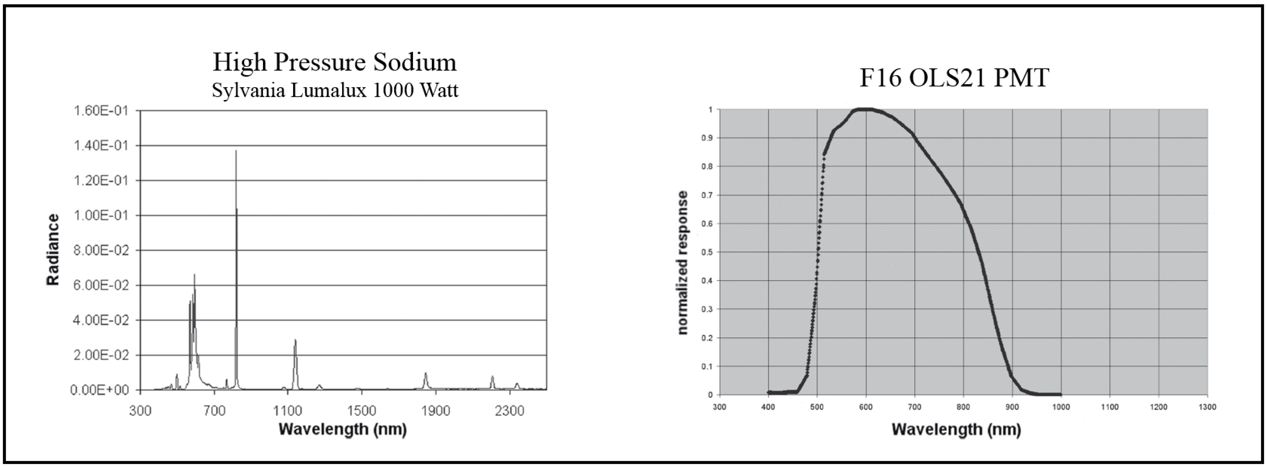
A portable lighting source capable of being observed by the DMSP OLS was built to carry out this study. A number of options were explored, including off the shelf halogen construction lights and off the shelf spot lights. Based on the characteristics of the available lighting types a portable lighting source was designed using commercially available lighting products. High pressure sodium lights, commonly used in warehouses, were chosen for a variety of reasons. High pressure sodium lamps have a very high lumens to watts ratio, so more energy is converted to light
vs. wasted as heat than in common household lamps. Additionally, the spectral emissions from high pressure sodium lamps are highest in the red/orange portion of the visible spectrum (
Figure 1). We measured the spectral signature depicted in
Figure 1 with an ASD field spectrometer (FieldSpec portable spectroradiometer). These measurements were corroborated and validated by Independent Testing Labs Inc [
36] (
Supplementary Figures S1–S4). There is a low amount of Rayleigh scattering due to the red/orange character of these lamps allowing more energy to reach the sensor. The red/orange peak also coincides with the peak of the OLS pre-flight spectral response (
Figure 1).
The high pressure sodium lamps require a ballast, capacitor, and igniter to start the lamp and to regulate the current once the lamp is ignited. For these experiments 250 W lamps and 1000 W lamps were acquired. For the 1000 W lamps the associated ballast, capacitor, and igniter weigh approximately 23 kg each and are designed to hang from a ceiling. In order to direct the light towards the space borne sensor several portable housings were constructed to hold the ballast, capacitor, igniter, and socket housing with the bulb pointed skyward. A 22-inch aluminum shield was mounted to the socket to further direct the light skyward.
Up to eight 1000 W lights could be powered by two 5500 W gas generators. A six foot by ten foot utility trailer was used to transport the portable lighting system and the generators. Six 250 W high pressure sodium lights, eight 1000 W high pressure sodium lights, and two 5500 W generators could be carried inside the trailer.
Figure 1.
Spectral Signature of Lamp and Spectral Response of Defense Meteorological Satellite Programs’ Operational Linescan System (DMSP OLS) F16 sensor.
Figure 1.
Spectral Signature of Lamp and Spectral Response of Defense Meteorological Satellite Programs’ Operational Linescan System (DMSP OLS) F16 sensor.
Note: Figure adapted from Tuttle
et al. 2014 [
37].
The 1000 watt high pressure sodium lamps produce 140,000 lumens. An average 100 watt incandescent household lamp produces 1500 lumens. The 1000 watt lamps used in this study are equivalent to approximately ninety-three 100 watt household incandescent lamps.
2.2. Field Site Selection
It was necessary to select field sites that were completely dark and were not near any sources of light pollution. Selected sites had no observation of light when viewed in the DMSP OLS imagery. This ensured that the portable lighting source was responsible for any light observed in the DMSP OLS data collected during field experiments. The local overpass time of the satellite means that in the summer the sun sets after the overpass. Because of this, the clearest images are collected in the fall, winter, and spring. Most of the field experiments were carried out in the winter, so field sites had to be accessible at all times of year by a truck and 6 foot by 10 foot utility trailer (
Figure 2).
The high pressure sodium lights give off a red/orange light that is viewable from a significant distance. Anecdotal evidence suggests the lights were visible to the human eye from up to 5 miles away across flat land. It is easy to mistake the glow from the portable light source for a wild fire due to the color. Given this it was also important to have permission from local land managers and law enforcement prior to carrying out the field experiments. Consequently site selection was further limited to sites where acquiring the appropriate permissions was possible.
Eventually three sites were chosen (
Figure 3) in Colorado and New Mexico. The sites were on the Pawnee National Grasslands in northeastern Colorado, the Karval State Wildlife Area in eastern Colorado, and the Santa Fe National Forest in northern New Mexico. Each site was easily accessible at all times of year, was far enough from neighboring light sources to be dark in the DMSP OLS data, and permissions from the land managers and local law enforcement were acquired.
Figure 2.
Seven (1000 watt) high pressure sodium lights in the utility trailer and the two generators used to power the lights in the field.
Figure 2.
Seven (1000 watt) high pressure sodium lights in the utility trailer and the two generators used to power the lights in the field.
Using available ephemeris data for the DMSP OLS it was possible to predict the overpass time of the satellite at the different field sites. The predictions proved to be within seconds of the actual overpass times. Field experiments were planned for nights when the lunar illuminance was less than 0.0005 lux and the solar elevation was less than 12 degrees. These requirements ensured there was no moon light or sun light contamination in the imagery during field collections. Weather was also considered and trips were planned for nights that were likely to have clear skies as clouds can obscure the light in the DMSP OLS imagery. Despite planning efforts the weather did not always turn out as predicted. Imagery collected of the field experiments that was found to have cloud cover were excluded from the analysis process.
During each field experiment the portable lighting system was deployed at the site an hour prior to the predicted overpass time. High pressure sodium lights to not achieve their full brightness at ignition. In order to ensure full brightness the lights were turned on at least 45 min prior to the predicted overpass. Although the overpass predictions proved to be accurate within seconds of the actual overpass, the lights were left on for at least 15 min after the predicted overpass to ensure coverage. During the time of the field experiments from December 2009–January 2011 there were two DMSP satellites flying with the OLS onboard (F16 & F18). Depending on the geometry of the satellite on any given night it was possible to have the field site viewed once or twice by each satellite. The portable light was always turned on 45 min or more before the initial predicted overpass and turned off no earlier than 15 min after the last predicted overpass. The entire lighting system was packed up and removed from the sites after every experiment.
Figure 3.
Map of the three field sites in Colorado and New Mexico with a nighttime lights annual composite from satellite F16 for the year 2009 as the background.
Figure 3.
Map of the three field sites in Colorado and New Mexico with a nighttime lights annual composite from satellite F16 for the year 2009 as the background.
2.3. DMSP OLS Data
DMSP OLS data for each field experiment were acquired from the National Geophysical Data Center (NGDC) in Boulder, CO, USA [
38]. The imagery was processed and geolocated in accordance with the methods described in Baugh
et al. [
39] and Elvidge
et al. [
13].
The data acquired came in the form of GeoTiffs and included several images for each orbit. The included images were the visible band imagery, thermal band imagery, samples image, and gain image. The visible image contains digital number (DN) values ranging from 0 to 63. The thermal image contains digital number values ranging from 0 to 255. The samples image contains a value representing the sample in the image and allowed for the calculation of scan angle of each observation. The gain image contains values representing the gain for each pixel in the visible band image and allows for the conversion of the visible image DNs into radiance values.
The OLS data is collected at a resolution of 0.6 km, referred to as fine data. A limited quantity of this data can be recorded between downloads. Additionally, the data is resampled to 2.7 km, by averaging a 5 × 5 grid of fine pixels, onboard the satellite. The resampled data, referred to as smooth data, can be collected globally each day. The Air Force Weather Agency (AFWA) determines where the fine data will be collected at any given time. During this research a request was made to AFWA to collect fine data over the study area and it was granted. During the study, data was collected from both satellites F16 and F18 in both the smooth and fine resolutions.
2.4. Data Analysis
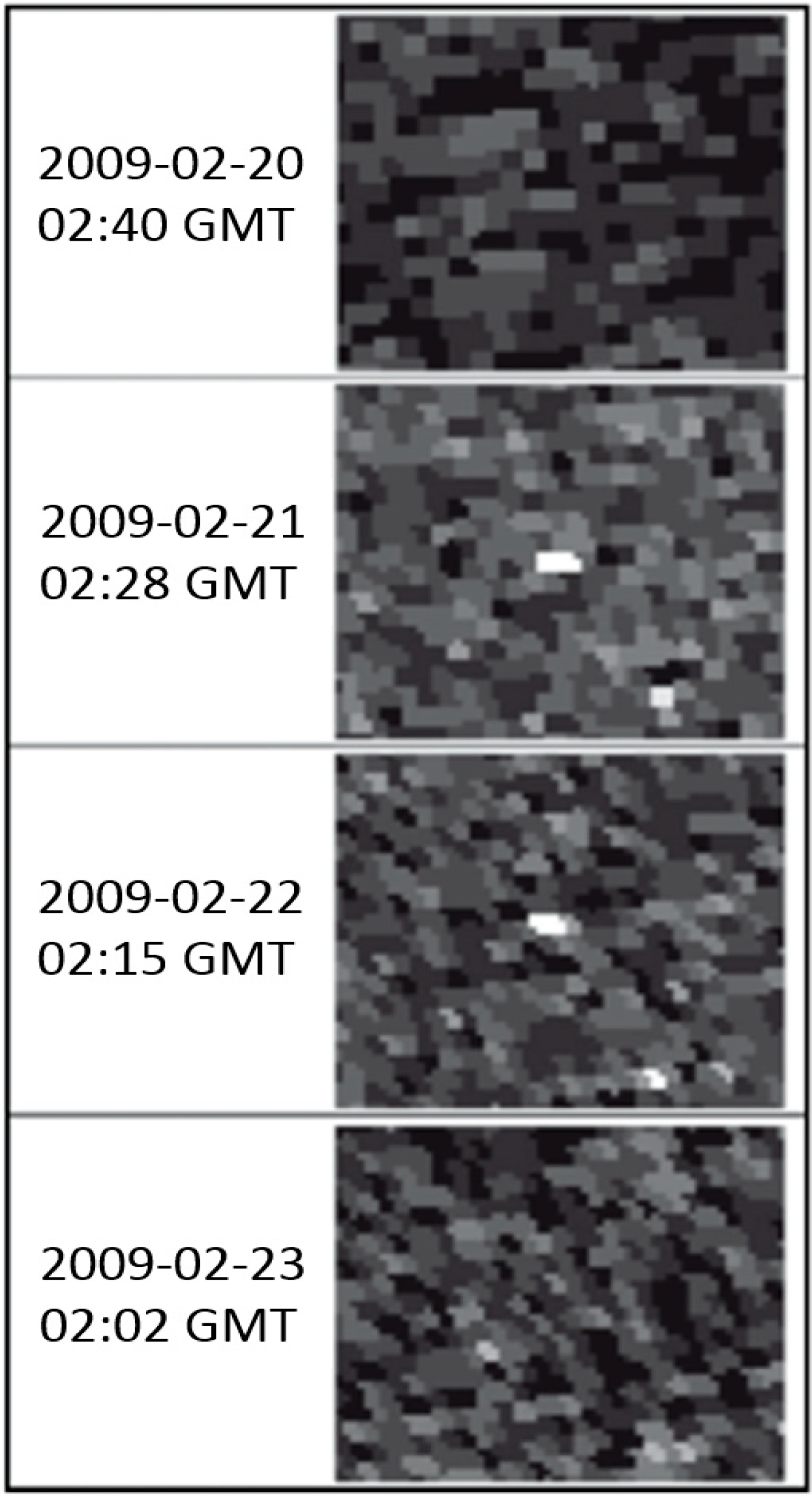
A total of 26 images were collected of the portable lighting source that met all the criteria described in
Section 2.3. Different quantities of light were used on different nights ranging from 1000 W–8000 W. The ground footprint of the OLS is larger than the pixel size [
16] and the portable light source was always detected in multiple pixels. For each image a polygon was created that outlined the pixels in which the portable light source was detected (
Figure 4).
Figure 4.
Example series of DMSP OLS images at Karval Wildlife Area during field collection. These images over four consecutive days which include before, during, and after. Field work (lights on) in the middle (21 February 2009 and 22 February 2009).
Figure 4.
Example series of DMSP OLS images at Karval Wildlife Area during field collection. These images over four consecutive days which include before, during, and after. Field work (lights on) in the middle (21 February 2009 and 22 February 2009).
Using the polygons outlining the light in the imagery the average DN, average gain, and average sample within the polygons were extracted from the visible, sample, and gain images. Using the average DN and average gain, the radiance observed for each collection was calculated. The average sample was used to calculate the average scan angle for each observation of the portable light source. On each night of a field experiment the number of watts of lights used was recorded.
A table was constructed that contained the satellite identifier (F16 or F18), the average scan angle, the watts of light used, and the resolution of the data (fine or smooth). The average scan angle was used to calculate the distance from the portable light source to the sensor to account for optical depth, and this distance was also used to calculate the inverse distance squared.
The table was then imported into JMP® Pro to analyze the data. Linear regression analyses were performed to evaluate the correlation between the brightness of the lights on the ground and the observed data values in the visible band imagery. Although watts are not a measure of brightness it was used here to represent the brightness of the lights used on a given night. Since all the lamps were of the same type (Sylvania Lumalux High Pressure Sodium) the watts were considered to be a valid proxy of the brightness of the lights. The observed radiance was the dependent variable and satellite (nominal), spatial resolution (nominal), brightness of the lights (represented by watts), and optical depth (1/distance to sensor2) were the independent variables.
3. Results and Discussion
3.1. Results of Analysis
During this study different quantities of lamps were used on different nights. The experiments ranged from one 1000 watt lamp up to eight 1000 watt lamps at a time. It was found that eight 1000 watt lamps produce enough energy to saturate the higher resolution fine data collected by the OLS. They did not, however, produce enough energy to saturate the lower resolution smooth data collected by the OLS. One 1000 watt lamp produced enough energy to be detected by the OLS in both the smooth and fine resolution data. This suggests that as few as ninety-three 100 watt incandescent lamps could be observed by the OLS.
The results observed using one 1000 watt lamp suggest that the OLS may be capable of detecting lights producing less energy. It would be valuable to conduct further studies with lamps under 1000 watts. This would allow a confirmation of the minimum detectable brightness of the OLS. Further studies are needed to confirm whether or not one 1000 watt high pressure sodium lamp is the minimum detectable.
Radiance observed by the DMSP OLS is correlated with satellite, spatial resolution, brightness of the lights (represented by watts), and optical depth (1/distance to sensor
2). The results of the linear regression modeling are shown in
Table 1. When attempting to model both satellites F16 and F18 the model resulted in an R
2 of 0.61. Modeling each satellite individually resulted in higher R
2 values, which implies there is a significant difference in current spectral response of the OLS on the two satellites. When modeling satellite F16 the R
2 was 0.72.
Table 1.
Results of Linear Regression Analysis.
Table 1.
Results of Linear Regression Analysis.
| Satellite | Equation | Rsquare |
|---|
| F16 & F18 | Radiance = 1.4296e−7 + 1.38e−12 * Watts + (−0.172516 * 1/OD2) + (−1.138e−9 * Sat[F16]) + (−7.014e−8 * Resolution[Smooth]) | 0.614165 |
| F16 | Radiance = 2.816e−7 + 1.38e−12 * Watts + (−0.172516 * 1/OD2) + (−7.83e−8 * Resolution[Smooth]) | 0.722657 |
| F18 | Radiance = 6.2462e−8 + 1.573e−11 * Watts + (−0.011343 * 1/OD2) + (−6.008e−8 * Resolution[Smooth]) | 0.717696 |
3.2. Accuracies, Errors, and Uncertainties
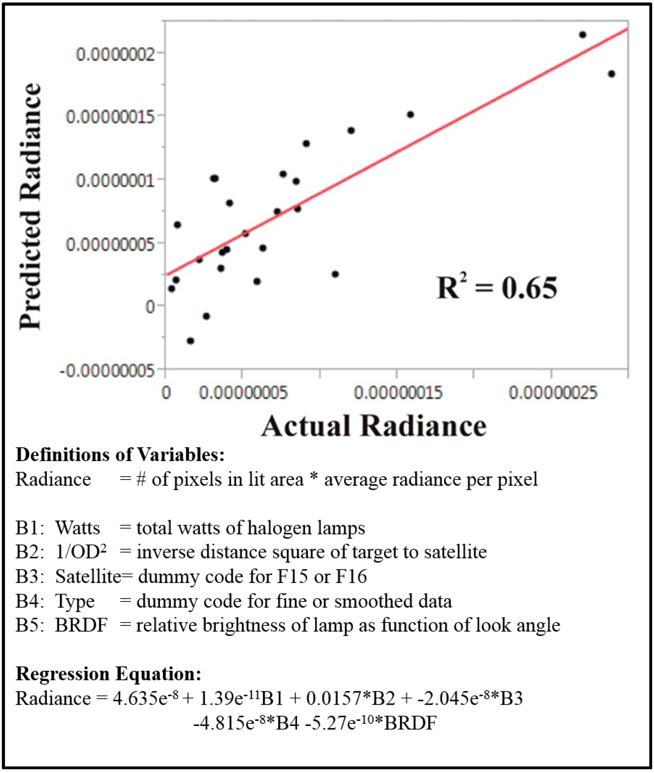
We have demonstrated the reassuring truth that the strength of the signal observed by the DMSP OLS sensor is a function of the brightness of the lights at the surface. The regression models (
Table 1 and
Figure 5) suggest that we can explain 60%–70% of the variation of signal at the sensor from basic physical models that use the following simple variables: Watts of radiation in the range of wavelengths that the sensor responds to, Optical Depth derived by geometry of satellite look angle, a nominal satellite variable, and a nominal smooth or fine resolution variable. The models show that satellite, resolution, brightness of the lights, and optical depth explain much of the variability in radiance observed by the OLS. It is expected that some portion of the unexplained variability is due to degradation of the sensor between December 2009 and January 2011. However, the degradation over that time may not account for all of the unexplained variation. Each night the thermal data from the OLS was examined to determine if the observation is cloud free. However, there is a chance that very light clouds could go undetected by the OLS and could have an impact on the observed DN. It is possible that using an atmospheric model in addition to optical depth would account for some of the unexplained variability. Very low signal will suffer from an even larger percentage error when there are clouds present. Fortunately most of our observations were not at low signal levels. Very high signal actually saturates the DMSP OLS sensor and these regression equations are not capable of correcting for saturated areas that are typical in the urban cores of major population centers. For historical work there have been many approaches explored for dealing with saturation in the urban cores [
40,
41,
42]. For future work the VIIRS instrument has a significantly larger dynamic range and the saturation problem is virtually non-existent for imagery derived from VIIRS.
Another factor that may account for some of unexplained variability is the oblong shape of the lamps used in these experiments. It is expected that the emitted energy of the lamps is not consistent from all angles. We took the lamps to a lab to measure the Bidirectional Reflectance Distribution Function (BRDF) (
Supplementary Figures S1–S4). We used the BRDF information in conjunction with scan angle as an additional variable in the regression to predict radiance but this accounted for only a small fraction of the unexplained variability (
Figure 5). In fact, the parameter for the effect of the BRDF was not even significant although it improved the R
2 marginally. Lastly, the smooth data pixels are created by averaging a five pixel by five pixel grid of fine data. Depending on where the grids fall in the data the resulting radiance in the smooth data can be very different. For example, if the five by five grid was centered on the brightest fine pixels the resulting smooth pixel would have a high DN. However, if multiple five by five grids share the brightest fine pixels the resulting smooth pixels would have a lower DN. This process is certainly the cause of some of the unexplained variability.
Figure 5.
Results of Linear Regression incorporating Angular Variation of Light Intensity (BRDF).
Figure 5.
Results of Linear Regression incorporating Angular Variation of Light Intensity (BRDF).
3.3. Discussion
Given the correlation between the brightness of the portable light source and the observed radiance this process should be valuable for radiance calibration. By deploying a light source of this type at a known location over long periods a record of the sensor response could be created. This record would allow for the creation of offsets to account for changes in spectral response of the OLS over time. Additionally, it would allow for offsets to account for differences in spectral response between two or more satellites with the OLS on board. These offsets would allow for more precise temporal and inter-satellite comparisons of OLS nighttime lights data. It would be valuable to have a location, with no surrounding lights, capable of supporting a long term installation of a light source of this nature.
In addition to the applicability of this process to the DMPS OLS, there are other applications. The recently launched Visible Infrared Imager Radiometer Suite (VIIRS) onboard NASA’s Suomi National Polar-orbiting Operational Environmental Satellite System Preparatory Project (NPP) spacecraft would also benefit from the process defined here. VIIRS acquired its first measurements on 21 November 2011 [
43] and is capable of low light imaging collection to produce nighttime lights imagery, similar to the DMSP OLS. Temporal and inter-satellite comparisons of VIIRS data would benefit from the portable light design and calibration process as well.
This process would also be applicable and beneficial to the proposed NightSat mission concept [
44,
45]. The NightSat proposes a new sensor capable of global observations collected at a spatial resolution capable of delineating primary features of human settlements. This sensor also includes increased spectral resolution that would allow it to distinguish between different types of lamps, for example, distinguishing high pressure sodium from metal halide. To take advantage of this characteristic of NightSat, it would be valuable to include multiple lamp types in the process described here to increase the relevance.
Lastly, this methodology also has applications to nighttime photographs taken from the International Space Station (ISS) at night [
46]. Astronauts onboard the ISS are able to take photos at night that present varying resolution color images of nighttime lights. These photographs are a valuable addition to satellite nighttime lights imagery for a wide array of research topics. Like the proposed NightSat these photos allow one to observe light sources with different spectral signatures. The process described here should be valuable for these ISS photos as well.
4. Conclusions
A portable light source capable of detection by the DMSP OLS was designed and fielded on 27 nights between December 2009 and January 2011. The light was deployed in locations with no surrounding light sources, on nights with a lunar illuminance less than 0.0005 lux and a solar elevation angle less than 12 degrees. On 13 of those nights, cloud free imagery was collected with observations of the portable light source. The portable light was used in multiple lamp configurations ranging from one 1000 watt lamp to eight 1000 watt lamps. It was established that eight 1000 watt high pressure sodium lamps produce enough energy to saturate the fine resolution data, but not the smooth resolution data. Furthermore, it was determined that the DMSP OLS can detect as little as one 1000 watt high pressure sodium lamp.
DMSP OLS data was collected and acquired for the nights of the field experiments. The DN values were converted to radiance using the pre-flight spectral response of the OLS and the sensor gain at the time of collection. Linear regression was used to model radiance with the following parameters: satellite (nominal), spatial resolution (nominal), brightness of the lights (represented by watts), and optical depth (1/distance to sensor2). A strong correlation between these variables and radiance was discovered.
This methodology can be used to improve temporal and inter-satellite comparisons if deployed at regular intervals. Moreover, this process should have relevance for both the VIIRS sensor and the proposed NightSat sensor and may improve the utility of nighttime photographs taken from the International Space Station. The results indicate that finding a dark location capable of leaving a similar lighting system deployed long term would be of significant value for nighttime lights research and applications.
Future research in several areas is indicated. Field experiments should be conducted with lamps producing less energy than one 1000 watt high pressure sodium lamp. This would allow the minimum detectable brightness to be soundly defined. In addition, a detailed atmospheric model for each night of observation might improve the models. Lastly, a campaign carried out at regular intervals with the same number of lamps on each night would be valuable. The results suggest that such a campaign would allow for offsets accounting for sensor degradation and differences between the sensitivity of the OLS on different satellites to be accounted for. This would allow for improvements in the results of studies using temporal and inter-satellite data comparisons.
Supplementary Files
Supplementary File 1Acknowledgments
This research was funded in part by and NASA Earth Space Science Fellowship and an ASPRS Rocky Mountain Region Scholarship. The authors wish to thank Warren Cummings (Colorado Division of Wildlife), James Munoz (National Forest Service), and Vernon Koehler (National Forest Service) for their support to this study related to the field sites. Additionally, the authors wish to thank all the individuals (Kristina Yamamoto, Andy Tennant, Brenton Wonders, Warren Wonders, Anna Talucci, Sammy Lester, and Austin Shull) who assisted in the various field expeditions. Finally, this research could not have been completed without the cooperation and assistance of the Air Force Weather Agency.
Author Contributions
Benjamin Tuttle, Paul Sutton, Chris Elvidge and Sharolyn Anderson conceived and designed the experiments. Mainly, Benjamin Tuttle performed the experiments with the assistance of Kim Baugh, Paul Sutton and Sharolyn Anderson. Benjamin Tuttle, Paul Sutton and Kim Baugh analyzed the data. Tilottama Ghosh contributed analysis tools and model verification. Benjamin Tuttle, Tilottama Ghosh, and Paul Sutton wrote the paper with edits from Chris Elvidge and Sharolyn Anderson.
Conflicts of Interest
The authors declare no conflict of interest.
References
- Chand, T.R.K.; Badarinath, K.V.; Prasad, V.K.; Murthy, M.S.R.; Elvidge, C.D.; Tuttle, B.T. Monitoring forest fires over the Indian region using Defense Meteorological Satellite Program-Operational Linescan System nighttime satellite data. Remote Sens. Environ. 2006, 103, 165–178. [Google Scholar] [CrossRef]
- Chand, T.R.K.; Badarinath, K.V.S.; Murthy, M.S.R.; Rajshekhar, G.; Elvidge, C.D.; Tuttle, B.T. Active forest fire monitoring in Uttaranchal state, India using multi-temporal DMSP-OLS and MODIS data. Int. J. Remote Sens. 2007, 28, 2123–2132. [Google Scholar] [CrossRef]
- Cova, T.J.; Sutton, P.C.; Theobald, D.M. Exurban change detection in fire-prone areas with nighttime satellite imagery. Photogramm. Eng. Remote Sens. 2004, 70, 1249–1257. [Google Scholar] [CrossRef]
- Elvidge, C.D.; Baugh, K.E.; Hobson, V.R.; Kihn, E.A.; Kroehl, H.W. Detection of fires and power outages using DMSP-OLS data. In Remote Sensing Change Detection: Environmental Monitoring Methods and Applications; Lunetta, R.S., Elvidge, C.D., Eds.; Ann Arbor Press: Chelsea, MI, USA, 1998; pp. 123–135. [Google Scholar]
- Elvidge, C.D.; Hobson, V.R.; Baugh, K.E.; Dietz, J.B.; Shimabukuro, Y.E.; Krug, T.; Novo, E.; Echavarria, F.R. DMSP-OLS estimation of tropical forest area impacted by surface fires in Roraima, Brazil: 1995 versus 1998. Int. J. Remote Sens. 2001, 22, 2661–2673. [Google Scholar] [CrossRef]
- Elvidge, C.D.; Nelson, I.; Hobson, V.R.; Safran, J.; Baugh, K.E. Detection of fires at night using DMSP-OLS data. In Global and Regional Vegetation Fire Monitoring from Space: Planning a Coordinated International Effort; Ahern, F.J., Goldammer, J.G., Justice, C.O., Eds.; SPB Academic Publishing: The Hague, The Netherlands, 2001; pp. 125–144. [Google Scholar]
- McNamara, D.; Stephens, G.; Ramsay, B.; Prins, E.; Csiszar, I.; Elvidge, C.; Hobson, R.; Schmidt, C. Fire detection and monitoring products at the National Oceanic and Atmospheric Administration. Photogramm. Eng. Remote Sens. 2002, 68, 774–775. [Google Scholar]
- Elvidge, C.D.; Baugh, K.; Tuttle, B.; Ziskin, D.; Ghosh, T. Satellite observation of heavily lit fishing boat activity in the coral triangle region. In Proceedings of the 30th Asian Conference on Remote Sensing, Beijing, China, 18–23 October 2009.
- Maxwell, M.R.; Henry, A.; Elvidge, C.D.; Safran, J.; Hobson, V.R.; Nelson, I.; Tuttle, B.T.; Dietz, J.B.; Hunter, J.R. Fishery dynamics of the California market squid (Loligo opalescens), as measured by satellite remote sensing. Fish. Bull. 2004, 102, 661–670. [Google Scholar]
- Nagatani, I. A methodology to create DMSP-OLS night-time mosaic image for monitoring fishing boats. In Proceedings of the 2010 Asia-Pacific Advanced Network Meeting, Hanoi, Vietnam, 9–13 August 2010; pp. 143–152.
- Elvidge, C.D.; Erwin, E.H.; Baugh, K.E.; Tuttle, B.T.; Howard, A.T.; Pack, D.W.; Milesi, C. Satellite data estimate worldwide flared gas volumes. Oil Gas J. 2007, 105, 50–58. [Google Scholar]
- Elvidge, C.D.; Ziskin, D.; Baugh, K.E.; Tuttle, B.T.; Ghosh, T.; Pack, D.W.; Erwin, E.H.; Zhizhin, M. A fifteen year record of global natural gas flaring derived from satellite data. Energies 2009, 2, 595–622. [Google Scholar] [CrossRef]
- Elvidge, C.D.; Imhoff, M.L.; Baugh, K.E.; Hobson, V.R.; Nelson, I.; Safran, J.; Dietz, J.B.; Tuttle, B.T. Night-time lights of the world: 1994–1995. ISPRS J. Photogramm. Remote Sens. 2001, 56, 81–99. [Google Scholar] [CrossRef]
- Elvidge, C.D.; Baugh, K.E.; Kihn, E.A.; Kroehl, H.W.; Davis, E.R. Mapping city lights with nighttime data from the DMSP operational linescan system. Photogramm. Eng. Remote Sens. 1997, 63, 727–734. [Google Scholar]
- Small, C.; Pozzi, F.; Elvidge, C.D. Spatial analysis of global urban extent from DMSP-OLS night lights. Remote Sens. Environ. 2005, 96, 277–291. [Google Scholar] [CrossRef]
- Elvidge, C.D.; Safran, J.; Nelson, I.L.; Tuttle, B.T.; Hobson, V.R.; Baugh, K.E.; Dietz, J.B.; Erwin, E.H. Area and position accuracy of DMSP nighttime lights data. In Remote Sensing and GIS Accuracy Assessment; Lunetta, R.S., Lyon, J.G., Eds.; CRC Press: Boca Raton, FL, USA, 2004; pp. 281–292. [Google Scholar]
- Witmer, F.D.W.; O’Loughlin, J. Detecting the effects of wars in the Caucasus regions of Russia and Georgia using radiometrically normalized DMSP-OLS nighttime lights imagery. GISci. Remote Sens. 2011, 48, 478–500. [Google Scholar] [CrossRef]
- NOAA. Global Radiance Calibrated Nighttime Lights. Available online: http://ngdc.noaa.gov/eog/dmsp/download_radcal.html (accessed on 2 December 2014).
- Doll, C.N.H.; Muller, J.P.; Elvidge, C.D. Night-time imagery as a tool for global mapping of socioeconomic parameters and greenhouse gas emissions. AMBIO J. Human Environ. 2000, 29, 157–162. [Google Scholar]
- Ghosh, T.; Elvidge, C.D.; Sutton, P.C.; Baugh, K.E.; Ziskin, D.; Tuttle, B.T. Creating a global grid of distributed fossil fuel CO2 emissions from nighttime satellite imagery. Energies 2010, 3, 1895–1913. [Google Scholar] [CrossRef]
- Letu, H.; Nakajima, T.Y.; Nishio, F. Regional-scale estimation of electric power and power plant CO2 emissions using DMSP/OLS nighttime satellite data. Environ. Sci. Technol. Lett. 2014, 1, 259–265. [Google Scholar] [CrossRef]
- Prasad, V.K.; Kant, Y.; Gupta, P.K.; Elvidge, C.; Badarinath, K.V.S. Biomass burning and related trace gas emissions from tropical dry deciduous forests of India: A study using DMSP-OLS data and ground-based measurements. Int. J. Remote Sens. 2002, 23, 2837–2851. [Google Scholar] [CrossRef]
- Elvidge, C.D.; Sutton, P.C.; Ghosh, T.; Tuttle, B.T.; Baugh, K.E.; Bhaduri, B.; Bright, E. A global poverty map derived from satellite data. Comput. Geosci. 2009, 35, 1652–1660. [Google Scholar] [CrossRef]
- Ghosh, T.; Powell, R.; Elvidge, C.D.; Baugh, K.E.; Sutton, P.C.; Anderson, S. Shedding light on the global distribution of economic activity. Open Geogr. J. 2010, 3, 148–161. [Google Scholar]
- Ghosh, T.; Powell, R.L.; Anderson, S.; Sutton, P.C.; Elvdige, C.D. Informal economy and remittance estimates of India using nighttime imagery. Int. J. Ecol. Econ. Stat. 2010, 17, 16–50. [Google Scholar]
- Elvidge, C.D.; Sutton, P.C.; Wagner, T.W.; Ryzner, W.; Vegelman, J.E.; Goetz, S.J.; Smith, A.J.; Jantz, C.; Seto, K.C.; Imhoff, M.L.; Gutman, G.; et al. Urbanization. In Land Change Science; Gutman, G., Janetos, A.C., Justice, C.O., Moran, E.F., Mustard, J.F., Rindfuss, R.R., Skole, D., Turner, B.L., II, Cochrane, M.A., Eds.; Kluwer Academic Publishers: Norwell, MA, USA, 2004; pp. 315–328. [Google Scholar]
- Elvidge, C.D.; Tuttle, B.T.; Sutton, P.C.; Baugh, K.E.; Howard, A.T.; Milesi, C.; Bhaduri, B.L.; Nemani, R. Global distribution and density of constructed impervious surfaces. Sensors 2007, 7, 1962–1979. [Google Scholar] [CrossRef]
- Henderson, M.; Yeh, E.T.; Gong, P.; Elvidge, C.; Baugh, K. Validation of urban boundaries derived from global night-time satellite imagery. Int. J. Remote Sens. 2003, 24, 595–609. [Google Scholar] [CrossRef]
- Imhoff, M.L.; Lawrence, W.T.; Elvidge, C.D.; Paul, T.; Levine, E.; Privalsky, M.V.; Brown, V. Using nighttime DMSP/OLS images of city lights to estimate the impact of urban land use on soil resources in the United States. Remote Sens. Environ. 1997, 59, 105–117. [Google Scholar] [CrossRef]
- Imhoff, M.L.; Lawrence, W.T.; Stutzer, D.C.; Elvidge, C.D. A technique for using composite DMSP/OLS “city lights” satellite data to map urban area. Remote Sens. Environ. 1997, 61, 361–370. [Google Scholar] [CrossRef]
- Lo, C.P. Modeling the population of China using DMSP operational linescan system nighttime data. Photogramm. Eng. Remote Sens. 2001, 67, 1037–1047. [Google Scholar]
- Lo, C.P. Urban indicators of China from radiance-calibrated digital DMSP-OLS nighttime images. Ann. Assoc. Am. Geograph. 2002, 92, 225–240. [Google Scholar] [CrossRef]
- Potere, D.; Schneider, A. A critical Look at representations of urban areas in global maps. GeoJournal 2007, 69, 55–80. [Google Scholar] [CrossRef]
- Sutton, P.C.; Elvidge, C.; Obremski, T. Building and evaluating models to estimate ambient population density. Photogramm. Eng. Remote Sens. 2003, 69, 545–553. [Google Scholar] [CrossRef]
- Anderson, S.J.; Tuttle, B.T.; Powell, R.L.; Sutton, P.C. Characterizing relationships between population density and nighttime imagery for Denver, Colorado: issues of scale and representation. Int. J. Remote Sens. 2010, 31, 5733–5746. [Google Scholar] [CrossRef]
- Independent Testing Labs Inc. Available online: www.itlboulder.com (accessed on 2 December 2014).
- Tuttle, B.T.; Anderson, S.J.; Sutton, P.C.; Elvidge, C.D.; Baugh, K. It used to be dark here. Geolocation calibration of the defense meteorological satellite program operational linescan system. Photogram. Eng. Remote Sens. 2013, 79, 287–297. [Google Scholar] [CrossRef]
- NOAA/NGDC Earth Observation Group. Defense Meteorological Satellite Program. Available online: http://ngdc.noaa.gov/eog/dmsp.html (accessed on 2 December 2012).
- Baugh, K.; Elvidge, C.; Ghosh, T.; Ziskin, D. Development of a 2009 Stable Lights Product Using DMSP-OLS data. In Proceedings of the 30th Asia-Pacific Advanced Network Meeting, Hanoi, Vietnam, 9–13 August 2010; pp. 114–130.
- Cao, X.; Chen, J.; Imura, H.; Higashi, O. A SVM-based method to extract urban areas from DMSP-OLS and SPOT VGT data. Remote Sens. Environ. 2009, 113, 2205–2209. [Google Scholar] [CrossRef]
- Letu, H.; Hara, M.; Tana, G.; Nishio, F. A saturated light correction method for DMSP/OLS nighttime satellite imagery. IEEE Trans. Geosci. Remote Sens. 2012, 50, 389–396. [Google Scholar] [CrossRef]
- Zhang, Q.; Schaaf, C.; Seto, K.C. The vegetation adjusted NTL urban index: A new approach to reduce saturation and increase variation in nighttime luminosity. Remote Sens. Environ. 2013, 129, 32–41. [Google Scholar] [CrossRef]
- NASA. NASA’s NPP Satellite Acquires First VIIRS Image. Available online: http://www.nasa.gov/mission_pages/NPP/news/viirs-firstlight.html (accessed on 2 December 2014).
- Elvidge, C.D.; Cinzano, P.; Pettit, D.R.; Arvesen, J.; Sutton, P.; Small, C.; Nemani, R.; Longcore, T.; Rich, C.; Safran, J.; et al. The Nightsat mission concept. Int. J. Remote Sens. 2007, 28, 2645–2670. [Google Scholar] [CrossRef]
- Elvidge, C.D.; Safran, J.; Tuttle, B.; Sutton, P.; Cinzano, P.; Pettit, D.; Arvesen, J.; Small, C. Potential for global mapping of development via a nightsat mission. GeoJournal 2007, 69, 45–53. [Google Scholar] [CrossRef]
- Lulla, K. Nighttime urban imagery from international space station: Potential applications for urban analyses and modeling. Photogramm. Eng. Remote Sens. 2003, 69, 941–942. [Google Scholar]
© 2014 by the authors; licensee MDPI, Basel, Switzerland. This article is an open access article distributed under the terms and conditions of the Creative Commons Attribution license (http://creativecommons.org/licenses/by/4.0/).


