1. Introduction
Airborne light detection and ranging (lidar), also called airborne laser scanning, has become a powerful support for spatial data acquisition over the past decades. Lidar is capable of rapidly gathering geospatial data of the ground surface by emitting and receiving laser pulses, and its measurements are not influenced by illumination conditions. Compared with traditional field surveying and photogrammetric methods, lidar has obvious advantages, e.g., high precision and great density, especially in some difficult areas such as forest, desert, and beach [
1,
2,
3]. It is therefore widely exploited to produce the high-resolution digital terrain model (DTM), which is necessary for numerous geospatial applications and analysis [
4,
5,
6].
Although the use of the lidar system is becoming increasingly popular, the effective processing of raw data remains a big challenge [
7,
8]. Raw lidar data mainly consist of huge point clouds without classification information. These point clouds may contain diverse objects, such as vegetation, buildings, vehicles, and electrical wires. Hence, the crucial step in DTM generation is to eliminate nonground points from the obtained point cloud; this process is referred to as filtering [
9,
10]. Automatic lidar data filtering has been a considerably difficult task, especially for large areas with changing terrain, because of the complex configuration and geometrical similarities of ground and nonground objects [
10,
11,
12,
13,
14,
15].
Many researchers have explored various approaches to deal with lidar data filtering [
10,
11,
12,
13,
16,
17]. Slope-based approaches calculate the slopes between neighboring points using a predefined threshold for filtering because slopes between nonground and bare ground points are distinct [
2,
18,
19,
20,
21]. Directional scanning approaches inspect slopes and elevation differences to identify ground points along a one-dimensional scan line in a specified direction [
1,
2,
19,
22,
23]. Surface interpolation approaches and triangular irregular network (TIN) densification approaches progressively approximate ground surfaces by considering the constraints of angle and distance [
24,
25,
26,
27,
28,
29]. A hierarchical approach is combined with surface interpolation approaches in some studies to enhance processing efficiency [
30]. Mongus and Žalik [
31] interpolated coarse surface towards the terrain from the top to the bottom of the hierarchy by the iterative thin plate spline, and the thresholds were defined based on the standard deviation of points’ residuals from the surface. Morphological approaches use morphological operations such as openings to separate grounds and objects [
9,
13,
32,
33,
34,
35]. Morphological approaches have simple concepts and can be easily implemented [
33]. Moreover, many studies have demonstrated that this group of approaches can properly remove object points [
9,
33,
36,
37]. Zhang
et al. [
9] calculated the height differences of original and morphologically opened surfaces, compared them with a predefined threshold, and progressively distinguished nonground points with gradually increasing window sizes. Chen
et al. [
33] developed a morphological filter by assuming that the slope is inconstant. Li
et al. [
38] redefined morphological opening by the feature points with dramatic height changes. Because objects were most likely to appear around the feature points, morphological erosion and dilation were only performed on the nearby points of the feature points. This could reduce the possibility of cutting the smooth terrain with a gradual height change. Then a region growing approach was used to recall the removed points that were attached to other ground points. The use of existing approaches has achieved some success, but the filtering results for difficult landscapes, especially for complex urban and highly steep areas, are not completely reliable [
1,
8,
31,
39].
The present study proposes an improved top-hat filter with a sloped brim for obtaining ground points from raw lidar point clouds. A sloped brim filter extending outward from the obtained top hats is designed to enhance the robustness of the method for complex objects and terrains.
Section 2 explains the basic principles and implementation procedure of this algorithm.
Section 3 describes and analyzes the experimental results.
Section 4 concludes the study.
2. Methodology
This section is divided into three subsections to explain the methodology.
Section 2.1 introduces the classic top-hat transformation, which is the kernel commonly used in many morphological filters. The focus of the proposed method is on promoting its robustness for complex terrains and objects through the addition of an extending brim filter to the classic top-hat transformation.
Section 2.2 illustrates the principle of the improved top-hat filter with a sloped brim.
Section 2.3 presents the detailed implementation procedure.
2.1. Classic Top-Hat Filter
The morphological opening operation is widely used to flatten the components of a grayscale image that are brighter than the background. The operation can also be used in lidar filtering to remove the objects that are higher than the surrounding ground. The opening operation involves two basic morphological operations, erosion and dilation. Erosion obtains the smallest value within a two-dimensional window, also called structuring element (SE), whereas dilation acquires the largest value within the SE. The erosion and dilation of input set
f using SE
B are denoted by
εB (
f) and
δB (
f), respectively. The opening of input set
f using SE
B is calculated as follows:
Then, the morphological top-hat transformation TH
B (
f) is calculated as follows:
Figure 1 illustrates the classic top-hat transformation.
Figure 1b and
Figure 1c show the result of
f eroded by SE
B and the result of dilation by the same SE after erosion, respectively.
Figure 1a–c show that the initial erosion removes the objects that are smaller than the used SE, but it also cuts the high-relief terrain such as the partial terrain in the blue circle in
Figure 1b. The subsequent dilation again retrieves the high-relief terrain, which is larger than the SE, without reintroducing the objects totally removed by erosion. Hence, the opening operation is usually applied to remove small objects with respect to the size of the SE in practical applications. However, some rugged terrain may also be removed, as shown in
Figure 1c. The difference between the original surface and the opened surface should be compared which is the function of the top-hat transformation.
Figure 1d shows the removed protrusions that are divided into aboveground objects and rugged terrain by thresholding.
Figure 1.
Example of the classic top-hat transformation: (a) input set f and SE; (b) erosion result; (c) result of dilation after erosion; (d) extracted top-hats.
Figure 1.
Example of the classic top-hat transformation: (a) input set f and SE; (b) erosion result; (c) result of dilation after erosion; (d) extracted top-hats.
The top-hat transformation returns a set of the objects that are smaller than the SE and higher than the surrounding surface (
Figure 1). The sizes of the objects removed depend on the specified SE. Small SEs can only be used to remove small objects, whereas large SEs are needed to remove large objects. Meanwhile, steeply protruding terrains are easily flattened. Some researchers have thus adopted a series of increasing window sizes and thresholds to eliminate objects of various sizes [
9,
11,
18]. However, determining whether the height differences in the top-hat transformation are caused by nonground objects or by the variations in the terrain relief remains a challenge in complex landscapes, especially when using large windows on abrupt terrains [
1,
8,
10,
12,
14,
31,
33].
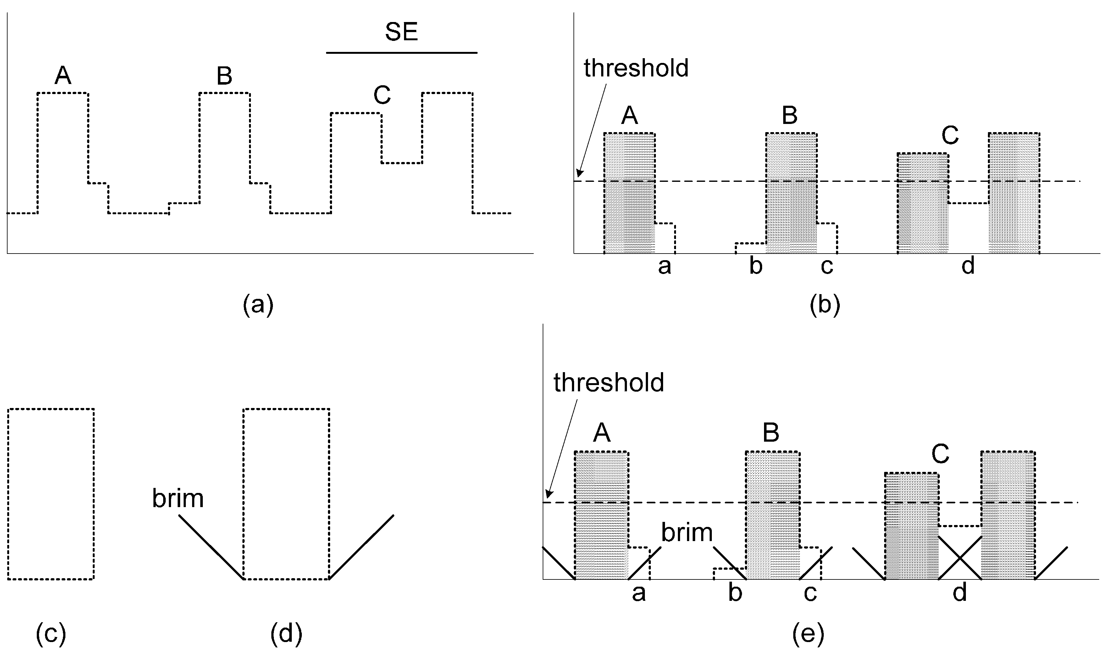
2.2. Improved Top-Hat Filter with Sloped Brim
For three-dimensional lidar point clouds, nonground objects are mainly identified by the distinct elevation discontinuities of point clouds caused by objects. Gradient is a measure of the intensity of elevation change between neighboring points. Morphological gradients obtained using symmetrical SEs have little dependence on the directionality of elevation changes. This characteristic makes morphological gradients suitable for irregularly distributed lidar points. Gradients can be expressed numerically by mathematical morphology in several ways [
40]. Two kinds of morphological gradients are used in the proposed filter,
i.e., internal gradient and external gradient.
The internal gradient of a considered point is denoted by
ρ− using the elementary SE
B (3 × 3 square):
Internal gradients represent the descending extent of point elevation in the neighborhood. External gradients
ρ+ represent the ascending extent of point elevation in the neighborhood and are calculated as
Adaptin
g the size of the used windows is necessary to eliminate nonground objects of different sizes by top-hat filter. The height difference threshold for top hats must be large to avoid the omission of rugged terrains when using large windows. Some complex objects (e.g., the multilayer buildings in
Figure 2a under this strategy. In complicated urban environments, the structures of buildings vary greatly. A large threshold is needed to remove large buildings, such as buildings A, B, and C in
Figure 2b, while low layers, such as parts a, c, and d in
Figure 2b, cannot be identified.
Figure 2d shows an improved top-hat transformation designed to solve this problem. Unlike the traditional top-hat shape, the improved top hat has a sloped brim extending outward around the boundary of the hat.
Figure 2e considers parts a, b, c, and d using the improved top-hat filter.
To simplify implementation, the brim filtering is executed along the rows and columns from left to right and then from bottom to top on an index grid. Every top hat on every row or column is firstly located, and then the brims start from the edge of the top hat and extend outward along the row or column. A brim extends until meeting a point under one of the following three conditions: (a) the difference of original and opened heights of the point is not larger than a defined threshold, (b) the point has outstanding internal gradient, and (c) the point belongs to another top hat. The brim is judged as ground if meeting the above condition (a), otherwise the brim is judged as a nonground object if meeting the above condition (b) or (c). Therefore, for a considered brim on a row or column, its covered continuous points are judged as nonground points if those points meet the following condition:
where
i ∈ [1, 2, …, n],
dhi is the difference of original and opened heights of the
ith lidar point derived by top-hat transformation,
Thbrim(i) is the height difference threshold of the
ith point defined in Equation (6),
Dist(0) is the distance between the beginning point and the top hat derived by thresholding (
Figure 2b), and
ρ−(n) is the internal gradient of the ending point. To simplify the computation, the distance
Dist(
i) is measured by the number of grid cells:
where
a is a coefficient used to set the tolerance of the height difference of the terrain relief near objects. This coefficient is set to 1 for the dataset tested in this study.
Figure 2e shows that parts a, c, and d are eliminated through brim filtering while part b is preserved as terrain.
In order to clarify the above procedure, the pseudo code along a row on the index grid is as follows:
Step 1) Search a series of continuous grid cells belonging to a top hat.
Step 2) /* the brim extends outward from the left side*/
for gridCell = startCell−1 → 0
for every point∈gridCell
if (dh(point)>Thbrim(point))
mark the point belonging to the brim
if (dh(point)≤Thbrim(point))
mark all points of the brim as ground;
end for brim extending.
if (ρˉ(point)>Thbrim(point) OR point∈another top hat)
mark all points of the brim as nonground;
end for brim extending.
end
end
Step 3) /* the brim extends outward from the right side */
for gridCell = endCell+1 → gridWidth−1
for every point∈gridCell
if (dh(point)>Thbrim(point))
mark the point belonging to the brim
if (dh(point)≤Thbrim(point))
mark all points of the brim as ground;
end for brim extending.
if (ρ−(point)>Thbrim(point) OR point∈another top hat)
mark all points of the brim as nonground;
end for brim extending.
end
end
Step 4) If there are other top hats to consider, go to step 1;
otherwise, exit.
Here, startCell and endCell are the starting and ending grid cells belonging to a top hat along a row of the index grid, gridCell is the current grid cell reached by the brim’s extension, gridWidth is the number of grid cells of every row, point refers to the lidar points contained in gridCell, dh(point) is the difference of the original and opened heights of point, and Thbrim(point) denotes the threshold defined by Equation (6). After the brim filtering is executed along the rows as above, the procedure is executed likewise along the columns.
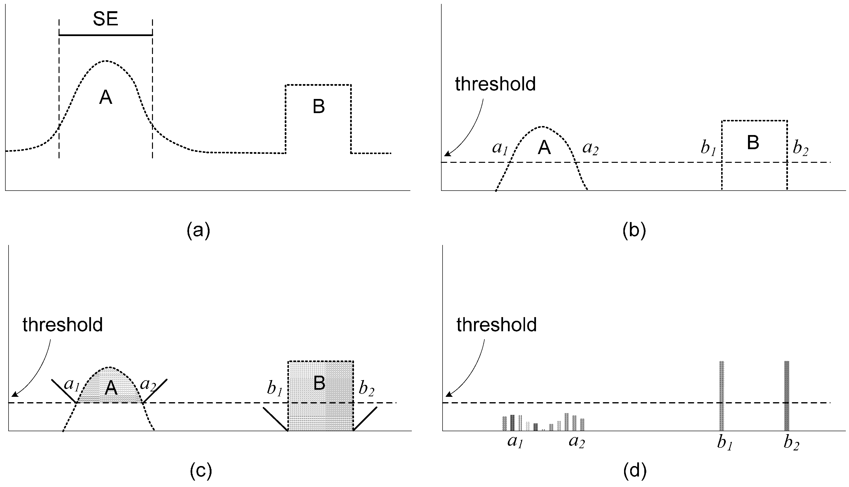
Although the classic top-hat transformation with thresholding can suppress the omission error for rugged terrains, the protruding terrain features are probably flattened at the sites where abrupt relief occurs (e.g., the case in
Figure 3a). Protruding ground A and building B both have a significant height difference. Hence, differentiating them by thresholding top hats is impossible. In the improved top hat with brim, the transitions of the top hats and brims are obviously very different (
Figure 3c). The transitions of the top hat and brim are smooth at location
a1,
a2 for protruding ground A, and steep at location
b1,
b2 for building B. The elevation change intensity at transitions can be measured by comparing the elevations between the edge points and the beginning points of the brim. This comparison is a function of morphological internal gradients.
Figure 3d shows that the internal gradients of the edge points of protruding ground A are relatively small, whereas those of building B are outstanding.
Figure 2.
Example of the improved top-hat filter with a sloped brim for identifying complex objects with multilayer structures: (a) original point set; (b) results by top-hat transformation (gray portions represent the parts extracted by thresholding the top hats); (c) shape of classic top-hat filter; (d) shape of improved top-hat filter with sloped brim; (e) suspicious parts inspected by improved top-hat filter.
Figure 3.
Example of the improved top-hat filter with brim for distinguishing protruding terrain features with dramatic elevation changes: (a) original point set; (b) top-hat transformation results; (c) suspicious hats inspected using surrounding brim (gray portions represent the parts extracted by thresholding top hats); (d) internal gradient distribution.
2.3. Filter Implementation
Although the previous section introduces the kernel of the improved top-hat filter with a sloped brim, practical implementation involves other detailed issues, such as spatial index construction, low outlier removal, and iteration processing. More concretely, the procedure of this proposed algorithm consists of the following three aspects:
1. Constructing a spatial index of raw lidar point clouds. Raw lidar data generally comprise millions of three-dimensional points, which are irregularly distributed. Hence, point clouds must be efficiently organized to construct the neighboring relationship of points for subsequent processes. A grid index structure is adopted in this study to arrange the irregular point clouds. This technique maintains the accuracy of raw data and the simplicity of a regular grid without the need for interpolation. A predefined index grid G with equally sized cells is used to store input point clouds. Raw lidar points are assigned to each grid cell according to their coordinates. During spatial searching and processing, the relevant grid cells are first determined, and then the raw points contained in those grid cells are taken for calculations. To properly represent the spatial correlation of lidar points, the size of a grid cell is determined by the average point spacing of the point clouds to avoid too many or no points in every grid cell.
2. Eliminating low outliers. Low outliers are commonly caused by laser rangefinder malfunction or laser echoes reflected several times [
10]. These outliers are generally isolated and extremely low. These characteristics would influence the subsequent gradient analysis. Hence, low outliers need to be removed beforehand using the following criteria [
38]:
where
L refers to the low outliers,
ρ+(
l) is the external gradient of a considered point
l,
Nl is the neighboring point set of point
l within a 3 × 3 window,
heightDifference(
li −
l) is the height difference of point
l and its neighboring points
li, and
Th1,
Th2, and
Th3 are predefined thresholds set to 5 m, 1 m, and 3 points, respectively, for the test datasets.
3. Filtering lidar data by the improved top hat with sloped brim. The top-hat transformation is first executed, followed by the inspection of the transitions between the obtained top hats and the outer brims to suppress the omission error generated by protruding terrain features. Nonground objects with complex structures are identified by the brim filter that extends outward. The improved top-hat filter is implemented as follows:
a. Extracting potential nonground objects by top-hat transformation as described in
Section 2.1. The spatial structures to be extracted from raw point clouds depend on two parameters,
i.e., the height difference threshold
t and the used window whose size is denoted as (2
w + 1) × (2
w + 1). Nonground objects are categorized into two groups for extraction. One group, the so-called minute objects, mainly includes small and low objects, such as isolated vegetation points, shrubs, road signs, and fences. This group of objects can be extracted as follows using small
w and
t:
where
pointSpacing represents the average point spacing used for the index grid. The other group of objects comprises large objects, such as buildings, which need iterative filtering with increased
w and
t:
where
i ∈ [1, 2, …, n], and
a is a coefficient orienting the filter toward the removal of objects or the preservation of terrain features. This coefficient is set to 3 for the test dataset. This iteration continues until the window size is larger than the largest objects.
b. Distinguishing the omitted high-relief terrains by inspecting the transitions between the obtained top hats and the outer brims (
Figure 3). The top hats derived by the previous step may contain some protruding terrains that possess the same characteristics as nonground objects with respect to the height difference threshold. The protruding terrains misclassified as potential objects are verified by the abrupt elevation changes occurring at the transitions between the top hats and the brims for nonground objects. Directional scanning is executed along the rows and columns from left to right and then from bottom to top on the index grid. The top hats on every scan line are searched and judged one by one. If a top hat on a scan line belongs to an object, then its two ends must meet one of the following conditions: (a) the internal gradient of the end point is larger than a predefined threshold; (b) the end points, such as some parts of large buildings lying beyond the dataset, occur at the dataset boundary; or (c) the neighboring grid cell of the external side has no point caused by data gaps.
c. Identifying objects with complex structures by the brim filter extending outward (
Figure 2). The height difference threshold for the top hats must be large given an increased window size to remove large objects and to preserve rugged terrain features. Thus, some objects such as the parts of multilayer buildings are misclassified, as shown in
Figure 2b. This problem is resolved by using the brim filter, extending outward from the top hat to distinguish the objects misclassified as ground. After completing steps a and b, the top hats that are not classified as objects are searched and judged one by one at each iteration. The process is also executed along the rows and columns from left to right and then from bottom to top on the index grid. If a considered top hat meets the condition described in Equation (5), then this top hat is judged to be an object.
3. Results and Discussion
The benchmark data released by the International Society for Photogrammetry and Remote Sensing (ISPRS) Commission III/WG3 were used in a comprehensive test to evaluate the proposed filter. The ISPRS dataset (
Table 1) was collected by using an Optech ALTM to scan the Vaihingen/Enz and Stuttgart test areas (
http://www.itc.nl/isprswgIII-3/filtertest/). The dataset included various urban and rural sites with different complex features. Fifteen reference samples were selected and generated by the ISPRS through the manual process for quantitatively assessing the accuracy of filters [
10]. The samples challenged automatic filtering because they included difficult cases, such as abrupt terrains, dense vegetation, complex buildings, bridges, vehicles, and data gaps [
41]. The point spacing is 1–1.5 m for urban areas (samples 11–42) and 2–3.5 m for rural areas (samples 51–71). The grid cell size of the index structure of points was set to be slightly bigger than the average point spacing,
i.e., 1.5 m × 1.5 m for urban datasets and 3.5 m × 3.5 m for rural datasets, to represent the correlation of point clouds and to avoid too many empty grid cells.
Table 1.
Features contained in the dataset provided by the ISPRS for algorithm testing.
Table 1.
Features contained in the dataset provided by the ISPRS for algorithm testing.
| Location | Site | Sample | Features |
|---|
| Urban | 1 | 11 | Dense vegetation on hillside, various buildings on hillsides, steep slopes, data gaps |
| 12 |
| 2 | 21 | Buildings of various sizes and shapes, irregular buildings, road networks, data gaps, bridges, tunnels |
| 22 |
| 23 |
| 24 |
| 3 | 31 | Complex buildings with surrounding vegetation, mixture of high and low objects |
| 4 | 41 | Data gaps, low dense ground points, trains and railway stations |
| 42 |
| Rural | 5 | 51 | Vegetation on steep slopes, terrain discontinuity, data gaps, river banks with vegetation |
| 52 |
| 53 |
| 54 |
| 6 | 61 | Roads, embankments, buildings, data gaps |
| 7 | 71 | Roads, embankments, bridges, underpasses |
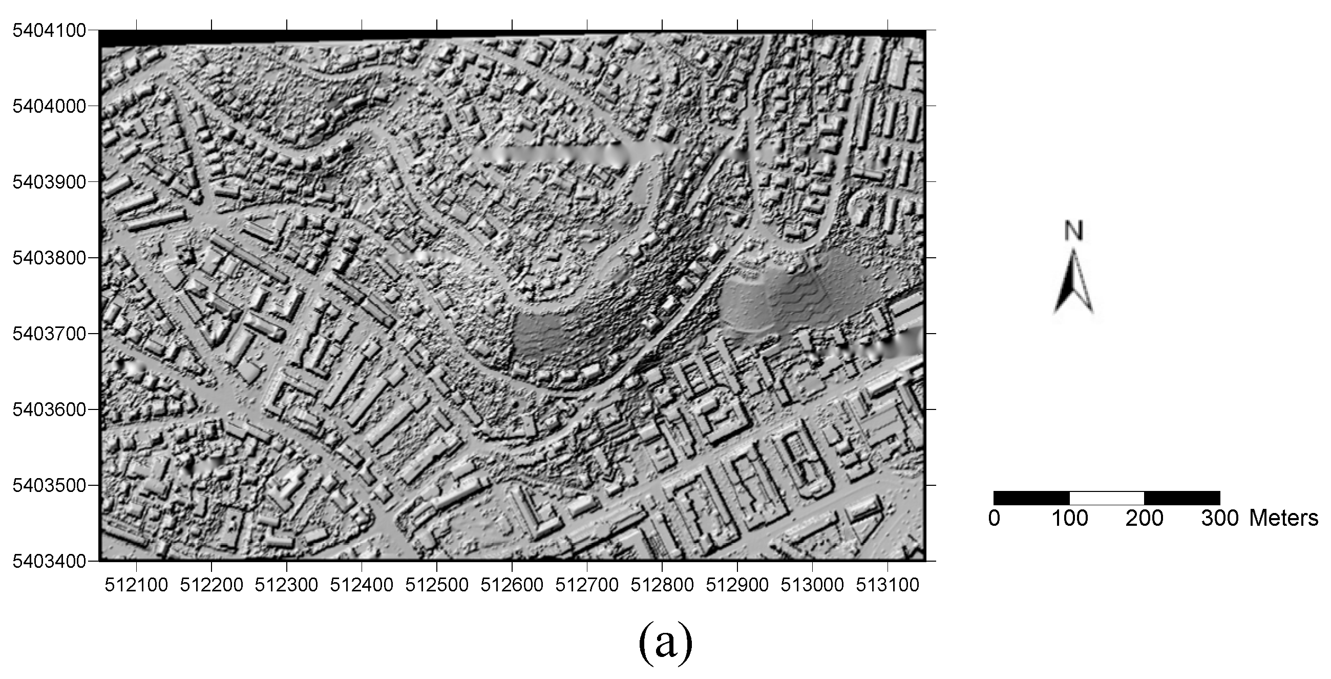
Steep terrain and complex objects are the biggest challenges for filtering.
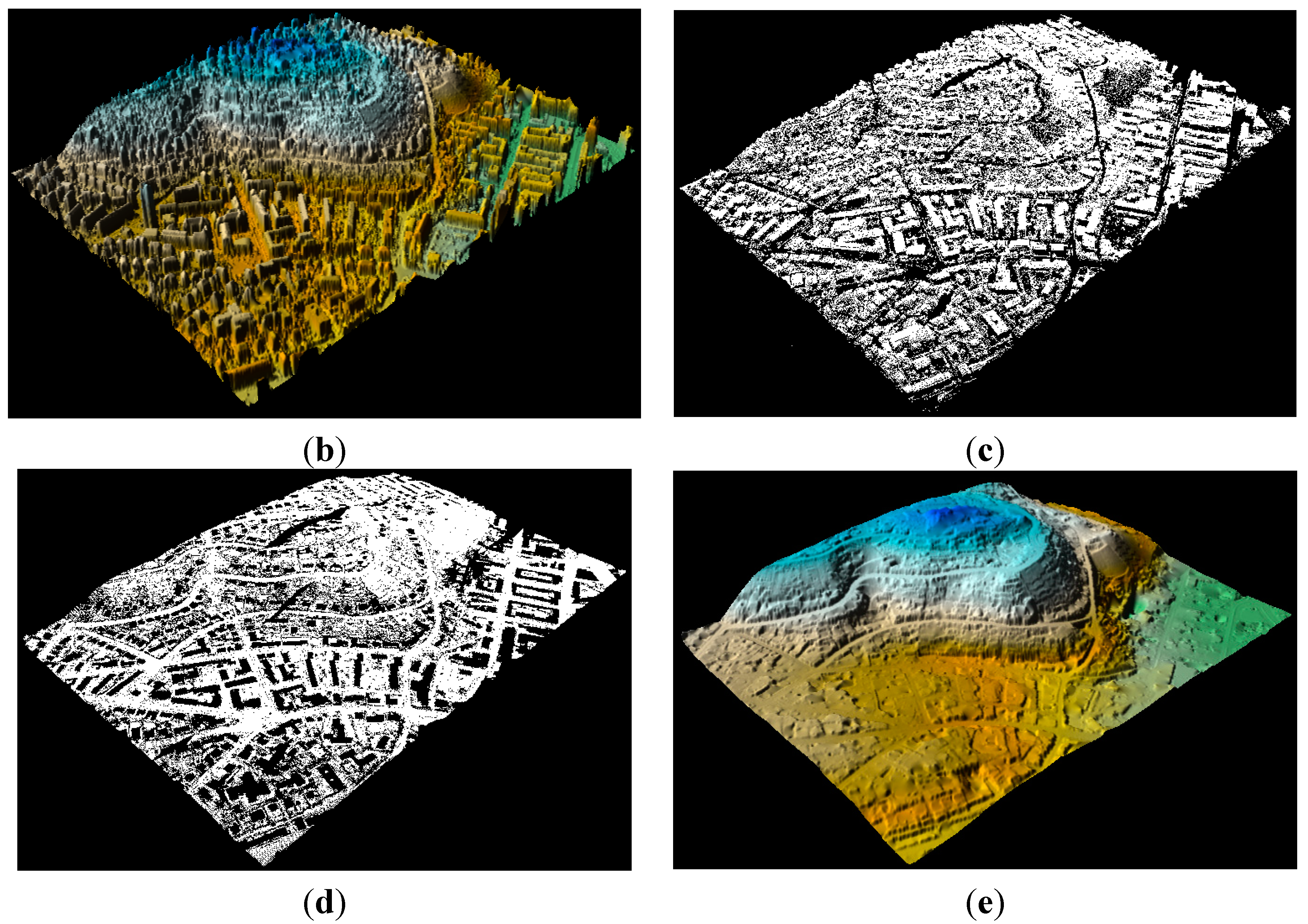
Figure 4a,b shows the digital surface model (DSM) generated from the raw point cloud of Site 1. A mixture of various buildings and vegetation on a rugged hillside, which are difficult to differentiate, clearly exists in the area.
Figure 4c,d show the nonground and ground points separated using the proposed filter. Both the distinct tall buildings and the lower surrounding objects are effectively distinguished. The main terrain relief features are well preserved, as shown by the comparison between the DSM in
Figure 4b and the digital elevation model (DEM) in
Figure 4e.
Figure 4.
Filtering results of the proposed method for the test data of Site 1: (a) DSM generated from the raw point cloud; (b) three-dimensional view of the DSM; (c) nonground points extracted by filtering; (d) ground points extracted by filtering; (e) DEM generated from the ground points.
Figure 4.
Filtering results of the proposed method for the test data of Site 1: (a) DSM generated from the raw point cloud; (b) three-dimensional view of the DSM; (c) nonground points extracted by filtering; (d) ground points extracted by filtering; (e) DEM generated from the ground points.
The results obtained by the proposed filter were compared with those obtained in the semiautomatic commercial software
Terrasolid TerraScan and other typical filtering methods [
10,
41] to quantitatively assess the proposed filter. Type I error, also called omission error, refers to the percentage of ground points misclassified as others. Type II error, also called commission error, refers to the percentage of object points misclassified as ground. Total error indicates the percentage of points misclassified in all points.
TerraScan is a widely used commercial software for processing lidar data.
Table 2 shows the results of
TerraScan filtering in the studied area as provided in [
31]. The proposed method produced smaller type I and total errors and slightly bigger type II error compared with the commercial software.
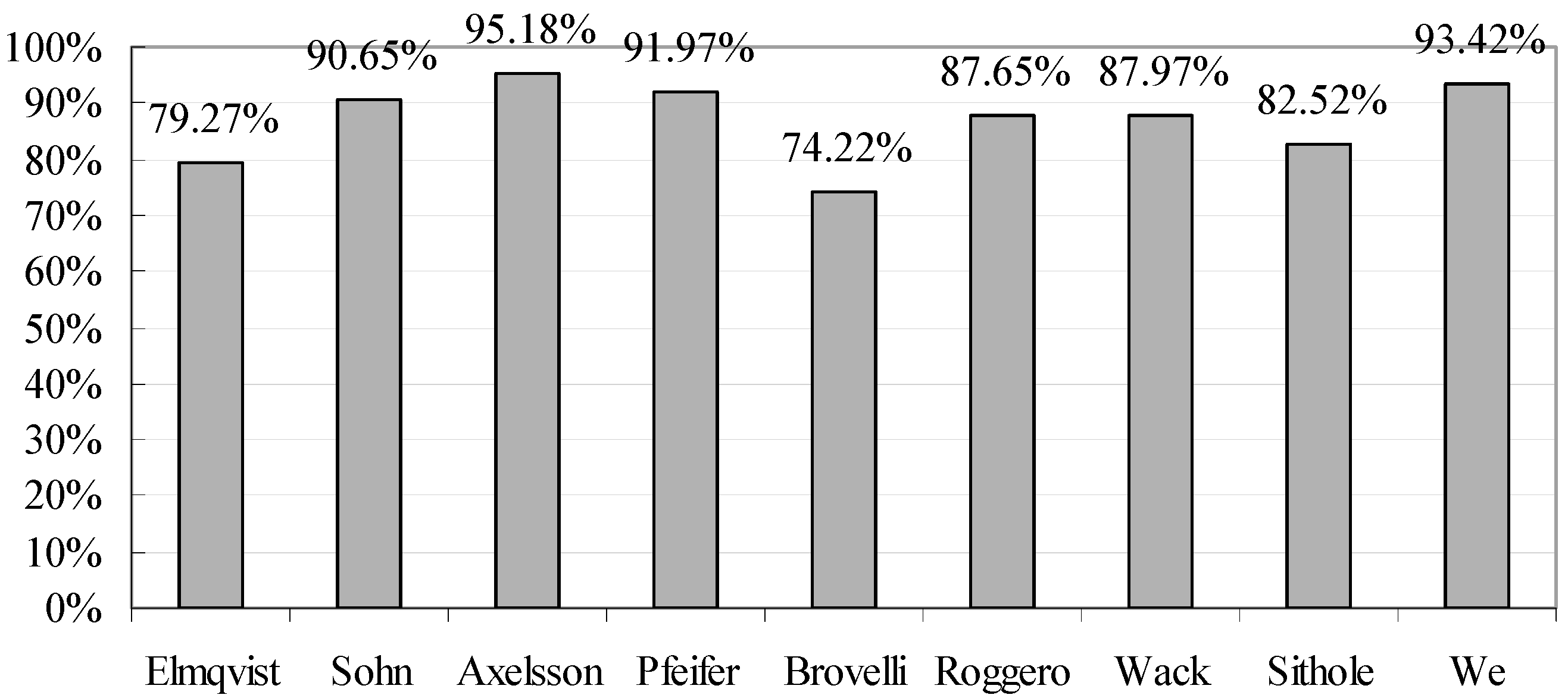
Figure 5 shows the comparison of the average overall accuracy of the proposed filter and that of eight different filtering methods tested by the ISPRS [
10]. Four methods with an average overall accuracy of more than 90% were identified for further comparison (see
Figure 6,
Figure 7,
Figure 8 and
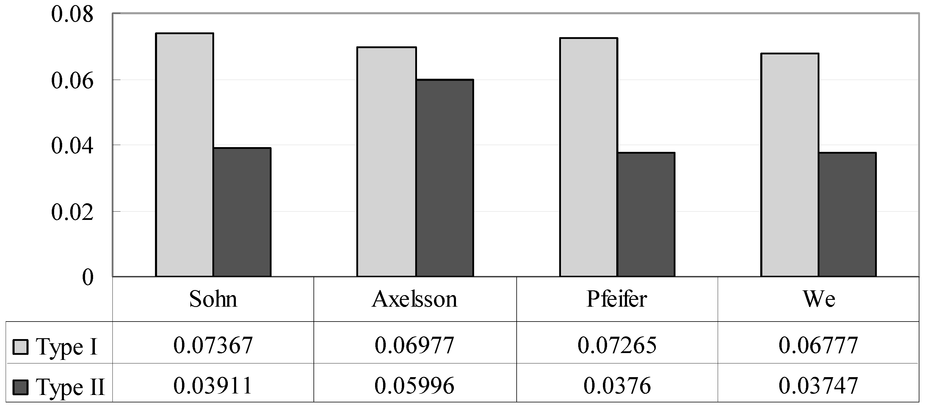
Figure 9). The comparisons of the results of the different filters demonstrate that the proposed filter has promising and competitive performance for various environments. Compared with the other two filters, the proposed method and that by Axelsson can both suppress omission and commission errors simultaneously at a minimal level.
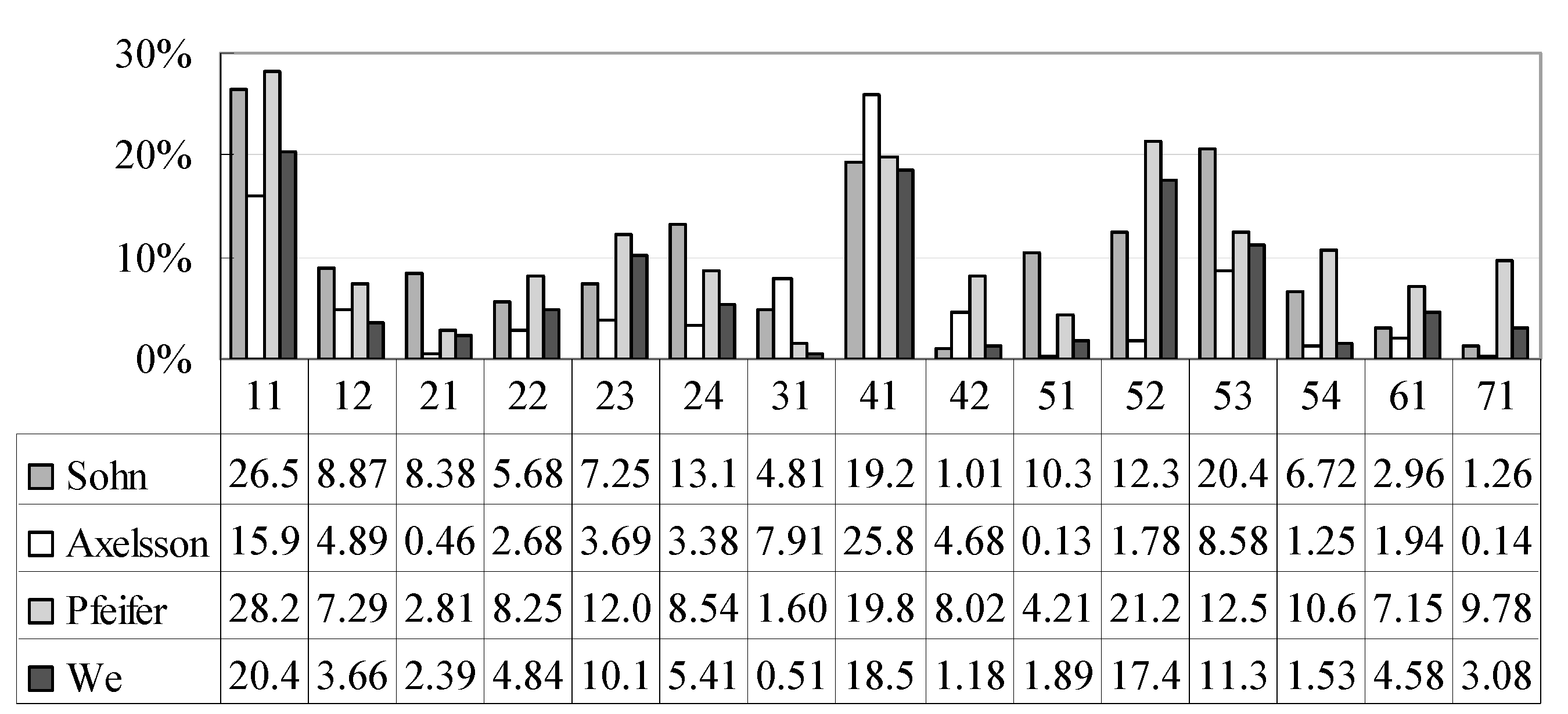
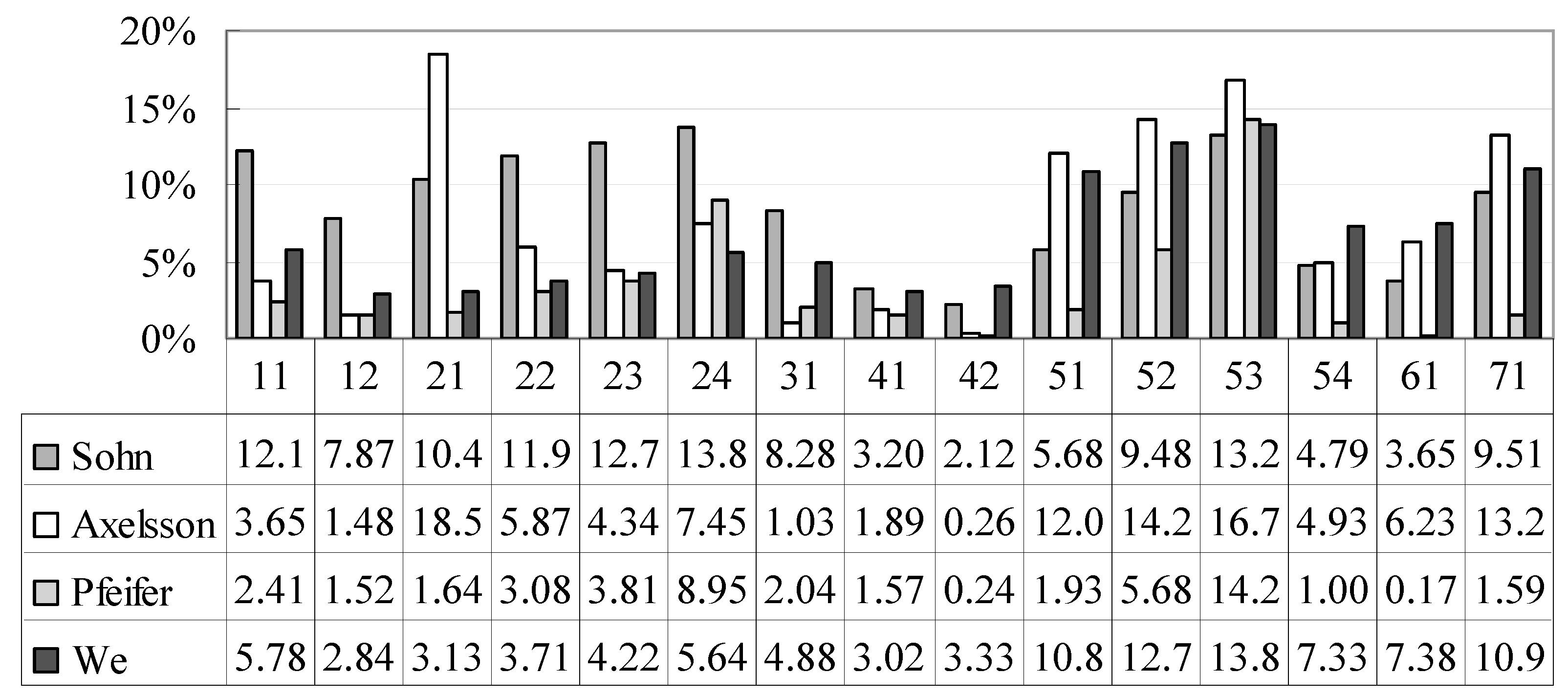
Figure 6,
Figure 7 and
Figure 8 show that Axelsson’s filter is biased toward type II errors, whereas our filter is oriented toward maintaining a balance between the two categories of errors. Moreover, Axelsson’s filter is incapable of distinguishing bridges from the ground [
8,
41], while our filter can remove bridges effectively, as shown in
Figure 10 and
Figure 11.
Figure 9 shows that our filter has minimal omission and commission error oscillation for different areas, thus confirming the stable and reliable performance of the proposed filter for diverse landscapes.
Table 2.
Comparison of errors of the proposed filter and TerraScan in filtering the ISPRS sample datasets.
Table 2.
Comparison of errors of the proposed filter and TerraScan in filtering the ISPRS sample datasets.
| Sample Dataset | TerraScan | Proposed Filter |
|---|
| Type I Error (%) | Type II Error (%) | Total Error (%) | Type I Error (%) | Type II Error (%) | Total Error (%) |
|---|
| 11 | 26.66 | 2.00 | 16.14 | 20.43 | 5.78 | 14.18 |
| 12 | 21.49 | 1.12 | 11.55 | 3.66 | 2.84 | 3.26 |
| 21 | 14.30 | 1.95 | 11.56 | 2.39 | 3.13 | 2.55 |
| 22 | 14.51 | 2.56 | 10.78 | 4.84 | 3.71 | 4.49 |
| 23 | 12.92 | 2.54 | 8.01 | 10.13 | 4.22 | 7.33 |
| 24 | 16.38 | 3.98 | 12.97 | 5.41 | 5.64 | 5.47 |
| 31 | 8.36 | 8.97 | 4.85 | 0.51 | 4.88 | 2.52 |
| 41 | 25.10 | 0.74 | 13.15 | 18.51 | 3.02 | 10.75 |
| 42 | 8.00 | 1.39 | 2.55 | 1.18 | 3.33 | 2.70 |
| 51 | 0.41 | 0.29 | 1.31 | 1.89 | 10.81 | 3.84 |
| 52 | 4.72 | 4.52 | 5.38 | 17.46 | 12.79 | 16.97 |
| 53 | 3.62 | 11.01 | 4.02 | 11.31 | 13.82 | 11.41 |
| 54 | 2.49 | 13.68 | 2.30 | 1.53 | 7.33 | 4.65 |
| 61 | 1.60 | 4.81 | 1.71 | 4.58 | 7.38 | 4.68 |
| 71 | 1.69 | 3.56 | 1.90 | 3.08 | 10.96 | 3.98 |
| Average | 10.82 | 3.75 | 7.20 | 7.13 | 6.64 | 6.58 |
Figure 5.
Comparison of the average overall accuracy of the different filtering algorithms used in the sample datasets.
Figure 5.
Comparison of the average overall accuracy of the different filtering algorithms used in the sample datasets.
Figure 6.
Comparison of type I errors in the filtered sample datasets.
Figure 6.
Comparison of type I errors in the filtered sample datasets.
Figure 7.
Comparison of type II errors in the filtered sample datasets.
Figure 7.
Comparison of type II errors in the filtered sample datasets.
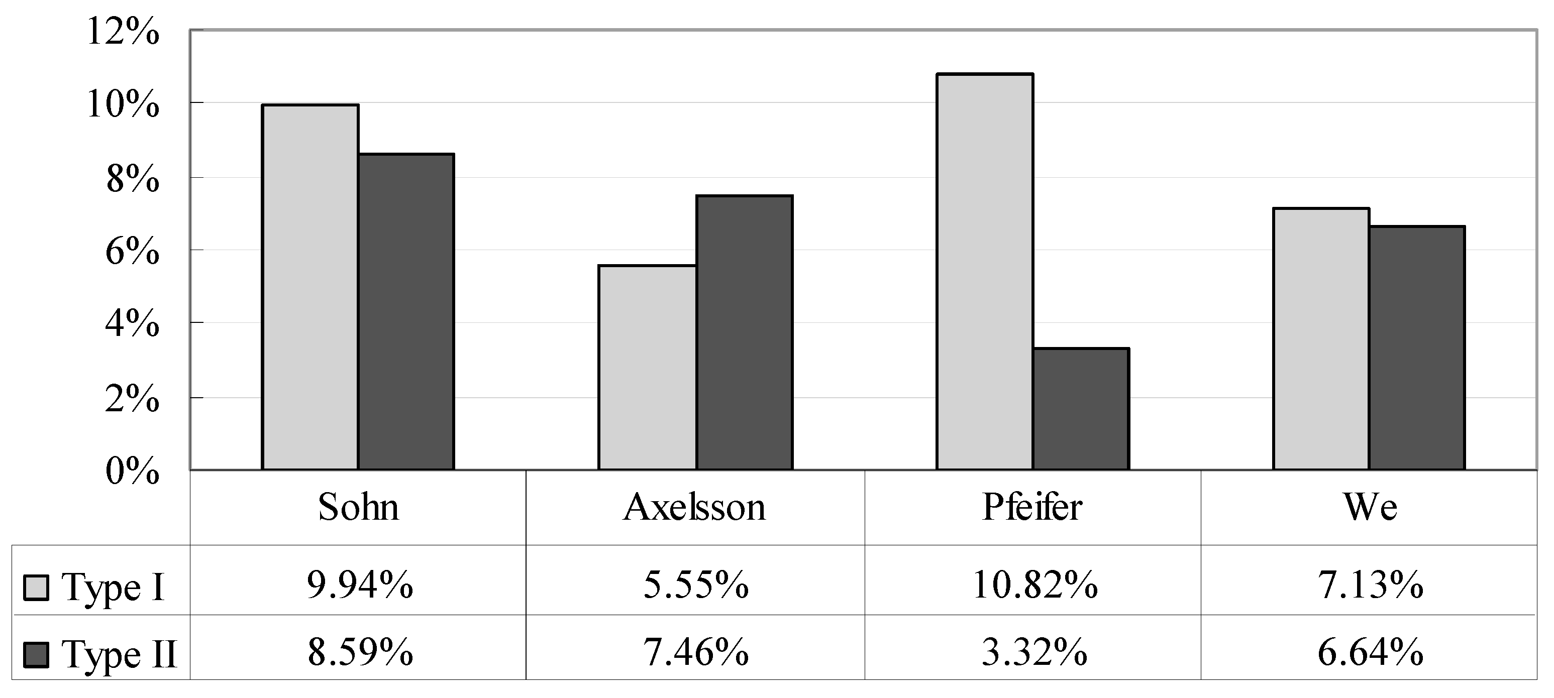
Figure 8.
Averages of type I errors and type II errors produced by different filters.
Figure 8.
Averages of type I errors and type II errors produced by different filters.
Figure 9.
Standard deviations of errors produced by different filters.
Figure 9.
Standard deviations of errors produced by different filters.
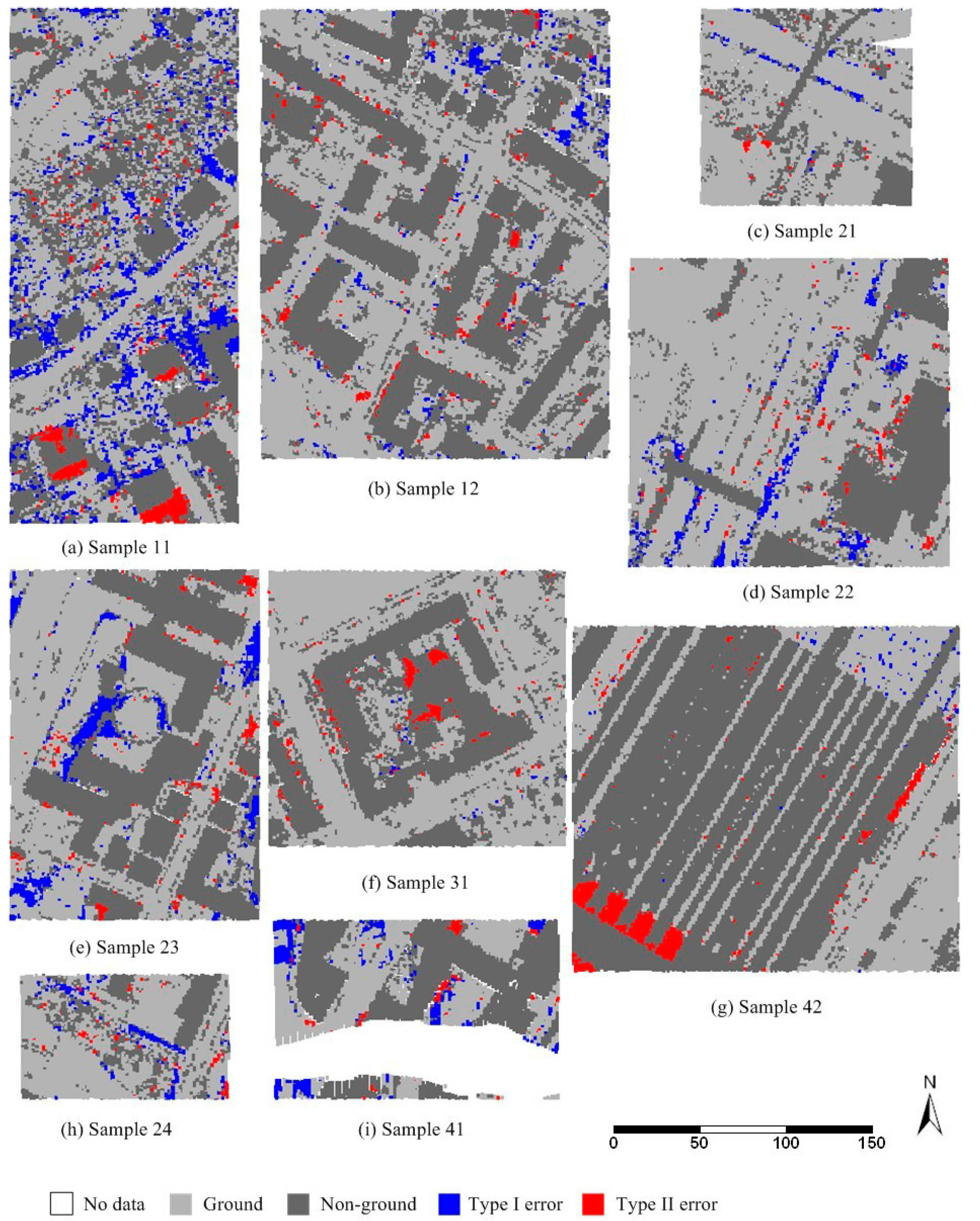
Figure 10.
Spatial distribution of errors generated by filtering urban sample datasets.
Figure 10.
Spatial distribution of errors generated by filtering urban sample datasets.
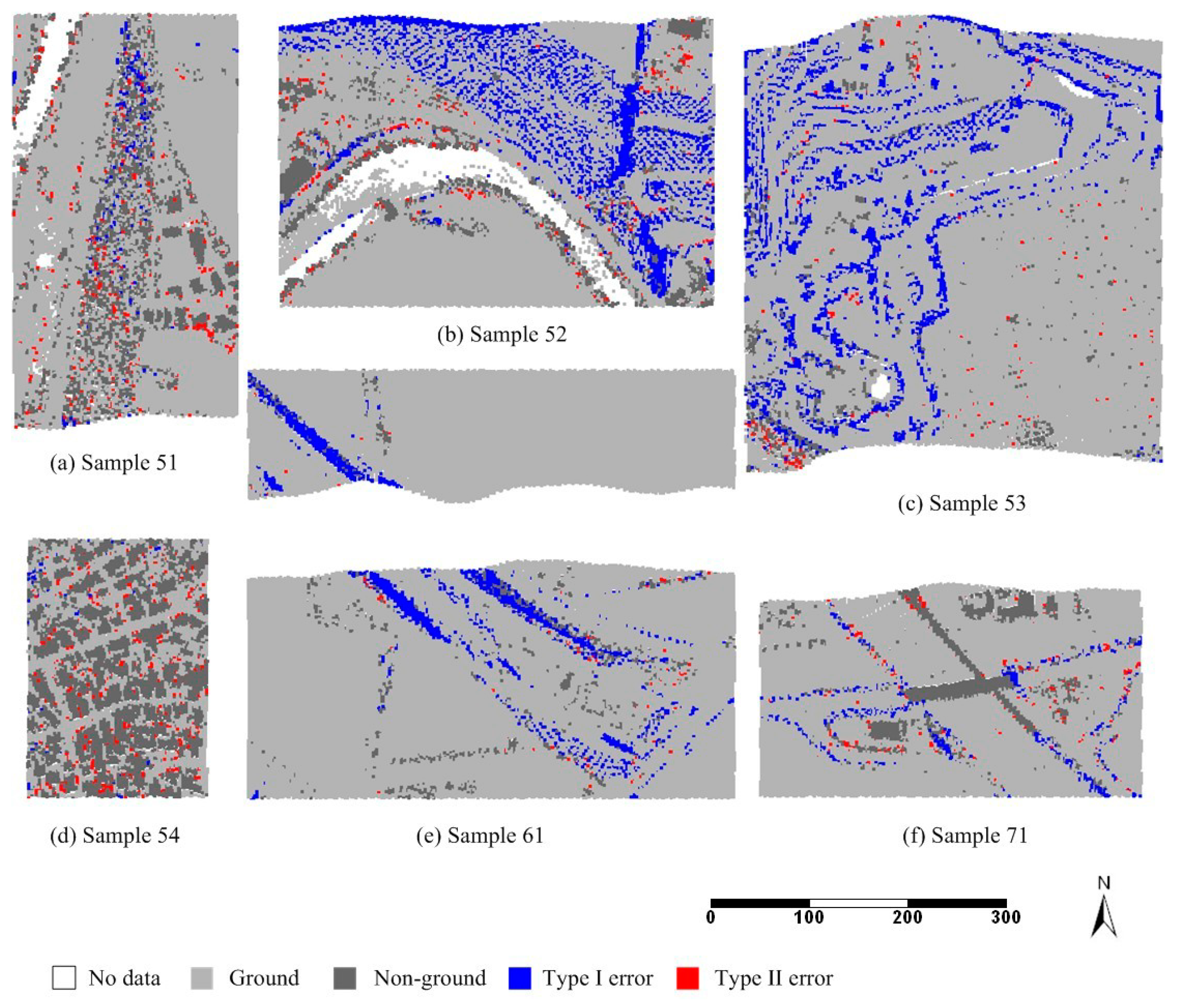
Figure 11.
Spatial distribution of errors generated by filtering rural sample datasets.
Figure 11.
Spatial distribution of errors generated by filtering rural sample datasets.
Figure 10 and
Figure 11 reveal the distribution of misclassified points across 15 samples filtered by the proposed algorithm, and
Table 3 and
Table 4 show the DSMs, true DEMs, and DEMs derived by filtering. The proposed filter further analyzes the top hats obtained by the brim filter extending outward to improve the traditional top-hat transformation. Adding a brim to the top hats is conducive to the analysis of different characteristics of objects and ground points, especially complex objects and abrupt terrains. The omission error generated by protruding terrain features is suppressed by the elevation change intensity of the transitions between the obtained top hats and the outer brims. Samples 22, 23, 51, 52, and 53 show various terrain features with dramatic elevation changes that were well preserved. The minute objects (e.g., vehicles and shrubs) were distinguished successfully using the minimum window size and height difference threshold (see sample 12). The diverse sizes and shapes of the objects in various environments did not have a significant effect on the filtration of samples 12, 22, 23, 31, and 41. The irregularly shaped buildings were mostly composed of multiple layers with various heights, which were effectively identified (see samples 22, 23, and 31). The result demonstrates the feasibility of verifying the nonground objects of complex structures using the sloped brim filter extending outwards. For filtering buildings and vegetation on steeply sloped hillside, various buildings and vegetation were effectively extracted while the main terrain features were well maintained (see samples 11, 24, 51, and 52). Terrain discontinuity was well preserved when filtering in rugged areas with dramatic elevation changes (see sample 53). The attached objects (e.g., bridges) were successfully removed (see samples 21, 22, and 71). Given that the morphological operations considered the local point sets covered by the window, the data gaps generated by scan swath or water absorption did not significantly influence the filter (samples 41, 51, 52, and 61). The iteration process in
Section 2 was carried out by assuming that the heights of the aboveground objects of a certain size were larger than one expected threshold and that the threshold increased as the object size increased. However, few low, large objects did not depict the common proportional relation of window size and height difference threshold defined by empirical formula (9). This condition led to the occurrence of commission errors (samples 11 and 42). Although the main terrain features were still maintained on the abrupt terrains, some ground points with dramatic height changes were rejected (samples 52, 53, and 61).
Table 3.
DSMs generated from the raw point clouds, DEMs generated from the true ground points, and DEMs generated from the ground points derived by the proposed filter for urban sample datasets.
Table 4.
DSMs generated from the raw point clouds, DEMs generated from the true ground points, and DEMs generated from the ground points derived by the proposed filter for rural sample datasets.
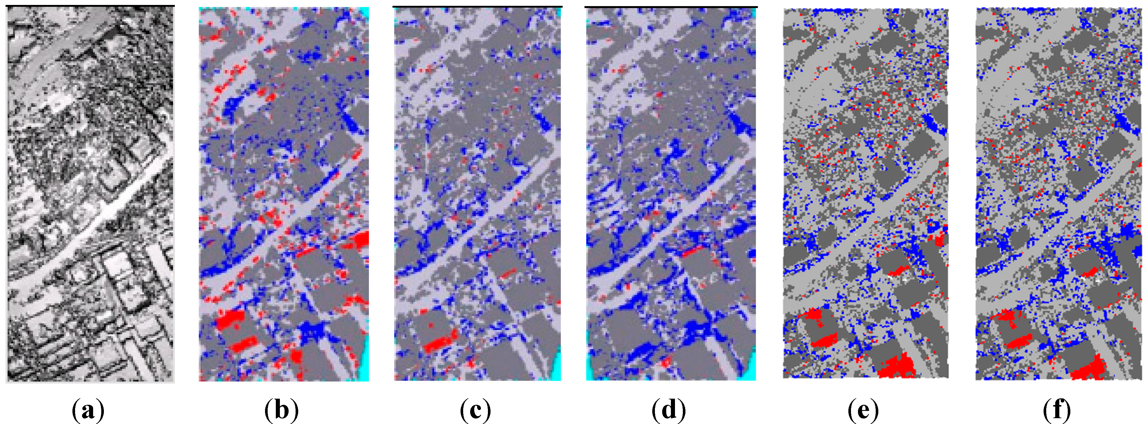
Figure 12,
Figure 13 and
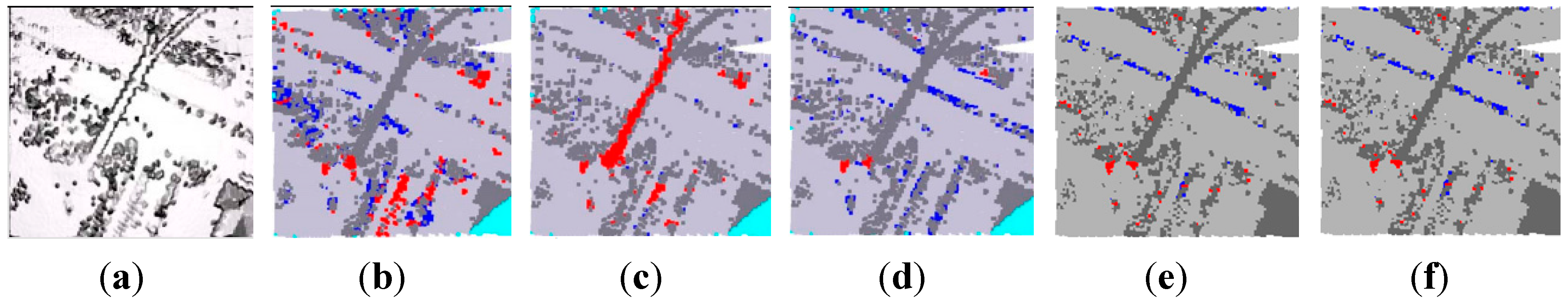
Figure 14 show the comparison of the filtering results of different filters for samples 11, 21, and 24. Vegetation and buildings on steep slopes are very challenging to distinguish, as in sample 11. Some ground points on very steep slopes were filtered off by those filters. The Sohn filter had heavy bias towards type II errors, while the Pfeifer had heavy bias towards type I errors. The proposed filter in this paper produced more type II errors than the Axelsson filter but less than the filter in [
38]. The produced type II errors were mainly at the bottom where laddered buildings occurred. The laddered buildings lie on steep slopes and have some parts with large size near to the slopes, which caused the morphological opening to make commission errors. As shown in
Figure 13, the centered bridge was not filtered in the Axelsson filter, while other filters including the proposed one could remove the bridge successfully. Ramps are a kind of structure spanning the gaps of discontinuous terrain surfaces with one side lower than the other, as centered in
Figure 14. Ramps were regarded as ground in [
41]. However, all the filters cut off the ramp in sample 24 because it was higher than the surface below.
Figure 12.
Comparison of the filtering results of different methods for sample 11: (
a) DSM generated from the raw point clouds; (
b) Sohn; (
c) Axelsson; (
d) Pfeifer; (
e) Li
et al. [
38]; (
f) This paper.
Figure 12.
Comparison of the filtering results of different methods for sample 11: (
a) DSM generated from the raw point clouds; (
b) Sohn; (
c) Axelsson; (
d) Pfeifer; (
e) Li
et al. [
38]; (
f) This paper.
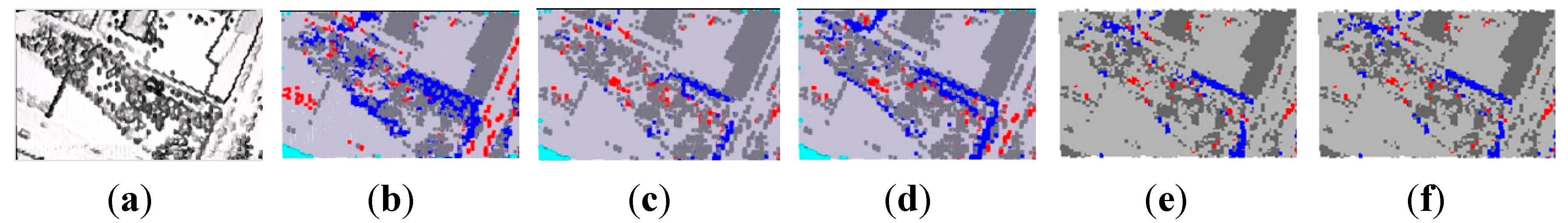
Figure 13.
Comparison of the filtering results of different methods for sample 21: (
a) DSM generated from the raw point clouds; (
b) Sohn; (
c) Axelsson; (
d) Pfeifer; (
e) Li
et al. [
38]; (
f) This paper.
Figure 13.
Comparison of the filtering results of different methods for sample 21: (
a) DSM generated from the raw point clouds; (
b) Sohn; (
c) Axelsson; (
d) Pfeifer; (
e) Li
et al. [
38]; (
f) This paper.
Figure 14.
Comparison of the filtering results of different methods for sample 24: (
a) DSM generated from the raw point clouds; (
b) Sohn; (
c) Axelsson; (
d) Pfeifer; (
e) Li
et al. [
38]; (
f) This paper.
Figure 14.
Comparison of the filtering results of different methods for sample 24: (
a) DSM generated from the raw point clouds; (
b) Sohn; (
c) Axelsson; (
d) Pfeifer; (
e) Li
et al. [
38]; (
f) This paper.
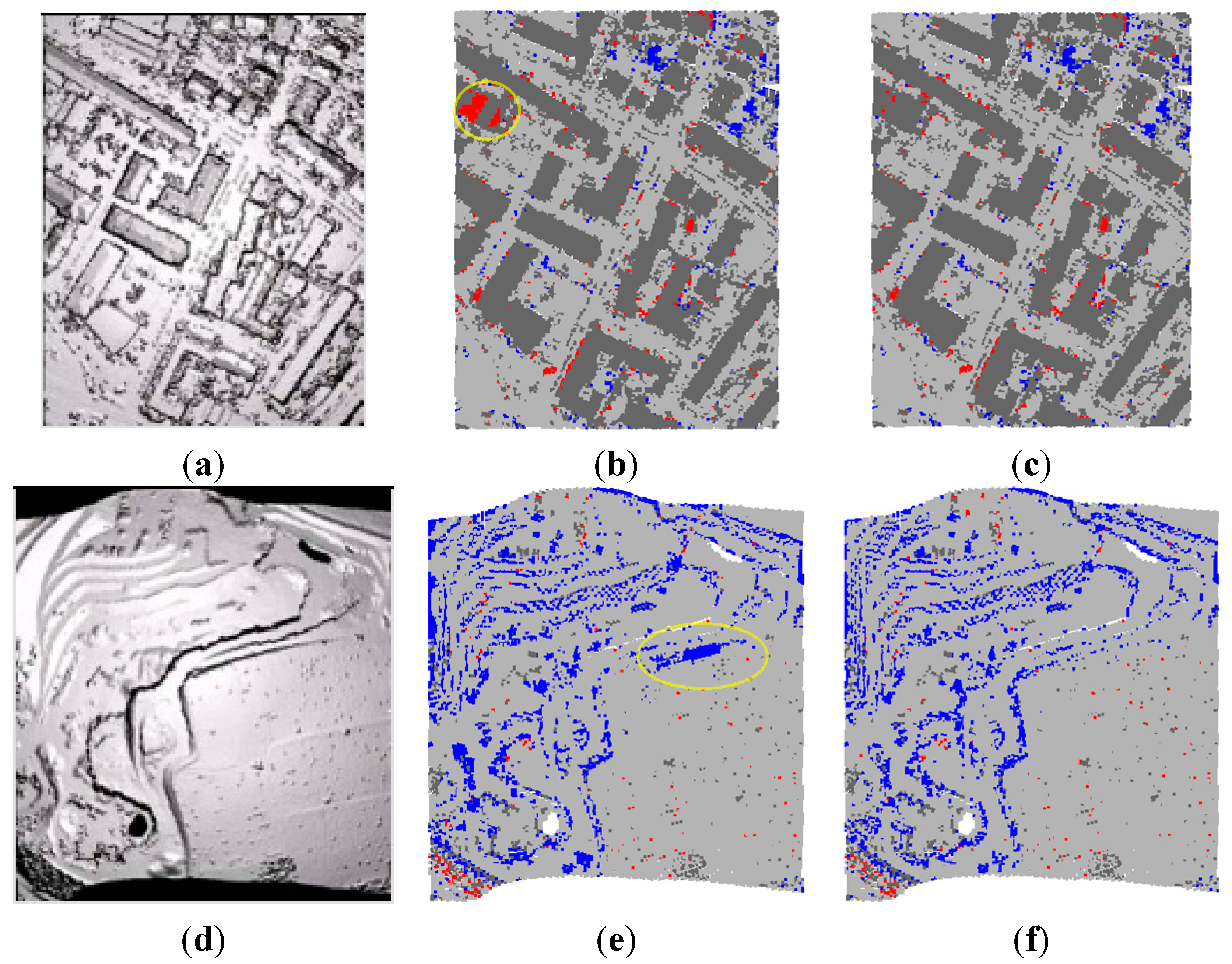
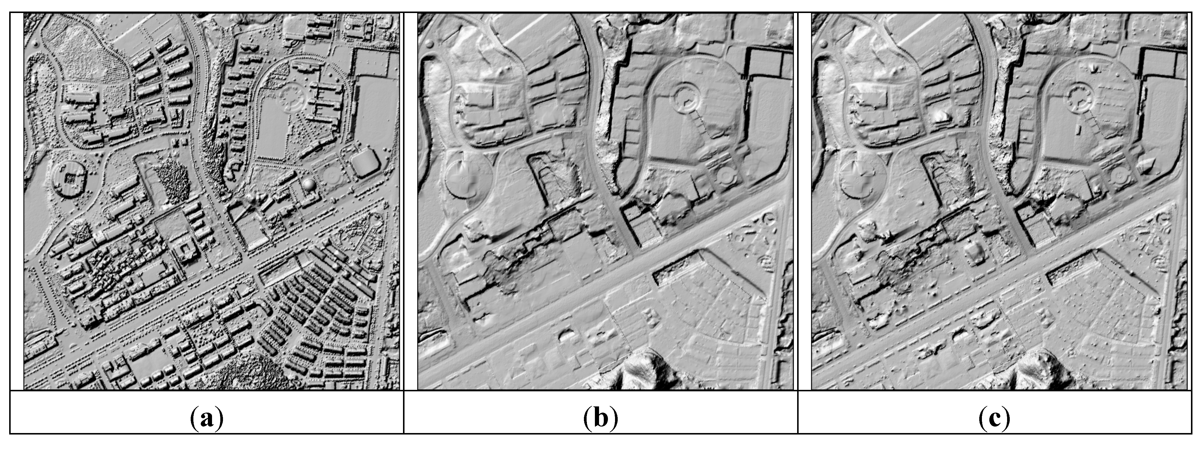
Although the filters proposed by Li
et al. [
38] and this paper are both based on mathematical morphology, the strategies and performances of the two filters are different. Nonground objects usually appear around the feature points with dramatic height changes, so Li
et al. [
38] focused on the redefinition of morphological openings to limit the filtered areas. The morphological erosion and dilation were only performed on the nearby points of the feature points, which could reduce the possibility of cutting the smooth terrain with a gradual height change. Afterwards a region growing approach was used to recall the removed points that were attached to other ground points. However, the filter in [
38] did not make special compensation for complex buildings with multilayer such as the one in the yellow circle in
Figure 15b, and thus the complex building parts were not eliminated. The proposed filter in this paper specially utilized the brim filter extending outward to increase the robustness for multilayer buildings, and thus the buildings were effectively distinguished, as shown in 15c. Although Li
et al. [
38] could suppress the omission errors to some extent, some discontinuous terrain features with abrupt height changes were missed as shown in the yellow circle in
Figure 15e. The proposed filter in this paper inspected the elevation change intensity of the transitions between the obtained top hats and outer brims to suppress the omission error caused by protruding terrain features, and thus it had a greater ability to preserve the distinctive terrain features in comparison to the filter in [
38], as shown in
Figure 15f. Moreover, the filter in [
38] was relatively time consuming due to the high requirement for neighboring searches and computation. Using Microsoft Visual C++ 6.0 IDE on a computer with 2.3 GHz Intel i3-2350 Processor and 2 GB RAM, the filter in [
38] spent 510.140 s to filter 683,204 points, while the proposed filter in this paper took 69.234 s due to its simple and efficient data structure and implementation such as executing brim filtering based on directional scanning on the index grid.
Besides the above mentioned filters,
Table 5 shows the three types of average errors of other recent algorithms performed in automatic mode against ISPRS samples. Chen
et al. [
33] improved upon morphological operations by adding a condition considering the elevation changes of the edge pixels of large features, which only reported the total errors. Jahromi
et al. [
42] filtered four urban study sites (samples 11, 12, 21, and 31) based on artificial neural networks. Susaki [
43] developed an adaptive slope filtering method to deal with the urban datasets (samples 11, 12, 21, 22, 23, 24, 31, 41, and 42). Zhang and Lin [
8] employed a point cloud segmentation using smoothness constraint to improve the progressive TIN densification for filtering all samples. The hierarchical surface interpolation used by Mongus and Zalik [
31] produced a larger commission error than omission error. Jahromi
et al. [
42] and Zhang and Lin [
8] have bias towards type I errors, while Susaki [
43] and Mongus and Zalik [
31] have bias towards type II errors. Minimizing type I errors contributes to reducing the total error because there are relatively more ground points than nonground points in most landscapes [
41]. Which error is the priority to suppress depends on the practical need in various applications. As shown by the comparison in
Table 5, the filter proposed in this paper keeps a balance between the commission error and omission error.
Figure 15.
Comparison of the filtering results of the methods proposed by Li
et al. [
38] and this paper for Samples 12 and 53: (
a) and (
d) are the DSMs generated from the raw point clouds; (
b) and (
e) are the results from Li
et al. [
38]; (
c) and (
f) are the results from the filter proposed in this paper.
Table 5.
Three types of average errors of recent automatic filters against ISPRS samples.
Table 5.
Three types of average errors of recent automatic filters against ISPRS samples.
| Author | Type I error (%) | Type II error (%) | Total error (%) |
|---|
| Chen et al. [33] | | | 7.22 |
| Jahromi et al. [42] | 11.00 | 3.47 | 7.70 |
| Susaki [43] | 6.70 | 11.26 | 7.39 |
| Mongus and Zalik [31] | 3.49 | 9.39 | 5.62 |
| Zhang and Lin [8] | 13.11 | 10.19 | 10.63 |
| This paper | 7.13 | 6.64 | 6.58 |
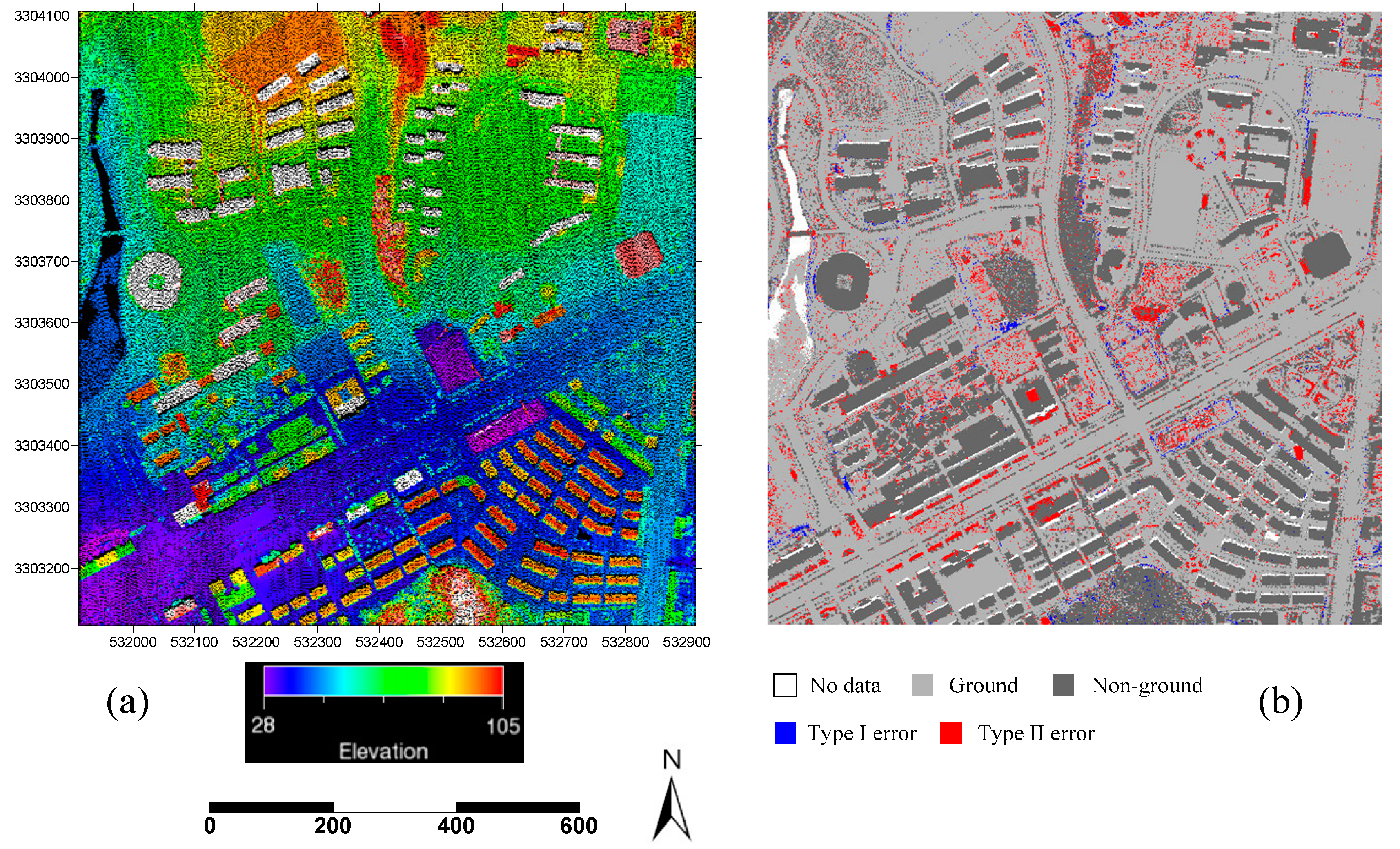
The proposed filter was applied to another dataset used in practice to test its performance under varying conditions in broad areas (
Figure 16 and
Figure 17). This dataset was acquired using the scanner Leica ALS50-II covering a 1 sq. km area in Xianning, China. The dataset included diverse objects and terrains suitable for assessing the performance of the proposed filter in complicated landscapes, such as many buildings with complex structures and shapes, dense vegetation, abrupt sloped terrains, and discontinuities in terrain, rivers, and bridges. Reference data were obtained by manual classification for accuracy evaluation. The number of points was 1,345,889 with an average point density of 1.35 points/m
2. The grid cell size of constructing spatial index was set to 1.4 m × 1.4 m for the data according to the point density.
Figure 16b shows the error distribution of the application of the filter to the data on Xianning City.
Figure 17 shows the DSM derived by raw point cloud and the DEMs derived from the reference data and filtered ground points. As shown in
Figure 16 and
Figure 17, the varied terrain features, especially the steep slopes and terrain discontinuities, were well preserved. Dense vegetation and complex buildings were effectively differentiated. Type I, type II, and total errors were 1.20%, 13.95%, and 6.02%, respectively. Type II error was mainly caused by very low objects, such as flower beds and grasslands, which widely exist in the study area. These very low objects are not in accordance with the relation between the height difference thresholds and window sizes defined by Equations (8) and (9). Hence, the morphological top-hat transformation did not remove them.
For the filter based on top-hat transformation, whether the filtering result is towards type I error or type II error mainly depends on the definition of the window size and the height difference threshold used in the iterative top-hat transformations. Using a large window and a small height difference threshold allows filtering to remove more objects, and meanwhile increases the possibility of cut terrain relief. Using a small window and a large height difference threshold allows filtering to keep terrain features intact, and meanwhile possibly prevents more objects from being filtered out. The practical surveyed areas usually cover various landscapes. In order to enhance the accuracy of filtering, we should utilize a large window and a small height difference threshold in even areas, and utilize a small window and a large height difference threshold in abrupt sloped terrains. So, how to automatically tune the window size and the height difference threshold based on the self-adaptive analysis of the considered areas is a promising research area to further improve the robustness.
Figure 16.
(a) Raw point clouds rendered by elevation. (b) The spatial distribution display of errors generated by filtering the data of Xianning City.
Figure 16.
(a) Raw point clouds rendered by elevation. (b) The spatial distribution display of errors generated by filtering the data of Xianning City.
Figure 17.
(a) DSM generated from the raw point clouds of Xianning City; (b) DEM generated from the true ground points; (c) DEM generated from the ground points derived by the proposed filter.
Figure 17.
(a) DSM generated from the raw point clouds of Xianning City; (b) DEM generated from the true ground points; (c) DEM generated from the ground points derived by the proposed filter.


