Mapping and Modelling Spatial Variation in Soil Salinity in the Al Hassa Oasis Based on Remote Sensing Indicators and Regression Techniques

Abstract

Soil salinity is one of the most damaging environmental problems worldwide, especially in arid and semi-arid regions. An integrated approach using remote sensing in addition to various statistical methods has shown success for developing soil salinity prediction models. The aim of this study was to develop statistical regression models based on remotely sensed indicators to predict and map spatial variation in soil salinity in the Al Hassa oasis. Different spectral indices were calculated from original bands of IKONOS images. Statistical correlation between field measurements of Electrical Conductivity (EC), spectral indices and IKONOS original bands showed that the Salinity Index (SI) and red band (band 3) had the highest correlation with EC. Combining these two remotely sensed variables into one model yielded the best fit with R² = 0.65. The results revealed that the high performance of this combined model is attributed to: (i) the spatial resolution of the images; (ii) the great potential of the enhanced images, derived from SI, by enhancing and delineating the spatial variation of soil salinity; and (iii) the superiority of band 3 in retrieving soil salinity features and patterns, which was explained by the high reflectance of the smooth and bright surface crust and the low reflectance of the coarse dark puffy crust. Soil salinity maps generated using the selected model showed that strongly saline soils (>16 dS/m) with variable spatial distribution were the dominant class over the study area. The spatial variability of this class over the investigated areas was attributed to a variety factors, including soil factors, management related factors and climate factors. The results demonstrate that modelling and mapping spatial variation in soil salinity based on regression analysis and remote sensing data is a promising approach, as it facilitates timely detection with a low-cost procedure and allows decision makers to decide what necessary action should be taken in the early stages to prevent soil salinity from becoming prevalent, sustaining agricultural lands and natural ecosystems.

1. Introduction

Soil salinity refers to surface or near-surface accumulation of salts [1]. It is a worldwide environmental problem that mainly occurs in arid and semiarid regions and causes soil degradation [2]. The spatial variability of soil salinity over the landscape is highly sensitive and controlled by a variety factors. These factors include soil factors (parent material, permeability, water table depth, groundwater quality and topography), management factors (irrigation and drainage) and climatic factors (rainfall and humidity) [3]. The characterization of soil salinity is generally done measuring the electric conductivity (EC) in a saturated soil paste or in aqueous extracts with different soil/water ratios and using a spectrometer [4,5]. To elaborate detailed maps, density of soil samples using the previous technique is required, through an extensive design, which makes mapping time consuming and expensive.

In recent decades, there has been a widespread application of remote sensing data to map soil salinity, either directly from bare soil or indirectly from vegetation in a real-time and cost-effective manner at various scales [6]. Beside, assessing soil salinity spatial modelling, which is the utilization of numerical equations to simulate and predict real phenomena and processes, has followed several approaches. The approaches used range from artificial neural network [7–10], to classification and regression tree [11,12], to fuzzy logic [13], to generalized Bayesian analysis [14], to geostatistics (e.g., Kriging, CoKriging and regression kriging) [15–18] and statistical analysis (e.g., regression, ordinary least squares) [10,19–21]. An overview of these techniques and how they provide optimal results under certain circumstances is given in the review papers of McBratney et al. [22] and Scull et al. [23].

An integrated approach using RS in addition to various statistical methods has great potential for developing soil prediction models. In the case of soil salinity, statistical analysis, in particular linear regression, has created a tremendous potential among other techniques for improvement in the way that soil salinity is modelled, because of its rapid, practical and cost-effective manner [22,24]. A variety of statistical models based on remote sensing data has been developed and has revealed reasonable predictors of soil salinity in the literature [16,18,20,25–35]. In Thailand, Shrestha [27] developed several salinity prediction models containing spectral variables, including Normalized Difference Vegetation Index (NDVI), Normalized Difference Salinity Index (NDSI), the eight original bands of Landsat Enhanced Thematic Mapper plus (Landsat ETM+) and soil properties. The results indicated that mid-infrared (band 7) and near-infrared (band 4) had the highest association with the measured EC. Combining these variables yielded salinity prediction models to infer soil salinity over a large area. In contrast, Mehrjardi et al. [30] found that among the Landsat ETM+ bands 1–5 and 7, band 3 (red band) had the highest correlation with EC, and based on that result, a regression model fitted to relate EC to band 3 and the exponential relation was found to be the best type of model.

A regression model based on image enhancement techniques (spectral indices, Principal Components Analysis (PCA) and Tasseled Cap Transformation (TCT)) have also been extensively used to predict soil salinity and to improve the characterised variability of salinity. For example, Tajgardan et al. [36] combined Principal Components Analysis (PCA) techniques and regression analysis to predict and map soil salinity from data collected by the Advanced Spaceborne Thermal Emission and Reflection Radiometer (ASTER) at the north of the Aq-Qala Region in northern Iran. From this study, a suitable regression model was developed with electrical conductivity (EC) to predict and map soil salinity. Similarly, Afework [33] built a reliable model to predict soil salinity in the Metehara sugarcane farms in Ethiopia by relating EC to the Normalized Difference Salinity Index (NDSI) using linear regression.

Other researchers found that incorporating satellite images spectral bands with enhanced images has great promise for soil salinity modelling and mapping. Bouaziz et al. [37] conducted a study to detect soil salinity based on the Moderate Resolution Imaging Spectroradiometer (MODIS) and a multiple linear regression. They found that incorporating Salinity Index SI2 with near-infrared (NIR) (band 3) into a statistical model allowed researchers to gain great insight into the spatial detection of the spread of soil salinity. Recently, Judkins and Myint [20] found that Landsat band 7, Transformed Normalized Vegetation Index (TNDVI) and Tasselled Cap 3 and 5, derived from TCT, provided high correlation to the variation in soil salinity. Combining these spectral variables into a multiple linear regression model enabled them to predict and map soil salinity surface variation levels efficiently.

Most of the reviewed studies and others found in the literature modelled soil salinity using statistical analysis and multispectral images with moderate spatial resolution (e.g., Landsat, MODIS, etc.), while only in limited studies multispectral high spatial resolution images such as IKONOS, were used [19]. Moreover, several studies have been undertaken for mapping and modelling soil salinity over vegetation species other than date palms, and so far, a limited study has been undertaken to map soil salinity in a primarily date palm region. One such region is Al Hassa oasis in the eastern province of Saudi Arabia, which is the most productive date palm (Phoenix dactylifera) farming regions in Saudi Arabia and is seriously threatened by soil salinity. Although the date palm is highly tolerant of soil salinity, the growth and productivity of date palms in this oasis are being negatively impacted by an increasing soil salinity problem [38]. Thus, predicting the variability of soil salinity and mapping its spatial distribution are becoming increasingly important in order to implement or support effective soil reclamation programs that minimize or prevent future increases in soil salinity.

The overall aim of this study was to develop effective combined spectral-based statistical regression models using IKONOS high-resolution images to predict and map spatial variation in soil salinity in the Al Hassa oasis, a region dominated by date palms.

2. Materials and Methods

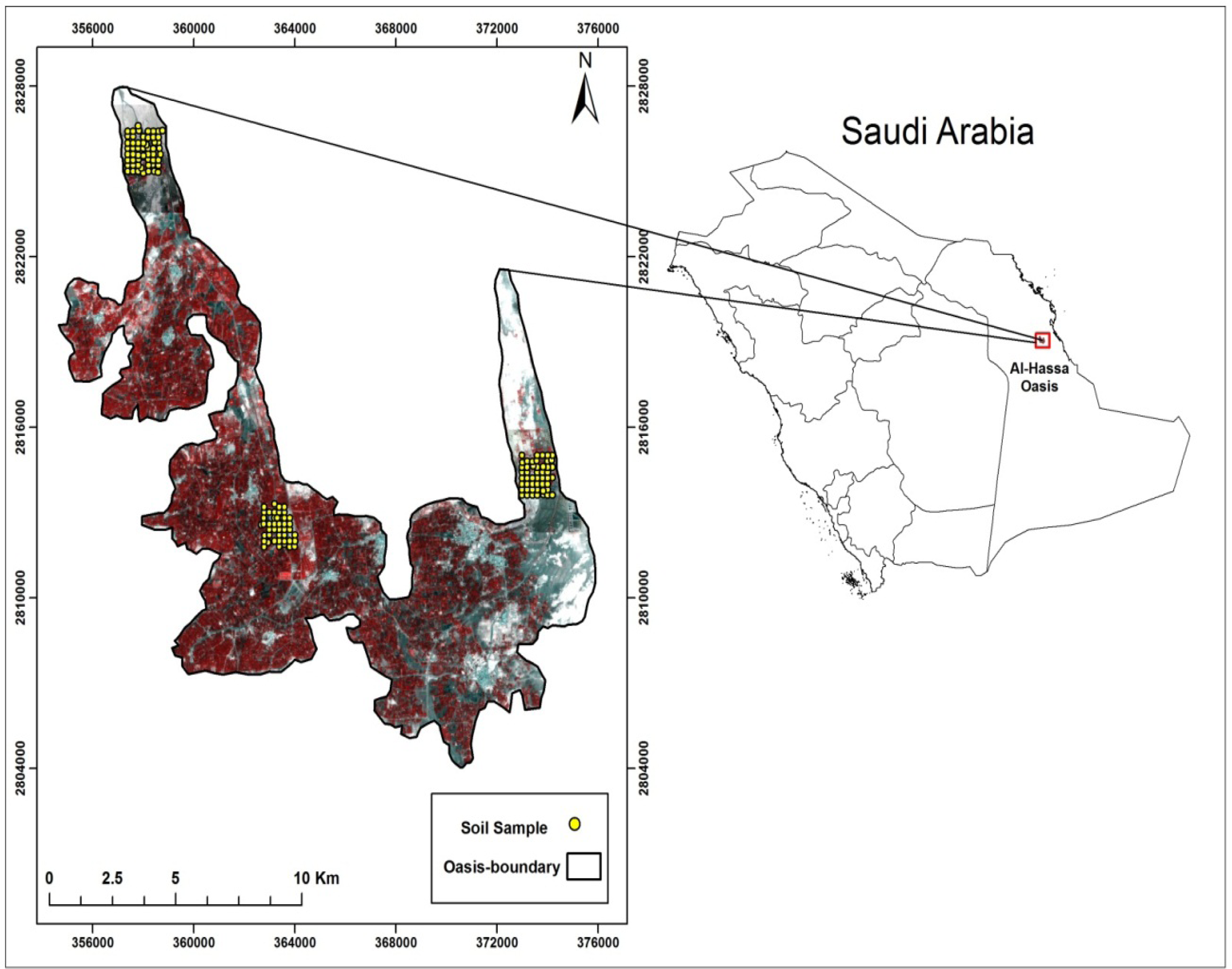
2.1. Study Area

The Al Hassa oasis is situated approximately 70 km inland of the gulf coast between a latitude of 25°05′ and 25°40′N and a longitude of 49°10′ and 49°55′E (Figure 1). This oasis covers an area of approximately 20,000 ha and is at an altitude of approximately 130 to 160 m above sea level [39,40]. The Al Hassa oasis is L-shaped and is actually composed of two separate oases [41]. The main water sources include the Neogene groundwater aquifer and some free flowing springs that are distributed across the area [42]. The oasis groundwater is primarily used for domestic, irrigation and industrial purposes. The oasis is characterized by an arid climate with a high potential evaporation rate that goes above the annual average precipitation of approximately 488 mm. The absolute ambient temperature exceeds 45 °C during the summer season (from June to August). During the winter (December to February), the temperature is between 2 and 22 °C. The study area covers six different soil types, which are Torripsamments, Torriorthents, Calciorthids, Salorthids, Gypsiorthids and Haplaquepts [43,44]. The particle size distribution reveals that soils are sandy loam in texture.

2.2. Field Sampling

Three sampling sites were selected based on the division of the oasis and different amounts of vegetation. The first site was located in the northern part of the oasis at Al-Uyoun city, which is characterised by low vegetation cover. The second site, in the middle of the oasis at Al-Bataliah village, had high vegetation cover. The last set of samples was collected under medium vegetation cover in the eastern oasis, which is located in the town of Al-Umran (Figure 1).

Composite soil sampling was performed during January and February (the dry season) of 2012 following the sampling procedures of Bouaziz et al. [45]. The exact coordinates of each composite sample were registered using a global positioning system (GPS) with an accuracy of ±5 m. Each composite soil sample was comprised of four core sub-samples that were collected at a distance of 20 m north, south, east and west of the centre sampling point. The sub-samples were collected from the surface horizon (0–20 cm) with a hand auger (10 cm diameter) and were crushed and mixed together to form one sample. A total of 149 composite soil samples were collected from the three defined sites. Soil salinity can be measured directly by measuring the EC in the field and remotely, including the lab measurement. However, since the aim of this study is to establish a relationship between EC and satellite spectral band and extrapolate point information to generate a soil salinity map of study area, soil salinity direct measurement was performed by measuring the EC in the soil saturation extracts in the laboratory, as described by Richards [46].

2.3. Satellite Data Acquisition and Processing

High spatial resolution cloud-free IKONOS satellite images were used in this study and were acquired near the actual soil sampling date on 20 April 2012. The IKONOS images include multispectral bands (blue, 0.40–0.52 μm; green, 0.52–0.60 μm; red, 0.63–0.69 μm; near-infrared (NIR), 0.76–0.90 μm) and record the reflected or emitted radiation from the Earth’s surface [47]. The images were geo-rectified to a Universal Transverse Mercator (UTM) coordinate system using World Geodetic System (WGS) 1984 datum assigned to north UTM zone 39. Atmospheric correction was performed using the Dark-Object Subtraction (DOS) technique [48]. All the remote sensing data processing was performed using the Environment for Visualizing Images (ENVI) version 4.8 software.

2.4. Data Analysis, Model Generation and Selection

Initially; the EC data was tested to establish whether it conformed to a normal distribution. The normality test exhibited that EC data had positive-skewed frequency distributions; thus, Box-Cox transformation was carried out to improve sample symmetry and to stabilise the spread. As part of the model generation process, various spectral soil salinity indices were tested for assessing and enhancing the variations in surface soil salinity. Out of all indices tested, the Salinity Index (SI) (Equation (1)), which has been proposed by Tripathi et al. [49], was used to create enhanced images for soil salinity in this study, due to its very highly significant correlation with EC. To ascertain the spatial location of the soil samples; a convolution low pass filter with a kernel size of 5 × 5 was applied to the enhanced images, then digital values were extracted at the location of sample points over those enhanced images.

$$\text{Salinity}\hspace{0.17em}\text{Index}\hspace{0.17em}(\text{SI})=\frac{\text{R}}{\text{NIR}}\times 100$$

(1)

where R is the red band and NIR is the near-infrared band of the IKONOS image.

Subsequently, Pearson Correlation analysis between the four bands (blue, green, red and near-infrared) and SI with EC were conducted to reveal the relationship between these variables and assess their efficiency in predicting soil salinity. The explanatory variables chosen were those showing the highest significant correlations with EC.

To build the regression model, samples were randomly split into two subsets. One subset was used for training (n = 98), the other for testing purposes (n = 51). Deciding which explanatory variables to include in the regression model is not always easy, and increasing the number of variables in a model may lead to an over-fit and provide poor prediction when used with a different data set [50]. To overcome these issues, stepwise regression was used to determine the variables that best explained most of the variability of the dependent variable, which was EC. Once all the developed regression models were tested, models with (i) a high R², signifying a strongly linear relationship, (ii) low standard errors of the model’s variables and (iii) few variables with a p-value of <0.05 were selected for evaluation using the testing data. Consequently, the best performed regression model that met all the model selection and validation criteria was chosen and used to predict and map the spatial variation in soil salinity. All statistical analyses were undertaken in JMP^®10 (JMP statistical discovery software from SAS), and significance levels set to p < 0.05.

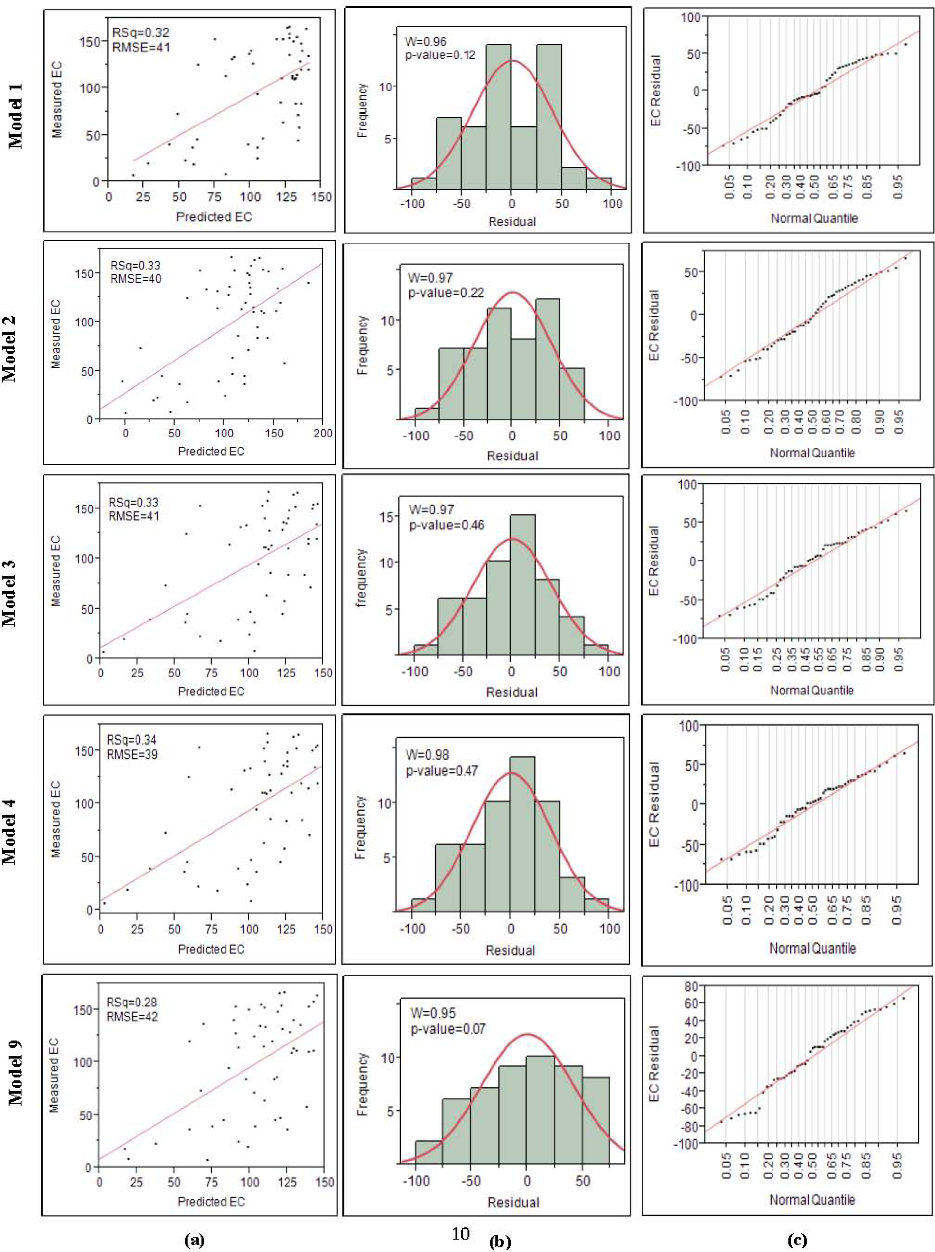
2.5. Model Validation

The performance of the developed regression models that met the model selection criteria was quantified using the testing subset to ensure that they not only worked on one particular data set but also yielded an accurate result on different data sets. Two quantitative criteria between measured and predicted values were calculated (

Table 1. Statistical criteria for evaluating the regression model.

Function Name	Equation	Equation Number
Coefficient of determination	$$R^2=(\frac{{\sum }_{i=1}^n\left({\chi }_i-\overline{\chi }\right)({\gamma }_i-\overline{\gamma })}{\sqrt{{\sum }_{i=1}^n{({\chi }_i-\overline{\chi })}^2+{\sum }_{i=1}^n{\left({\gamma }_i-\overline{\gamma }\right)}^2}})$$ (2)
Root mean square error	$$\mathit{RMSE}=\sqrt{\frac{{\sum }_{i=1}^n{\left({\chi }_i-{\gamma }_i\right)}^2}{n}}$$ (3)

^*χ_i and γ_i are measured and predicted values, respectively; χ̄ and γ̄ represent the means of the measured and predicted values, respectively; n is the number of samples.

). R² values indicate the strength of the statistical linear relationship between measured and predicted soil salinity values, and Root Mean Square Error (RMSE) indicates absolute estimation errors [51]. In addition to these criteria, histograms, normal probability plots and Shapiro–Wilk tests (W) were employed to assess whether or not the residuals present a normal distribution. If the W test is significant (p < 0.05) or highly significant (p < 0.001) then the distribution is non-normal [52].

3. Results

3.1. Data Analysis

The main statistical parameters for EC data are given in

Table 2. Descriptive statistics of electrical conductivity (EC).

	Mean	Max	Min	SD	CV (%)
EC	73.37	202	1.43	62.65	85.39

Max: maximum; Min: minimum; SD: standard deviation; CV: coefficient of variation.

. According to the soil salinity classification of the Food and Agriculture Organization (FAO), EC values of the study area vary from very strongly saline (>16 dS/m) to non-saline (0–2 dS/m). The high Co-efficient of Variation (CV) of 85.39% confirms the variations of the EC values over the study area. About 73% of the total samples were classified as very strongly saline soil, signifying that this is the dominant soil salinity class. Correlation analysis showed a significant positive correlation (p < 0.001) between EC and remotely sensed data of the blue (B1), green (B2), red (B3) and SI, respectively, but not with near-infrared (B4) (

Table 3. Correlation coefficient between EC and remotely sensed data.

Variables	B1	B2	B3	B4	SI
EC	0.41 ***	0.42 ***	0.45 ***	0.06 ns	0.70 ***

Significant:

^*p < 0.05;

^**p < 0.01;

^***p < 0.001; ns = not.

).

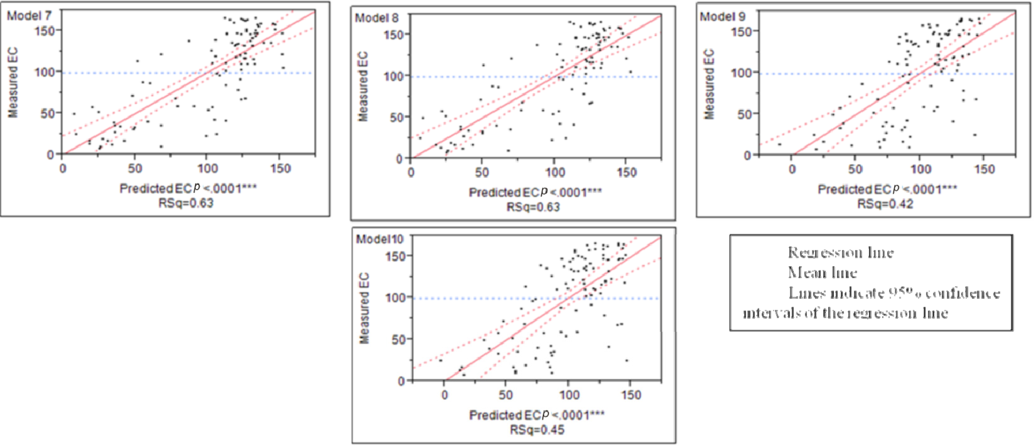
3.2. Models Development and Valuations

Remotely sensed data with a significant correlation to EC were considered for developing the regression models. The developed regression models are shown in Figure 2 and their statistical results are summarized in

Table 4. Developed regression models to predict EC based on remotely sensed data. SI, Salinity Index.

Model	Variable	Regression Coefficient	Standard Error	p-Value
1	Intercept	−239.49	29.82	<0.0001 ***
	SI	3.52	0.31	<0.0001 ***
	R = 0.76***, R2 = 0.58 ***
2	Intercept	−205.25	29.95	<0.0001 ***
	SI	−1.77	0.511	0.0008 ***
	B1	4.83	0.48	<0.0001 ***
	R = 0.79***, R2 = 0.62 ***
3	Intercept	−239.60	28.31	<0.0001 ***
	SI	4.83	0.48	<0.0001 ***
	B2	−1.011254	0.30	0.001 **
	R = 0.79***, R2 = 0.62***
4	Intercept	−269.13	29.99	<0.0001 ***
	SI	4.87	0.52	<0.0001 ***
	B3	−0.83	0.26	0.002 **
	R = 0.81***, R2 = 0.65***
5	Intercept	−193.18	83.48	0.02 *
	SI	4.81	0.49	<0.0001 ***
	B1	−2.39	4.04	0.5559
	B2	0.36	2.35	0.8771
	R = 0.79***, R2 = 0.62***
6	Intercept	−136.12	93.24	0.1476
	SI	4.64	0.54	<0.0001 ***
	B1	−3.59	2.38	0.1356
	B3	0.95	1.21	0.4355
	R = 0.79***, R2 = 0.63***
7	Intercept	−115.70	84.33	0.1734
	SI	4.31	0.59	<0.0001 ***
	B2	−4.97	2.56	0.0551
	B3	3.49	2.24	0.1226
	R = 0.79***, R2 = 0.63 ***
8	Intercept	−130.65	93.04	0.1636
	SI	4.23	0.62	<0.0001 ***
	B1	1.93	4.95	0.6983
	B2	−6.80	5.36	0.2077
	B3	4.12	2.78	0.1412
	R = 0.79 ***, R2 = 0.63 ***
9	Intercept	320.95	74.94	<0.0001 ***
	B2	−14.25	2.78	<0.0001 ***
	B3	12.914	2.3	<0.0001 ***
	R = 0.65 ***, R2 = 0.42 ***
10	Intercept	165.52	100.03	0.1013
	B1	13	5.69	0.02 *
	B2	−25.44	5.61	<0.0001 ***
	B3	16.02	2.62	<0.0001 ***
	R = 0.67 ***, R2 = 0.45 ***

Significant:

^*p < 0.05;

^**p < 0.01;

^***p < 0.001; ns = not.

, showing how well spatial variation in soil salinity can be predicted by applying the different developed regression models. All the developed regression models were highly significant; however, models 1, 2, 3, 4 and 9 were best able to predict soil salinity spatial variation, as they met all the model selection criteria. Among these models, model 4, which combines SI with B3, provided the best fit overall. It had the highest R², signifying a strongly linear relationship between estimated and predicted EC and indicated that 65% of the variance in the EC values could be explained by this model with relatively low standard errors for its variables at 29.99, 0.52 and 0.26, respectively. Each of these variables had significant p-values, indicating a strong correlation with EC.

The validation results for the best regression models (1, 2, 3, 4 and 9) are shown in Figure 3. The results show that model 4 was most accurate, whereas model 2 was the worst. Model 4 outperformed the other regression models with regard to the normality test of the residuals. Furthermore, the W test for model 4 upgraded to 0.98 with a non-significant p-value (p < 0.05), and the bell-shaped histogram indicates the normal distribution of the residuals. Furthermore, values of R² equalling 0.34 and RMSE of 39 dS/m indicate that this regression model had the best fit compared to the others. Values of R² of 0.28 and RMSE values of 42 dS/m for regression model 9 indicate that this model would not predict soil salinity with high accuracy using remotely sensed data. Thus, these statistical results reveal that regression model 4 met both the model selection and model evaluation criteria.

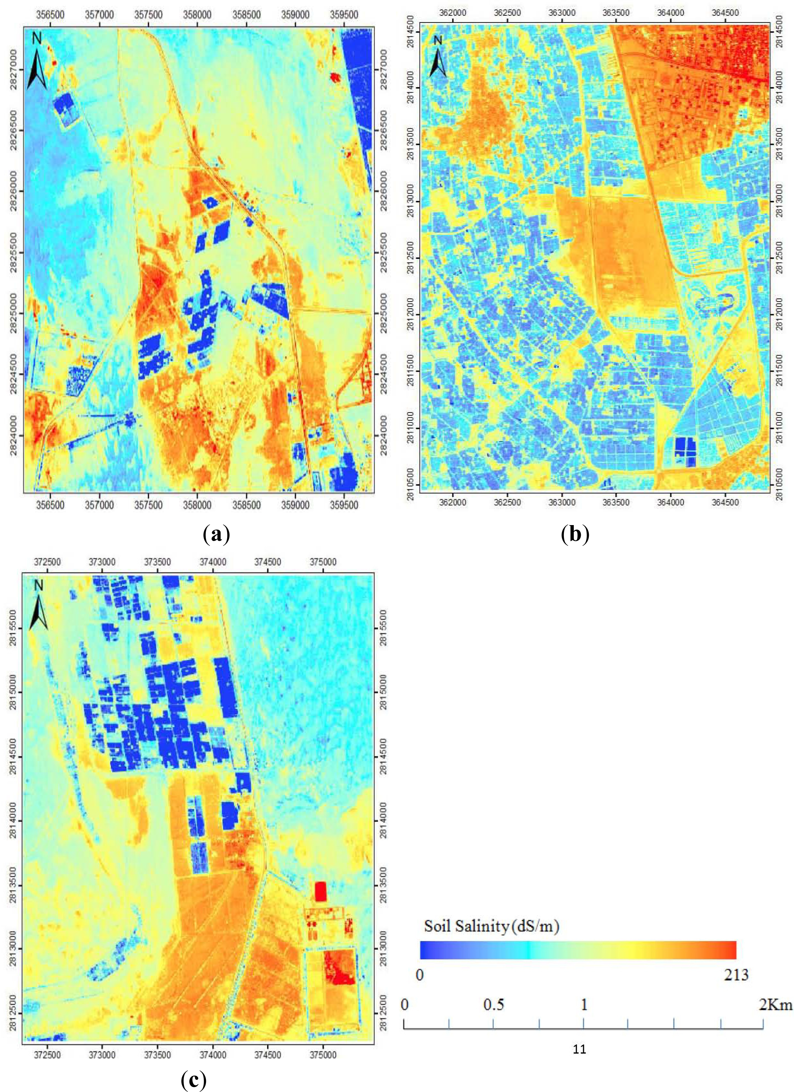
3.3. Spatial Variation in Soil Salinity Maps

Maps of the study areas generated using the selected model (model 4) are presented in Figure 4. In general, these maps show that most of the areas with very strongly saline soil (>16 dS/m) are non-vegetated, and areas with vegetation have soils with lower salinity levels, although still in the >16 dS/m class.

4. Discussion

4.1. The Developed Regressions Models

The efficiency of the selected regression model to predict and map the spatial variation in soil salinity is shown by the good relationship (R² = 0.65) at the 99% probability level, RMSE of 39 dS/m and the normality of the residuals. This is in part due to the high spatial resolution of the IKONOS images. The selected model in this study showed superiority in the prediction power (R² = 0.65) of soil salinity over those reported by Shrestha [27] (R² = 0.23) and recently by Shamsi et al. [35] (R² = 0.39), which have been developed using different moderate spatial resolution satellite images. Moderate spatial resolution images, such as the Advanced Spaceborne Thermal Emission and Reflection Radiometer (ASTER), Moderate Resolution Imaging Spectroradiometer (MODIS) and Landsat, are economically priced or free, more accessible and typically offer broader spatial coverage than more expensive high spatial resolution imagery. Nonetheless, differences in spatial resolution can have a high impact on predicting soil salinity. Our finding that the prediction of soil salinity based on IKONOS images yields better results than those based on moderate resolution images is in agreement with Eldeiry and Garcia [19]. Given this concern, it is important to take into account spatial resolution as one of the key factors to consider when using satellite imagery to infer soil salinity.

Moreover, the good performance of the selected model in this study is due to the enhanced images efficacy in highlighting information from soil salinity and suppressing the other details. Image enhancement is data processing that aims to increase the overall visual quality of an image or to enhance the visibility and interpretability of certain features of interest in it [53]. Several studies have shown that image enhancement techniques consisting of spectral indices (e.g., NDVI, SI, NDSI, TNDVI) have a great potential in enhancing and delineating soil salinity detail in an image [29,31,54–59]. For example, Tripathi et al. [49] found and emphasized that identifying salt-affected soils based on the image enhancement method, represented by the salinity index, yields better results than individual bands, due to its ability to enhance the saline patches by suppressing the vegetation. Recently, Shamsi et al. [35] conducted a study to characterise soil salinity in the south-east of Fars Province, Iran, using remote sensing and statistical analysis, and found that using an image enhancement method (Salinity Index (SI)) reduced estimation errors and increased the model’s efficiency.

Beside this, the superiority of the visible red band over the other bands in retrieving soil salinity has contributed to improving the regression model. This result is supported by those of Arasteh [60] and Mariappan [61] who found that the visible red band performs best among the Landsat ETM+ bands at characterizing the pattern and features of soil salinity due to its high correlation with EC ground measurements. Soil salinity spectral reflectance is affected by the physical-chemical properties of soil: quality and mineralogy of salt, together with soil moisture, colour and surface roughness [62]. Salts influenced surface features are crusts without or with only a little evidence of salt; thick salt crusts and puffy structures. Salt causes variations in the surface roughness which induces variation in the soil spectral reflectance [4,5,63]. Most salt-affected soils can be identified by a white salt crust that will form on the soil surface; thus, these soils tend to increase spectral reflectance [64–66]. Crusted soil, which affects soil structure and reduces the soil infiltration rate [67] is characterized with significant spectral changes due to the structural crust formation and colour [66]. Salt crust at its inception (high infiltration rate) presents low spectral reflectance, whereas in intense salt crust soil, the spectral reflectance will be significantly higher [66]. Besides, smooth crust surfaces have higher spectral reflectance than rougher crust surfaces [66,68–70].

According to the investigated samples in this study, saline soils with a smooth and light salty crust surface show high spectral reflectance in the red band, in contrast saline soils characterized by coarse dark puffy surface crust exhibit a decrease in spectral reflectance (Figure 5). These findings are in agreement with the those of Metternicht and Zinck [71], Schmid et al. [72] and Shamsi et al. [35], and confirm the fact that saline soil reflectance results from spectral properties such as the presence of salt crust, soil colour and moisture content, which have a combined effect on the amount of reflectance.

Thus, it is clear that a combination of spectral bands and image enhancement yield a better result than the actual band used for modelling and mapping soil salinity alone. This finding is consistent with those of Tajgardan et al. [36], Eldeiry and Garcia [19], Bouaziz et al. [37], Judkins and Myint [20] and Noroozi et al. [29], who found that this method of combining spectral bands with enhanced images in a single model is a promising tool for soil salinity detection and mapping. That is to say, the combination is the key, giving better results than either spectral band alone or image enhancement alone.

4.2. Mapping Spatial Variation in Soil Salinity

Factors causing soil salinity include inappropriate and excessive irrigation without an adequate drainage system, irrigation water quality, a rising water table, climate, rainfall history, local topography, soil composition and farming practices [73–77]. Therefore, increasing soil salinity at the surface is most likely to vary according to the distribution of these different factors across the landscape. For example, Bilgili [73] found that the spatial distribution of saline soils in the Harran Plain, southeast Turkey, is likely due to inappropriate irrigation coupled with high evaporation and topographical factors.

In this study, soil salinity maps that were generated using the selected model showed large surface areas with very strongly saline soil (>16 dS/m). The spatial distribution in this soil salinity class was variable over the investigated areas. Patches with strongly saline soil along the three sites were most pronounced in non-vegetated wet and dry areas. Wet areas, shown in red and orange colours in the maps (Figure 4), form due to a rising water table and are characterized by a moisture-filled soil [74]. The rising water table brings salt from deep in the soil up to the surface, causing salt accumulation [75]. On the other hand dry lands, which are shown in a colour graduation from yellow to light blue, occurs when a saline water table comes close to the ground level and a high evaporation rate leaves salts at the soil surface [76]. Thus, these findings suggested that a rising water table and salt accumulation at the surface combined with a high evaporation rate are one of the most likely factors that have resulted in the spatial variation in soil salinity over these lands. Similar results in an arid region, Sultanate Oman, were found by [77].

On the other hand, vegetated areas occupy strongly saline soil but within lower salinity levels compared to the non-vegetated areas. The lower observed salinity levels on the vegetated areas may occur because vegetated areas are subjected to a leaching process which reduces salinity levels. In spite of this, there were pronounced salinity differences between the three sites over the vegetated areas. These differences were potentially caused by variation in topography, soil type and structure, poor drainage and irrigation water quality. All of these parameters are known to affect soil salinity distribution across the landscape [77–81]. However, while irrigation water quality can be problematic, this can be overcome by proper irrigation management. Therefore, the observed salinity differences in the salinity levels on vegetated areas could be caused by different irrigation management practices, including irrigation scheduling. For example, instruments that measure and monitor soil moisture were not used for irrigation scheduling at any of the three study sites as farmers were not aware of them and/or lacked the required skills for use. In addition, many farmers cannot afford these instruments, and no extension services are available to encourage their use. Consequently, excessive water applications and poor timing result in various levels of salt build-up in these soils which adversely affect date palm. Several studies have found that soil salinity can cause significant effects on date palm growth and productivity, even though date palm is a high salt-tolerant crop [82–85]. Recently, Al-Abdoulhadi et al. [38] conducted a study to describe the effects of soil salinity on date palms. The results of their study revealed that salinity depressed plant growth and the biomass of date palms, and as the salinity increased the leaf length of the fronds was significantly reduced.

This study shows how regression analysis, coupled with high spatial resolution remote sensing images, could successfully predict and map spatial variation in soil salinity over an area vegetated mainly with date palms. Thus, the information presented here can help agricultural workers, scientists and engineers to manage soil salinity problems affecting the ecosystem. Additionally, the simplicity of this approach, with its satisfactory accuracy, can contribute greatly to soil salinity prediction and mapping, at lower costs than conventional approaches.

While, this study focuses on mapping and modelling soil salinity on a spatial variation basis at one point in time, further research requires investigating the temporal variation of soil salinity in this oasis in order to assess the pattern of soil salinity change over time as soil salinity is a space-time variation phenomena. This timely detection of soil salinity, prediction and mapping of its severity and extent will enable decision makers to decide what necessary actions should be taken, especially in areas of strongly saline soils, to protect the date palm outputs, sustain agricultural lands and natural ecosystems.

Besides, although this study contains promising results for modelling and mapping soil salinity based on regression analysis and IKONOS high spatial resolution images, the absence of the thermal band, which has been found a useful tool in several soil salinity studies [71,86,87], and the poor spectral resolution of the images, most likely limit the model capability. Thus, this study can be extended in the future by using hyperspectral images and investigating how this can increase the accuracy of spatial variation in similar modelling and mapping environments. Different studies have reported that hyperspectral images have a promising potential in the assessment and mapping of soil salinity [7,25,88–92]. For example, Weng et al. [88] found that soil salinity can be predicted and mapped successfully based on Partial Least Squares Regression (PLSR) techniques with Hyperion hypespectral data in a large area. More recently, in the Jezre’el Valley, northern Israel, Goldshleger et al. [5], based on PLSR techniques, assessed the relationships between salinity in tomato plants and soil spectral reflectance obtained using a hyperspectral radiometer and found that the results promising. They concluded that a hyperspectral radiometer is useful for characterizing salinity in growing vegetation and assessing its salt quality. To the best of our knowledge, hyperspectral remote sensing data have never been used to model and map soil salinity in communities vegetated mainly with date palms in the remote sensing domain. Therefore, further research is needed to investigate the capability of hyperspectral remote sensing data in mapping and modelling soil salinity under such conditions.

5. Conclusions

The present study demonstrates that combining the IKONOS red band and the salinity index into a regression model offers a potentially quick and inexpensive method to map and model the spatial variation in soil salinity of communities vegetated mostly with date palm. The combination of these remotely sensed variables into one model were able to explain 65% of the spatial variation in the soil salinity of the study area. The great capacity of this combined model over the other developed models is attributed to the enhanced images and the red band efficacy in highlighting information from soil salinity. The developed model’s simplicity and acceptable degree of accuracy makes it a promising tool for continued use in soil salinity prediction. Thus, this model can be used by the decision makers in Al Hassa oasis municipality and similar regions to implement or support effective soil reclamation programs that minimize or prevent future increases in soil salinity.

Although this study demonstrates that soil salinity mapping and modelling can be undertaken with good accuracy based on high spatial resolution multispectral images, further research is needed to focus on investigating the possibility of hyperspectral data in mapping and modelling soil salinity over areas dominated by date palm and investigating whether it can increase the accuracy of modelling and the mapping process.

References

1. Tanji, K. Salinity in the Soil Environment. In Salinity: Environment-Plants-Molecules; Lauchli, A., Luttge, U., Eds.; Kluwer Academic Publisher: Dordrecht, The Netherlands, 2004; pp. 21–51. [Google Scholar]
2. Jordán, M.; Navarro-Pedreño, J.; García-Sánchez, E.; Mateu, J.; Juan, P. Spatial dynamics of soil salinity under arid and semi-arid conditions: Geological and environmental implications. Environ. Geol 2004, 45, 448–456. [Google Scholar]
3. Douaik, A.; Meirvenne, M.; Toth, T. Stochastic Approaches for Space–Time Modeling and Interpolation of Soil Salinity. In Remote Sensing of Soil Salinization: Impact on Land Management; Metternicht, G., Zinck, J.A., Eds.; CRC Press: Boca Raton, FL, USA, 2008; pp. 273–289. [Google Scholar]
4. Ben-Dor, E.; Goldshleger, N.; Eshel Mor, V. Combined Active and Passive Remote Sensing Methods for Assessing Soil Salinity: A Case Study from Jezre’el Valley, Northern Israel. In Remote Sensing of Soil Salinization: Impact on Land Management; Metternicht, G., Zinck, J.A., Eds.; CRC Press: Boca Raton, FL, USA, 2008; pp. 236–253. [Google Scholar]
5. Goldshleger, N.; Chudnovsky, A.; Ben-Binyamin, R. Predicting salinity in tomato using soil reflectance spectra. Int. J. Remote Sens 2013, 34, 6079–6093. [Google Scholar]
6. Metternicht, G.; Zinck, A. Remote Sensing of Soil Salinization: Impact on Land Management; CRC Press: Boca Raton, FL, USA, 2008; p. 377. [Google Scholar]
7. Farifteh, J.; van der Meer, F.; Atzberger, C.; Carranza, E. Quantitative analysis of salt-affected soil reflectance spectra: A comparison of two adaptive methods (PLSR and ANN). Remote Sens. Environ 2007, 110, 59–78. [Google Scholar]
8. Akramkhanov, A.; Vlek, P. The assessment of spatial distribution of soil salinity risk using neural network. Environ. Monit. Assess 2012, 184, 2475–2485. [Google Scholar]
9. Patel, R.; Prasher, S.; God, P.; Bassi, R. Soil salinity prediction using artificial neural networks. J. Am. Water Resour. Assoc 2002, 38, 91–100. [Google Scholar]
10. Fethi, B.; Magnus, P.; Ronny, B.; Akissa, B. Estimating soil salinity over a shallow saline water table in semiarid Tunisia. Open Hydrol. J 2010, 4, 91–101. [Google Scholar]
11. Taghizadeh-Mehrjardi, R.; Minasny, B.; Sarmadian, F.; Malone, B. Digital mapping of soil salinity in Ardakan region, central Iran. Geoderma 2014, 213, 15–28. [Google Scholar]
12. Tóth, T.; Pasztor, L.; Kabos, S.; Kuti, L. Statistical prediction of the presence of salt-affected soils by using digitalized hydrogeological maps. Arid Land Res. Manag 2002, 16, 55–68. [Google Scholar]
13. Malins, D.; Metternicht, G. Assessing the spatial extent of dryland salinity through fuzzy modeling. Ecol. Model 2006, 193, 387–411. [Google Scholar]
14. Douaik, A.; van Meirvenne, M.; Toth, T.; Serre, M. Space-time mapping of soil salinity using probabilistic bayesian maximum entropy. Stoch. Environ. Res. Risk Assess 2004, 18, 219–227. [Google Scholar]
15. Triantafilis, J.; Odeh, I.; McBratney, A. Five geostatistical models to predict soil salinity from electromagnetic induction data across irrigated cotton. Soil Sci. Soc. Am. J 2001, 65, 869–878. [Google Scholar]
16. Tajgardan, T.; Ayoubi, S.; Shataee, S.; Sahrawat, K.L.; Gorgan, I. Soil surface salinity prediction using ASTER data: Comparing statistical and geostatistical models. Aust. J. Basic Appl. Sci 2010, 4, 457–467. [Google Scholar]
17. Eldeiry, A.A.; García, L.A. Using Deterministic and Geostatistical Techniques to Estimate Soil Salinity at the Sub-Basin Scale and the Field Scale. Proceedings of the 31th Annual Hydrology Days, Fort Collins, CO, USA, 21–23 March 2011.
18. Douaoui, A.E.K.; Nicolas, H.; Walter, C. Detecting salinity hazards within a semiarid context by means of combining soil and remote-sensing data. Geoderma 2006, 134, 217–230. [Google Scholar]
19. Eldeiry, A.A.; Garcia, L.A. Detecting soil salinity in alfalfa fields using spatial modeling and remote sensing. Soil Sci. Soc. Am. J 2008, 72, 201–211. [Google Scholar]
20. Judkins, G.; Myint, S. Spatial variation of soil salinity in the Mexicali valley, Mexico: Application of a practical method for agricultural monitoring. Environ. Manag 2012, 50, 478–489. [Google Scholar]
21. Fan, X.; Pedroli, B.; Liu, G.; Liu, Q.; Liu, H.; Shu, L. Soil salinity development in the yellow river delta in relation to groundwater dynamics. Land Degrad. Dev 2012, 23, 175–189. [Google Scholar]
22. McBratney, A.; Santos, M.d.L.M.; Minasny, B. On digital soil mapping. Geoderma 2003, 117, 3–52. [Google Scholar]
23. Scull, P.; Franklin, J.; Chadwick, O.; McArthur, D. Predictive soil mapping: A review. Progr. Phys. Geogr 2003, 27, 171–197. [Google Scholar]
24. Lesch, S.M.; Strauss, D.J.; Rhoades, J.D. Spatial prediction of soil salinity using electromagnetic induction techniques: 1. Statistical prediction models: A comparison of multiple linear regression and cokriging. Water Resour. Res 1995, 31, 373–386. [Google Scholar]
25. Yonghua, Q.; Siongb, J.; Xudonga, L. A Partial Least Square Regression Method to Quantitatively Retrieve Soil Salinity using Hyper-Spectral Reflectance Data. Proceedings of the SPIE 7147, Geoinformatics 2008 and Joint Conference on GIS and Built Environment: Classification of Remote Sensing Images, Guangzhou, China, 31 October 2008.
26. Wang, H.; Wang, J.; Liu, G. Spatial Regression Analysis on the Variation of Soil Salinity in the Yellow River Delta. Proceedings of the SPIE 6753, Geoinformatics 2007: Geospatial Information Science, Nanjing, China, 10 June 2007.
27. Shrestha, R. Relating soil electrical conductivity to remote sensing and other soil properties for assessing soil salinity in northeast Thailand. Land Degrad. Dev 2006, 17, 677–689. [Google Scholar]
28. Pakparvar, M.; Gabriels, D.; Aarabi, K.; Edraki, M.; Raes, D.; Cornelis, W. Incorporating legacy soil data to minimize errors in salinity change detection: A case study of Darab Plain, Iran. Int. J. Remote Sens 2012, 33, 6215–6238. [Google Scholar]
29. Noroozi, A.A.; Homaee, M.; Farshad, A. Integrated application of remote sensing and spatial statistical models to the identification of soil salinity: A case study from Garmsar Plain, Iran. Environ. Sci 2012, 9, 59–74. [Google Scholar]
30. Mehrjardi, R.T.; Mahmoodi, S.H.; Taze, M.; Sahebjalal, E. Accuracy assessment of soil salinity map in Yazd-Ardakan Plain, Central Iran, based on Landsat ETM+ imagery. Am.-Eurasian J. Agric. Environ. Sci 2008, 3, 708–712. [Google Scholar]
31. Fernandez-Buces, N.; Siebe, C.; Cram, S.; Palacio, J. Mapping soil salinity using a combined spectral response index for bare soil and vegetation: A case study in the former lake Texcoco, Mexico. J. Arid Environ 2006, 65, 644–667. [Google Scholar]
32. Eldeiry, A.A.; Garcia, L.A. Spatial modeling using remote sensing, GIS, and field data to assess crop yield and soil salinity. Hydrol. Days 2004, 7, 55–66. [Google Scholar]
33. Afework, M. Analysis and Mapping of Soil Salinity Levels in Metehara Sugarcane Estate Irrigation Farm Using Different Models. Addis Ababa University, Ethiopia, Addis Ababa, 2009. [Google Scholar]
34. Weng, Y.; Gong, P.; Zhu, Z. Reflectance spectroscopy for the assessment of soil salt content in soils of the Yellow River Delta of China. Int. J. Remote Sens 2008, 29, 5511–5531. [Google Scholar]
35. Shamsi, F.R.S.; Sanaz, Z.; Abtahi, A.S. Soil salinity characteristics using moderate resolution imaging spectroradiometer (MODIS) images and statistical analysis. Arch. Agron. Soil Sci 2013, 59, 471–489. [Google Scholar]
36. Tajgardan, T.; Shataee, S.; Ayoubi, S. In Spatial Prediction of Soil Salinity in the Arid Zones Using ASTER Data, Case study: North of Ag Ghala, Golestan Province, Iran. Proceedings of Asian Conference on Remote Sensing (ACRS), Kuala Lumpur, Malaysia, 12–16 November 2007.
37. Bouaziz, M.; Matschullat, J.; Gloaguen, R. Improved remote sensing detection of soil salinity from a semi-arid climate in Northeast Brazil. Comptes Rendus Geosci 2011, 343, 795–803. [Google Scholar]
38. Al-Abdoulhadi, I.A.; Dinar, H.A.; Ebert, G.; Bttner, C. Effect of salinity on leaf growth, leaf injury and biomass production in date palm (Phoenix dactylifera L.) cultivars. Indian J. Sci. Technol 2011, 4, 1542–1546. [Google Scholar]
39. Al-Dakheel, Y.; Massoud, M. Towards Sustainable Development for Groundwater in Al-Hassa and the Role of Geographic Information Systems. Proceeidngs of the The 2nd International Conference on Water Resources & Arid Environment, Riyadh, Saudi Arabia, 26–29 November 2006.
40. Hussain, G.; Al-Zarah, A.I.; Latif, M.S. Influence of groundwater irrigation on chemical properties of soils in the vicinity of wastewater drainage canals in Al-Alisa Oasis. Res. J. Environ. Toxicol. (RJET) 2012, 7, 1–17. [Google Scholar]
41. Al-Naeem, A.A. Evaluation of groundwater of al-hassa oasis, eastern region Saudi Arabia. Res. J. Environ. Sci 2011, 5, 624–642. [Google Scholar]
42. Al Tokhais, A.S.; Rausch, R. In The Hydrogeology of Al Hassa Springs. Proceedings the 3rd International Conference on Water Resources and Arid Environments and the 1 Arab Water Forum, st Riyadh, Saudi Arabia, 16–19 November 2008; pp. 16–19.
43. AI-Barrak, S.A. Characteristics of some soils under date palm in AI-Hassa eastern oasis, Saudi Arabia. J. King Saud Univ. Agric. Sci 1990, 2, 115–130. [Google Scholar]
44. Elprince, A.M. Model for the soil solution composition of an oasis. Soil Sci. Soc. Am. J 1985, 49, 1121–1128. [Google Scholar]
45. Bouaziz, M.; Gloaguena, R.; Samirb, B. Remote mapping of susceptible areas to soil salinity, based on hyperspectral data and geochemical, in the Southern Part of Tunisia. Proc. SPIE 2011, 8174. [Google Scholar] [CrossRef]
46. Richards, L. Determination of the Properties of Saline and Alkali Soils. In Diagnosis and Improvement of Saline and Alkali Soils, Agriculture Handbook No. 60; US Regional Salinity Laboratory: Riverside, CA, USA, 1954; pp. 7–33. [Google Scholar]
47. Dial, G.; Bowen, H.; Gerlach, F.; Grodecki, J.; Oleszczuk, R. IKONOS satellite, imagery, and products. Remote Sens. Environ 2003, 88, 23–36. [Google Scholar]
48. Chavez, P.S., Jr. Image-based atmospheric corrections-revisited and improved. Photogramm. Eng. Remote Sens 1996, 62, 1025–1035. [Google Scholar]
49. Tripathi, N.K.; Rai, B.K.; Dwivedi, P. Spatial modelling of soil alkalinity in GIS environment using IRS data. Proceedings of the 18th Asian Conference in Remote Sensing, ACRS Kuala Lumpur, Malaysia, 20–25 October 1997; pp. 81–86.
50. Royston, P.; Sauerbrei, W. Multivariable Model-Building: A Pragmatic Approach to Regression Anaylsis Based on Fractional Polynomials for Modelling Continuous Variables; John Wiley & Sons: Chichester, UK, 2008; p. 322. [Google Scholar]
51. Moriasi, D.; Arnold, J.; van Liew, M.; Bingner, R.; Harmel, R.; Veith, T. Model evaluation guidelines for systematic quantification of accuracy in watershed simulations. Trans. ASABE 2007, 50, 885–900. [Google Scholar]
52. Field, A.; Miles, J.; Field, Z. Discovering Statistics Using R; SAGE Publications: London, UK, 2012; p. 992. [Google Scholar]
53. Gao, J. Digital Analysis of Remotely Sensed Imagery, 1st ed; McGraw Hill Professional: New York, NY, USA, 2008; p. 674. [Google Scholar]
54. Odeh, I.O.; Onus, A. Spatial analysis of soil salinity and soil structural stability in a semiarid region of New South Wales, Australia. Environ. Manag 2008, 42, 265–278. [Google Scholar]
55. Iqbal, F. Detection of salt affected soil in rice-wheat area using satellite image. Afr. J. Agric. Res 2011, 6, 4973–4982. [Google Scholar]
56. Khan, N.M.; Rastoskuev, V.V.; Sato, Y.; Shiozawa, S. Assessment of hydrosaline land degradation by using a simple approach of remote sensing indicators. Agric. Water Manag 2005, 77, 96–109. [Google Scholar]
57. Lobell, D.; Lesch, S.; Corwin, D.; Ulmer, M.; Anderson, K.; Potts, D.; Doolittle, J.; Matos, M.; Baltes, M. Regional-scale assessment of soil salinity in the Red River Valley using multi-year MODIS EVI and NDVI. J. Environ. Qual 2010, 39, 35–41. [Google Scholar]
58. Hamzeh, S.; Naseri, A.A.; AlaviPanah, S.K.; Mojaradi, B.; Bartholomeus, H.M.; Clevers, J.; Behzad, M. Estimating salinity stress in sugarcane fields with spaceborne hyperspectral vegetation indices. Int. J. Appl. Earth Obs. Geoinformation 2012, 21, 282–290. [Google Scholar]
59. Naumann, J.C.; Young, D.R.; Anderson, J.E. Spatial variations in salinity stress across a coastal landscape using vegetation indices derived from hyperspectral imagery. Plant Ecol 2009, 202, 285–297. [Google Scholar]
60. Arasteh, P.D. Soil Salinity Change Detection in Irrigated Area Under Gazvin Plain Irrigation Network Using Satellite Imagery. Proceedings of the 9th International Drainage Symposium, Québec City, QC, Canada, 13–16 June 2010; pp. 1–9.
61. Mariappan, V.E.N. Soil salinity assessment using geospatial technology, perspectives, approaches and sctrategies. Indian Cartogr 2010, 30, 25–30. [Google Scholar]
62. Metternicht, G.; Zinck, J.A. Spectral Behavior of Salt Types. In Remote Sensing of Soil Salinization: Impact on Land Management; Metternicht, G., Zinck, J.A., Eds.; CRC Press: Boca Raton, FL, USA, 2008; pp. 21–36. [Google Scholar]
63. Goldshleger, N.; Livne, I.; Chudnovsky, A.; Ben-Dor, E. New results in integrating passive and active remote sensing methods to assess soil salinity: A case study from Jezre’el Valley, Israel. Soil Sci 2012, 177, 392–401. [Google Scholar]
64. Panah, S.K.A.; Goossens, R.; Matinfar, H.R.; Mohamadi, H.; Ghadiri, M.; Irannegad, H.; Asl, M.A. The efficiency of Landsat TM and ETM+ thermal data for extracting soil information in arid regions. J. Agric. Sci. Technol 2008, 10, 439–460. [Google Scholar]
65. De Jong, S.M.; Addink, E.A.; van Beek, L.P.H.; Duijsings, D. Physical characterization, spectral response and remotely sensed mapping of Mediterranean soil surface crusts. Catena 2011, 86, 24–35. [Google Scholar]
66. Ben-Dor, E.; Goldlshleger, N.; Benyamini, Y.; Agassi, M.R.; Blumberg, D.G. The spectral reflectance properties of soil structural crusts in the 1.2-to 2.5-μm spectral region. Soil Sci. Soc. Am. J 2003, 67, 289–299. [Google Scholar]
67. Agassi, M.; Morin, J.; Shainberg, I. Effect of raindrop impact energy and water salinity on infiltration rates of sodic soils. Soil Sci. Soc. Am. J 1985, 49, 186–190. [Google Scholar]
68. Metternicht, G.I.; Zinck, J.A. Remote sensing of soil salinity: Potentials and constraints. Remote Sens. Environ 2003, 85, 1–20. [Google Scholar]
69. Elnaggar, A.A.; Noller, J.S. Application of remote-sensing data and decision-tree analysis to mapping salt-affected soils over large areas. Remote Sens 2010, 2, 151–165. [Google Scholar]
70. Goldshleger, N.; Ben-Dor, E.; Benyamini, Y.; Agassi, M. Soil reflectance as a tool for assessing physical crust arrangement of four typical soils in Israel. Soil Sci 2004, 169, 677–687. [Google Scholar]
71. Metternicht, G.; Zinck, J. Spatial discrimination of salt-and sodium-affected soil surfaces. Int. J. Remote Sens 1997, 18, 2571–2586. [Google Scholar]
72. Schmid, T.; Koch, M.; Gumuzzio, J. Applications of Hyper-Spectral Imagery to Soil Salinity Mapping. In Remote Sensing of Soil Salinization: Impact on Land Management; Metternicht, G., Zinck, J., Eds.; CRC Press: Boca Raton, FL, USA, 2009; pp. 113–140. [Google Scholar]
73. Bilgili, A.V. Spatial assessment of soil salinity in the Harran Plain using multiple kriging techniques. Environ. Monit. Assess 2013, 185, 777–795. [Google Scholar]
74. Keddy, P.A. Wetland Ecology: Principles and Conservation; Cambridge University Press: Cambridge, UK, 2010; p. 497. [Google Scholar]
75. Ashraf, M.; Öztürk, M.A.; Athar, H.R. Salinity and Water Stress: Improving Crop Efficiency; Springer: Dordrecht, The Netherlands, 2009; p. 260. [Google Scholar]
76. Jardine, A.; Speldewinde, P.; Carver, S.; Weinstein, P. Dryland salinity and ecosystem distress syndrome: Human health implications. EcoHealth 2007, 4, 10–17. [Google Scholar]
77. Hussain, N.; Al-Rawahy, A.S.; Rabee, J.; Al-Amri, M. Causes, origin, genesis and extent of soil salinity in the Sultanate of Oman. Pak. J. Agric. Sci 2006, 43, 1–2. [Google Scholar]
78. Thiruchelvam, S.; Pathmarajah, S. An Economic Analysis of Salinity Problems in the Mahaweli River System H Irrigation Scheme in Sri Lanka; Economy and Environment Program for Southeast Asia (EEPSEA): Ottawa, Canada, 1999; p. 39. [Google Scholar]
79. Cetin, M.; Kirda, C. Spatial and temporal changes of soil salinity in a cotton field irrigated with low-quality water. J. Hydrol 2003, 272, 238–249. [Google Scholar]
80. Zheng, Z.; Zhang, F.; Ma, F.; Chai, X.; Zhu, Z.; Shi, J.; Zhang, S. Spatiotemporal changes in soil salinity in a drip-irrigated field. Geoderma 2009, 149, 243–248. [Google Scholar]
81. Sakadevan, K.; Nguyen, M.-L. Extent, impact, and response to soil and water salinity in arid and semiarid regions. Adv. Agron 2010, 109, 55–74. [Google Scholar]
82. Alhammadi, M.; Glenn, E. Detecting date palm trees health and vegetation greenness change on the eastern coast of the United Arab Emirates using SAVI. Int. J. Remote Sens 2008, 29, 1745–1765. [Google Scholar]
83. Ramoliya, P.; Pandey, A. Soil salinity and water status affect growth of Phoenix dactylifera seedlings. N. Z. J. Crop Hortic. Sci 2003, 31, 345–353. [Google Scholar]
84. Alhammadi, M.S.; Edward, G.P. Effect of salinity on growth of twelve cultivars of the United Arab Emirates date palm. Commun. Soil Sci. Plant Anal 2009, 40, 2372–2388. [Google Scholar]
85. Hussein, A.; El-Desouki, M.; El-Kased, F.; Nour, G.; Abd-El-Hamid, N. Effect of salinity on date palm seeds germination and early seedling growth. J. Agric. Sci. Mansoura Univ 1993, 18, 1306–1314. [Google Scholar]
86. Verma, K.; Saxena, R.; Barthwal, A.; Deshmukh, S. Remote sensing technique for mapping salt affected soils. Int. J. Remote Sens 1994, 15, 1901–1914. [Google Scholar]
87. Alavipanah, S.K.; Goossens, R. Relationship between the Landsat TM, MSS data and soil salinity. J. Agric. Sci. Technol 2001, 3, 101–111. [Google Scholar]
88. Weng, Y.; Gong, P.; Zhu, Z. Soil salt content estimation in the Yellow River delta with satellite hyperspectral data. Can. J. Remote Sens 2008, 34, 259–270. [Google Scholar]
89. Lu, N.; Zhang, Z.; Gao, Y. Recognition and Mapping of Soil Salinization in Arid Environment with Hyperspectral Data. Proceedings of the IGARSS’05. IEEE International Geoscience and Remote Sensing Symposium, Seoul, Korea, 25–29 July 2005; pp. 4520–4523.
90. Ben-Dor, E.; Patkin, K.; Banin, A.; Karnieli, A. Mapping of several soil properties using DAIS-7915 hyperspectral scanner data-a case study over clayey soils in Israel. Int. J. Remote Sens 2002, 23, 1043–1062. [Google Scholar]
91. Zhang, T.T.; Zeng, S.L.; Gao, Y.; Ouyang, Z.T.; Li, B.; Fang, C.M.; Zhao, B. Using hyperspectral vegetation indices as a proxy to monitor soil salinity. Ecol. Indic 2011, 11, 1552–1562. [Google Scholar]
92. Hamzeh, S.; Naseria, A.A.; Panah, S.K.A.; Mojaradic, B.; Bartholomeus, H.M.; Herold, M. Mapping salinity stress in sugarcane fields with hyperspecteral satellite imagery. Proc. SPIE 2012. [Google Scholar] [CrossRef]
Figure 1. Study area with the location of the study sites.
Remotesensing 06 01137f1
Figure 2. Scatter plots of predicted vs. measured EC using the developed regression models.
Remotesensing 06 01137f2aRemotesensing 06 01137f2b
Figure 3. Validation of the developed regression models: (a) scatterplots of the predicted vs. measured EC; (b) the histogram of the residuals; (c) the normal plot of the residuals.
Remotesensing 06 01137f3
Figure 4. Soil salinity maps for different sites in the study region: (a) site one; (b) site two; and (c) site three.
Remotesensing 06 01137f4
Figure 5. Spectral reflectance of saline soils differs due to surface roughness, crusting and colour.
Remotesensing 06 01137f5