The Generalized Difference Vegetation Index (GDVI) for Dryland Characterization †

Abstract
:1. Introduction
2. Materials and Methods
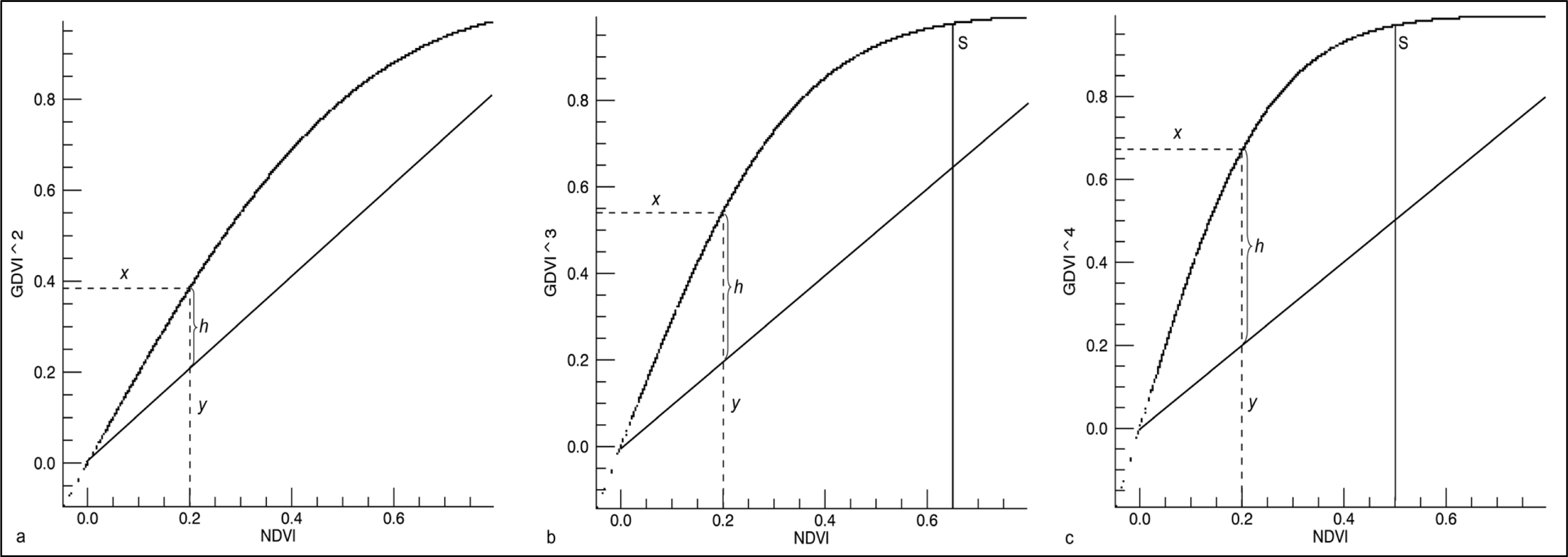
2.1. Rationale
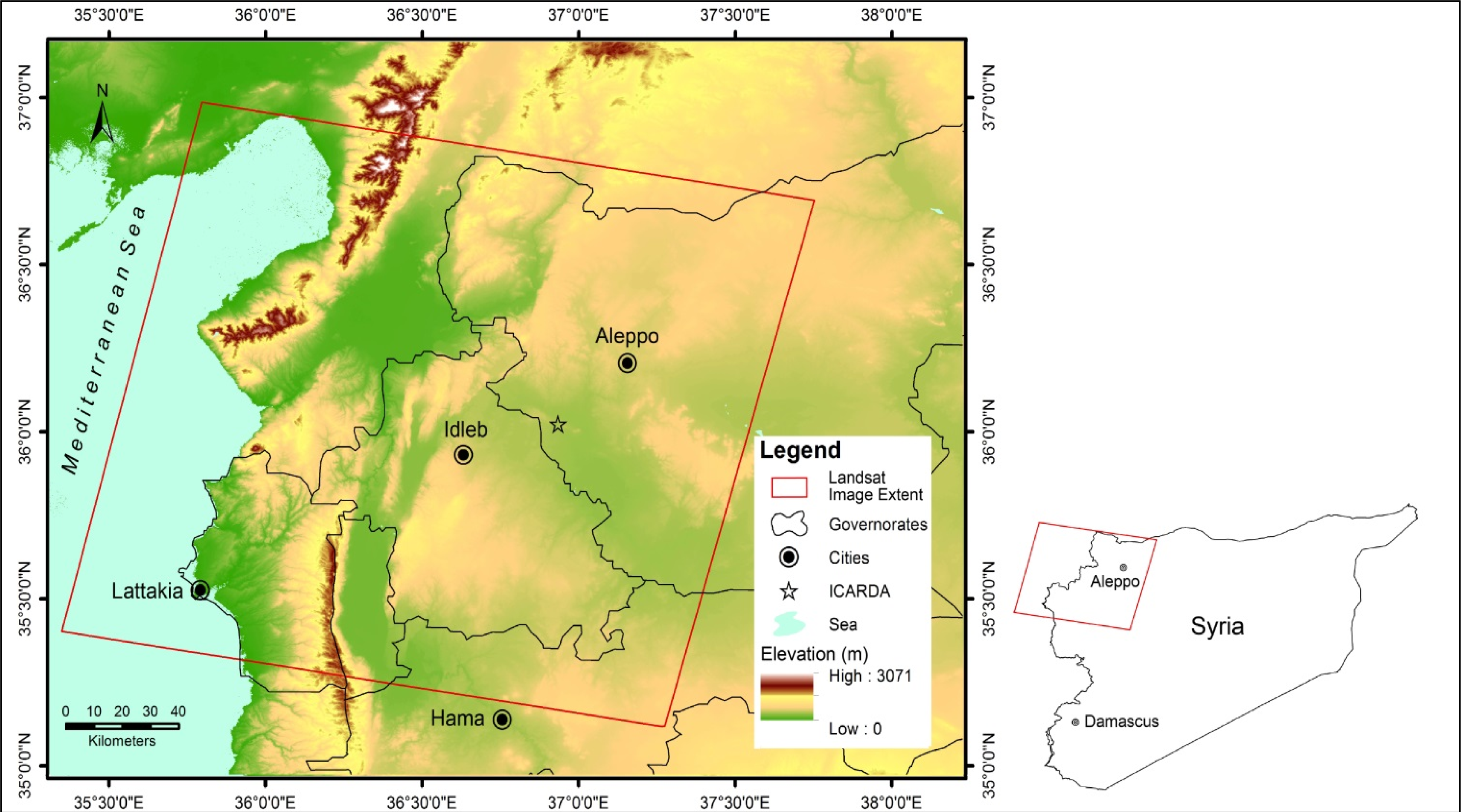
2.2. Test Site
2.3. Data
2.4. Evaluation Procedure
2.4.1. Atmospheric Correction
2.4.2. Calculation of Different Vegetation Indices and FVC
2.4.3. Selection of Sampling Areas
2.4.4. Calculation of the Mean Values and the Random Point Values of Different VIs in the Sampling Areas
2.4.5. Calibration
2.4.6. Sensitivity Analysis
3. Results and Discussions
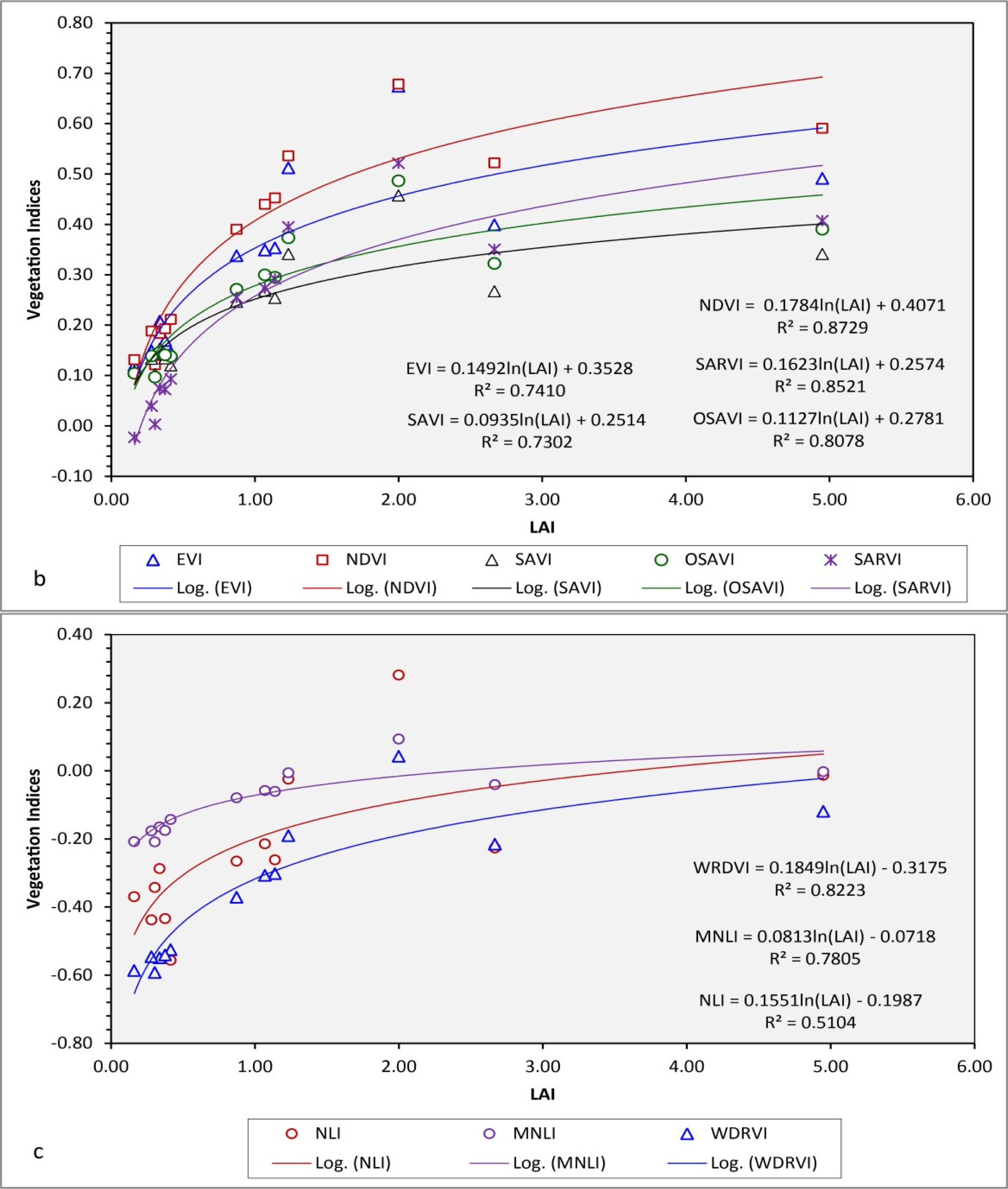
3.1. GDVI vs. LAI
3.1.1. Advantages
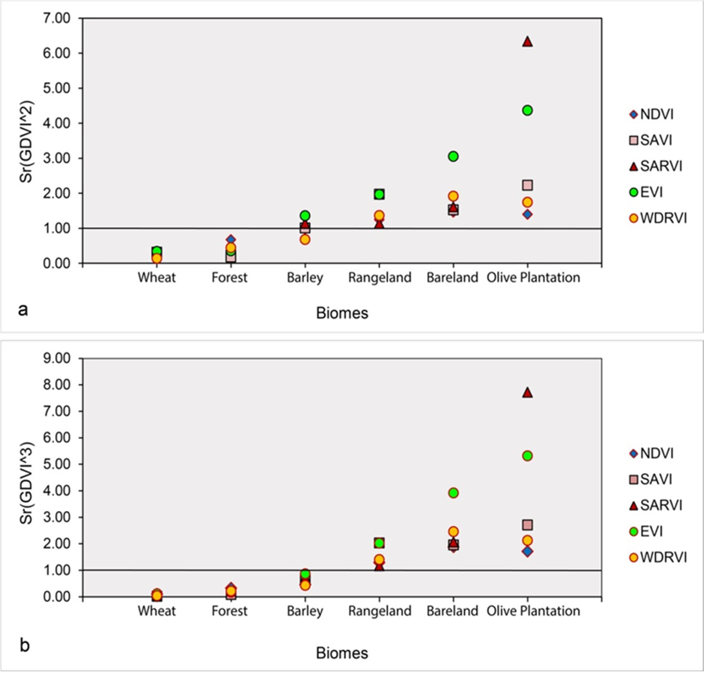
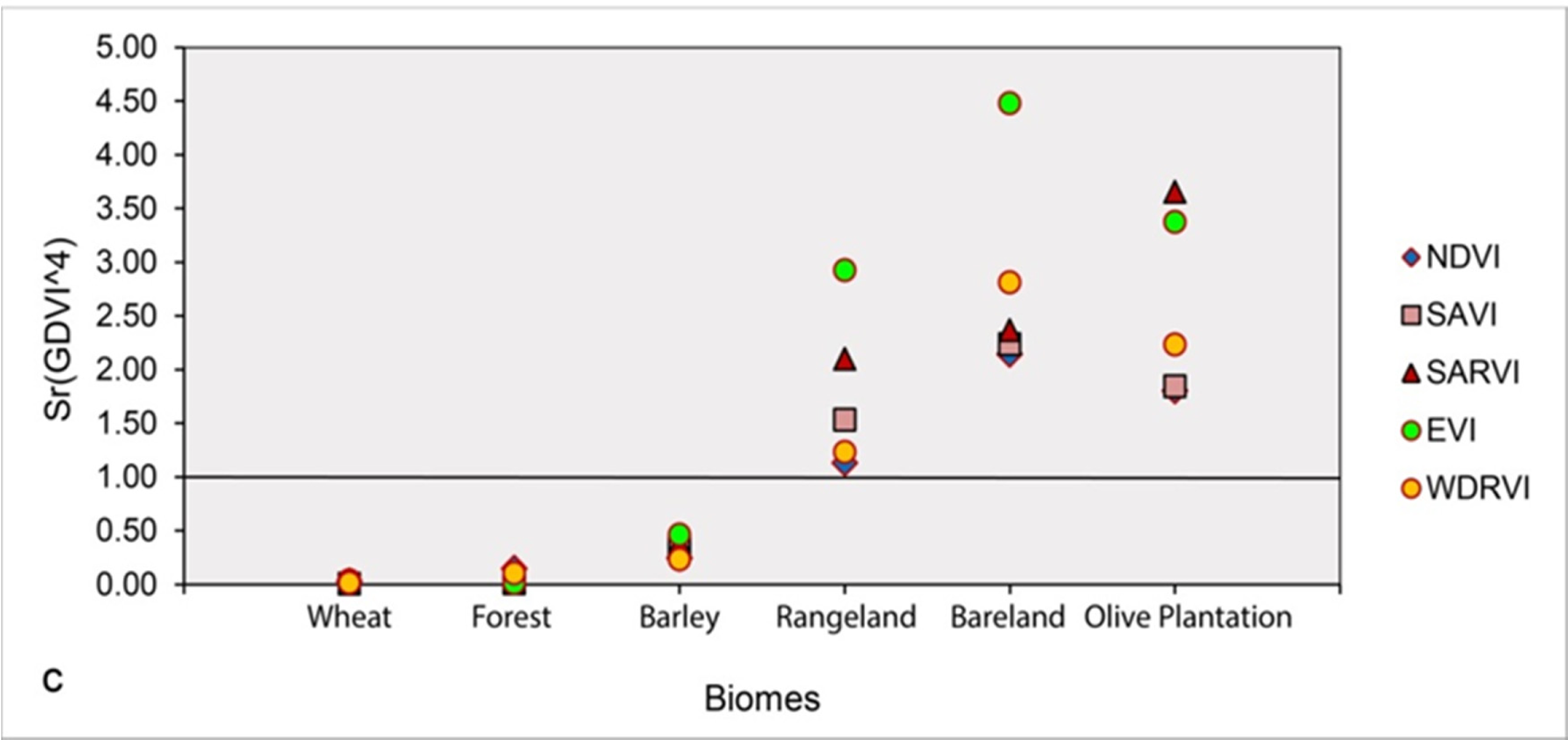
3.1.2. Sensitivity
3.2. GDVI vs. FVC
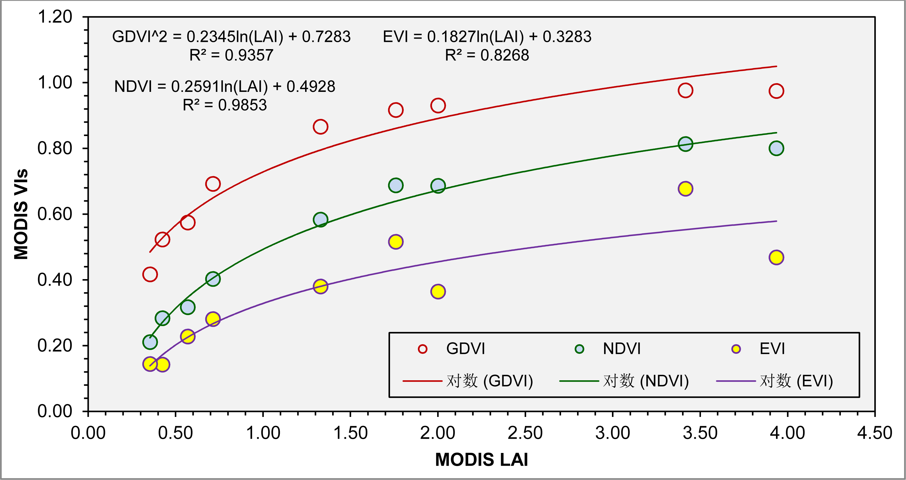
3.3. MODIS GDVI vs. MODIS LAI
3.4. Discussion on Limitation and Problems Encountered
4. Conclusions
Acknowledgments
Conflicts of Interest
References
- Tucker, C.J. Red and photographic infrared linear combinations for monitoring vegetation. Remote Sens. Environ. 1979, 8, 127–150. [Google Scholar]
- Vina, A.; Gitelson, A.A.; Nguy-Robertson, A.L.; Peng, Y. Comparison of different vegetation indices for the remote assessment of green leaf area index of crops. Remote Sens. Environ. 2011, 115, 3468–3478. [Google Scholar]
- Jiang, Z.; Huete, A.R.; Didan, K.; Miura, T. Development of a two-band enhanced vegetation index without a blue band. Remote Sens. Environ. 2008, 112, 3833–3845. [Google Scholar]
- Birth, G.S.; McVey, G.R. Measuring the color of growing turf with a reflectance spectrophotometer. Agron. J. 1968, 60, 640–643. [Google Scholar]
- Jordan, C.F. Derivation of leaf-area index from quality of light on the forest floor. Ecology 1969, 50, 663–666. [Google Scholar]
- Knipling, E.B. Physical and physiological bases for the reference of visible and near infrared radiation from vegetation. Remote Sens. Environ. 1970, 1, 155–159. [Google Scholar]
- Rouse, J.W.; Haas, R.H.; Schell, J.A.; Deering, D.W. Monitoring Vegetation Systems in the Great plains with ERTS. Proceedings of the 3rd ERTS-1 Symposium NASA SP-351, Washington, DC, USA, 10–14 December 1973; 1, pp. 309–317.
- Deering, D.W.; Rouse, J.W.; Haas, R.H.; Schel, J.A. Measuring Forage Production of Grazing Units from Landsat MSS Data. Proceedings of the 10th International Symposium of Remote Sensing of Environment, Ann Arbor, MI, USA, 6–10 October 1975; II, pp. 1169–1178.
- Richardson, A.J.; Wiegand, C.L. Distinguishing vegetation from soil background information. Photogramm. Eng. Remote Sens. 1977, 43, 1541–1552. [Google Scholar]
- Clevers, J.G.P.W. The derivation of a simplified reflectance model for the estimation of leaf area index. Remote Sens. Environ. 1988, 35, 53–70. [Google Scholar]
- Clevers, J.G.P.W. Application of the WDVI in estimating LAI at the generative stage of barley. ISPRS J. Photogramm. Remote Sens. 1991, 46, 37–47. [Google Scholar]
- Goel, N.S.; Qin, W. Influences of canopy architecture on relationships between various vegetation indices and LAI and FPAR: A computer simulation. Remote Sens. Rev. 1994, 10, 309–347. [Google Scholar]
- Gitelson, A.A.; Kaufman, Y.J.; Stark, R.; Rundquist, D. Novel algorithms for remote estimation of vegetation fraction. Remote Sens. Environ. 2002, 80, 76–87. [Google Scholar]
- Motohka, T.; Nasahara, K.N.; Oguma, H.; Tsuchida, S. Applicability of green-red vegetation index for remote sensing of vegetation phenology. Remote Sens. 2010, 2, 2369–2387. [Google Scholar]
- Gitelson, A.A. Wide dynamic range vegetation index for remote quantification of crop biophysical characteristics. J. Plant Physiol. 2004, 161, 165–173. [Google Scholar]
- Pinty, B.; Verstraete, M.M. GEMI: A non-linear index to monitor global vegetation from satellites. Plant Ecol. 1992, 101, 15–20. [Google Scholar]
- Huete, A.R. A soil adjusted vegetation index (SAVI). Remote Sens. Environ. 1988, 25, 295–309. [Google Scholar]
- Baret, F.; Guyot, G.; Major, D. TSAVI: A Vegetation Index which Minimizes Soil Brightness Effects on LAI and APAR Estimation. Proceedings of the 12th International Canadian Symposium Geoscience and Remote Sensing (IGARSS’89), Vancouver, BC, Canada, 10–14 July 1989; pp. 1355–1358.
- Qi, J.; Chehbouni, A.; Huete, A.R.; Kerr, Y.H.; Sorooshian, S. A modified soil adjusted vegetation index. Remote Sens. Environ. 1994, 48, 119–126. [Google Scholar]
- Rondeaux, G.; Steven, M.; Baret, F. Optimization of soil-adjusted vegetation index. Remote Sens. Environ. 1996, 55, 95–107. [Google Scholar]
- Gilabert, M.A.; Gonzalez-Piqueras, J.; Garcia-Haro, F.J.; Melia, J. A generalized soil-adjusted vegetation index. Remote Sens. Environ. 2002, 82, 303–310. [Google Scholar]
- Sripada, R.P.; Heiniger, R.W.; White, J.G.; Meijer, A.D. Aerial color infrared photography for determining early in-season nitrogen requirements in corn. Agron. J. 2006, 98, 968–977. [Google Scholar]
- Gong, P.; Pu, R.; Biging, G.S.; Larrieu, M.R. Estimation of forest leaf area index using vegetation indices derived from Hyperion hyperspectral data. IEEE Trans. Geosci. Remote Sens. 2003, 41, 1355–1362. [Google Scholar]
- Kaufman, Y.J.; Tanré, D. Atmospherically resistant vegetation index (ARVI) for EOS-MODIS. IEEE Trans. Geosci. Remote Sens. 1992, 30, 261–270. [Google Scholar]
- Huete, A.R.; Liu, H.Q.; Batchily, K.; van Leeuwen, W. A comparison of vegetation indices global set of TM images for EOS-MODIS. Remote Sens. Environ. 1997, 59, 440–451. [Google Scholar]
- Huete, A.; Didan, K.; Miura, T.; Rodriguez, E.P.; Gao, X.; Ferreira, L.G. Overview of the radiometric and biophysical performance of the MODIS vegetation indices. Remote Sens. Environ. 2002, 83, 195–213. [Google Scholar]
- Gitelson, A.; Kaufman, Y.; Merzlyak, M. Use of a green channel in remote sensing of global vegetation from EOS-MODIS. Remote Sens. Environ. 1996, 58, 289–298. [Google Scholar]
- Kauth, R.J.; Thomas, G.S. The Tasseled Cap—A Graphical Description of the Spectral-Temporal Development of Agricultural Crops as Seen by Landsat. Proceedings of the Symposium on Machine Processing of Remotely Sensed Data, Purdue University, West Lafayette, IN, USA, 29 June–1 July 1976; pp. 4B41–4B51.
- Crist, E.P.; Cicone, R.C. Application of the tasseled cap concept to simulated thematic mapper data. Photogramm. Eng. Remote Sens. 1984, 50, 343–352. [Google Scholar]
- Crist, E.P.; Cicone, R.C. A Physically-based transformation of thematic mapper data—The TM tasseled cap. IEEE Trans. Geosci. Remote Sens. 1984, 22, 256–263. [Google Scholar]
- Huang, C.; Wylie, B.; Yang, L.; Homer, C.; Zylstra, G. Derivation of a tasseled cap transformation based on Landsat 7 at-satellite reflectance. Int. J. Remote Sens. 2002, 23, 1741–1748. [Google Scholar]
- Baret, F.; Jacquemoud, S.; Hanocq, J.F. The soil line concept in remote sensing. Remote Sens. Rev. 1993, 7, 65–82. [Google Scholar]
- United Nations (UN). Global Drylands: A UN System-Wide Response, 2011. Available online: http://www.unccd.int/Lists/SiteDocumentLibrary/Publications/Global_Drylands_Full_Report.pdf (accessed on 8 February 2012).
- Courel, M.-F.; Kandel, R.S.; Rasool, S.I. Surface albedo and the Sahel drought. Nature 1984, 307, 528–531. [Google Scholar]
- Otterman, J.; Tucker, C.J. Satellite measurements of surface albedo and temperatures in semi-desert. J. Appl. Meteorol. 1985, 24, 228–234. [Google Scholar]
- Malo, A.R.; Nicholson, S.E. A study of rainfall and vegetation dynamics in the African Sahel using Normalized Difference Vegetation Index. J. Arid Environ. 1990, 19, 1–24. [Google Scholar]
- Tucker, C.J.; Dregne, H.E.; Newcomb, W.W. Expansion and contraction of Sahara Desert from 1980 to 1990. Science 1991, 253, 299–301. [Google Scholar]
- Evans, J.; Geerken, R. Discrimination between climate and human-induced dryland degradation. J. Arid Environ. 2004, 57, 535–554. [Google Scholar]
- Herrmann, S.M.; Anyamba, A.; Tucker, C.J. Recent trends in vegetation dynamics in the African Sahel and their relationship to climate. Glob. Environ. Chang. 2005, 15, 394–404. [Google Scholar]
- Wu, W.; de Pauw, E.; Zucca, C. Use remote sensing to assess impacts of land management policies in the Ordos rangelands in China. Int. J. Digit. Earth 2013, 6, 81–102. [Google Scholar]
- Jackson, R.D.; Huete, A.R. Interpreting vegetation indices. Prev. Vet. Med 1991, 11, 185–200. [Google Scholar]
- Myneni, R.B.; Nemani, R.R.; Running, S.W. Estimation of global leaf area index and absorbed par using radiative transfer models. IEEE Trans. Geosci. Remote Sens 1997, 35, 1380–1893. [Google Scholar]
- Knyazikhin, Y.; Martonchik, J.V.; Myneni, R.B.; Diner, D.J.; Running, S.W. Synergistic algorithm for estimating vegetation canopy leaf area index and fraction of absorbed photosynthetically active radiation from MODIS and MISR data. J. Geophys. Res. 1998, 103, 32257–32276. [Google Scholar]
- Myneni, R.B.; Hoffman, S.; Knyazikhin, Y.; Privette, J.L.; Glassy, J.; Tian, Y.; Wang, Y.; Song, X.; Zhang, Y.; Smith, G.R.; et al. Global products of vegetation leaf area and fraction absorbed PAR from year one of MODIS data. Remote Sens. Environ. 2002, 83, 214–231. [Google Scholar]
- Fang, H.; Liang, S. A hybrid inversion method for mapping leaf area index from MODIS data: Experiments and application to broadleaf and needle leaf canopies. Remote Sens. Environ. 2005, 94, 405–424. [Google Scholar]
- Leuning, R.; Cleugh, H.A.; Zeglin, S.J.; Hughes, D. Carbon and water fluxes over a temperate Eucalyptus forest and tropical wet/dry savanna in Australia: Measurements and comparison with MODIS remote sensing estimates. Agric. For. Meteorol. 2005, 129, 151–173. [Google Scholar]
- De Kauwe, M.G.; Disney, M.I.; Quaife, T.; Lewis, P.; Williams, M. An assessment of the MODIS collection 5 leaf area index product for a region of mixed coniferous forest. Remote Sens. Environ. 2011, 115, 767–780. [Google Scholar]
- Richardson, A.J.; Wiegand, C.L.; Wanjura, D.F.; Dusek, D.; Steiner, J.L. Multisite analysis of spectral-biophysical data for sorghum. Remote Sens. Environ. 1992, 47, 71–82. [Google Scholar]
- Carlson, T.N.; Ripley, D.A. On the relation between NDVI, fractional vegetation cover, and leaf area index. Remote Sens. Environ. 1997, 62, 241–251. [Google Scholar]
- Gutman, G.; Ignatov, A. The derivation of the green vegetation fraction from NOAA/AVHRR data for use in numerical weather prediction models. Int. J. Remote Sens 1998, 19, 1533–1543. [Google Scholar]
- Jiménez-Muñoz, J.C.; Sobrino, J.A.; Plaza, A.; Guanter, L.; Moreno, J.; Martínez, P. Comparison between fractional vegetation cover retrievals from vegetation indices and spectral mixture analysis: Case study of PROBA/CHRIS data over an agricultural area. Sensors 2009, 9, 768–793. [Google Scholar]
- Zhang, X.; Liao, C.; Li, J.; Sun, Q. Fractional vegetation cover estimation in arid and semi-arid environments using HJ-1 satellite hyperspectral data. Int. J. Appl. Earth Obs. Geoinf. 2012. [Google Scholar] [CrossRef]
- Kallel, A.; le Hégarat-Mascle, S.; Ottlé, C.; Hubert-Moy, L. Determination of vegetation cover fraction by inversion of a four-parameter model based on isoline parametrization. Remote Sens. Environ. 2007, 111, 553–566. [Google Scholar]
- Sirikul, N. Comparison of MODIS Vegetation Index Products with Biophysical and Flux Tower Measurements. Ph.D. Dissertation. University of Arizona: Tucson, AZ, USA, 2006; 197. [Google Scholar]
- Matthew, M.W.; Adler-Golden, S.M.; Berk, A.; Richtsmeier, S.C.; Levine, R.Y.; Bernstein, L.S.; Acharya, P.K.; Anderson, G.P.; Felde, G.W.; Hoke, M.P.; et al. Status of atmospheric correction using a MODTRAN4-based algorithm. Proc. SPIE 2000, 4049, 199–207. [Google Scholar]
- Perkins, T.; Adler-Golden, S.; Matthew, M.; Berk, A.; Anderson, G.; Gardner, J.; Felde, G. Retrieval of Atmospheric Properties from Hyper and Multispectral Imagery with the FLAASH Atmospheric Correction Algorithm. Proc. SPIE 2005, 5979. [Google Scholar] [CrossRef]
- Wu, W.; de Pauw, E.; Hellden, U. Assessing woody biomass in African tropical savannas by multiscale remote sensing. Int. J. Remote Sens. 2013, 34, 4525–4549. [Google Scholar]
- Price, J.C.; Bausch, W.C. Leaf area index estimation from visible and near-infrared reflectance data. Remote Sens. Environ. 1995, 52, 55–65. [Google Scholar]
- Gitelson, A.A.; Wardlow, B.D.; Keydan, G.P.; Leavitt, B. An evaluation of MODIS 250-m data for green LAI estimation in crops. Geophys. Res. Lett. 2007, 34, L20403. [Google Scholar]
- Wang, Q.; Adiku, S.; Tenhunen, J.; Granier, A. On the relationship of NDVI with leaf area index in a deciduous forest site. Remote Sens. Environ. 2005, 94, 244–255. [Google Scholar]


| Index | Formula | Full Name | References |
|---|---|---|---|
| SR | ρNIR/ρR | Simple Ratio Index | [4–6] |
| NDVI | (ρNIR − ρR)/(ρNIR + ρR) | Normalized Difference Vegetation Index | [1,7] |
| PVI | sin(α)(ρNIR) − cos(α)(ρR) α = the angle between the soil line and NIR axis | Perpendicular Vegetation Index | [9] |
| TVI | (NDVI + 0.5)1/2 | Transformed Vegetation Index | [8] |
| WDVI | ρNIR − aρR a = the slope of the soil line | Weighted Difference Vegetation Index | [10,11] |
| SAVI | (1 + L)(ρNIR − ρR)/(ρNIR + ρR + L) Low vegetation, L = 1, intermediate, 0.5, and high 0.25 | Soil-Adjusted Vegetation Index | [17] |
| TSAVI | a(ρNIR − aρR − b)/[(aρNIR + ρR − ab + X(1 + a2)] a = slope of the soil line, b = soil line intercept, and X = adjustment factor to minimize soil noise | Transformed Soil Adjusted Vegetation Index | [18] |
| OSAVI | (ρNIR − ρR)/(ρNIR + ρR + 0.16) | Optimized Soil-Adjusted Vegetation Index | [20] |
| ARVI | (ρNIR − ρRB)/(ρNIR + ρRB) ρRB = ρR − γ × (ρR − ρB) γ = 1, ρB = reflectance of blue band | Atmospherically Resistant Vegetation Index | [24] |
| SARVI | (1 + L)(ρNIR − ρRB)/(ρNIR + ρRB + L) ρRB is the same as that in ARVI, L is a correction factor similar to those of SAVI | Soil Adjusted and Atmospherically Resistant Vegetation Index | [24] |
| SARVI2 or EVI | G × ((ρNIR − ρR)/(ρNIR + C1 × ρR − C2 × ρB + L)) ρB = reflectance of blue band, G = 2.5, C1 = 6, C2 =7.5 and L = 1 | Soil Adjusted and Atmospherically Resistant Vegetation Index 2 or Enhanced Vegetation Index | [25,26] |
| EVI2 | 2.5(ρNIR − ρR)/(ρNIR + 2.4ρR + L) L = 1 | Enhanced Vegetation Index 2 | [3] |
| NLI | Non-Linear Vegetation Index | [12] | |
| MNLI | L is a correction factor similar to those of SAVI | Modified Non-linear Vegetation Index | [23] |
| VARI | (ρG − ρR)/(ρG + ρR − ρR) ρG = reflectance of the green band | Visible Atmospherically Resistant Index | [13] |
| WDRVI | (a × ρNIR − ρR)/(a × ρNIR + ρR) a = 0.05–1, usually, 0.1–0.2 | Wide Dynamic Range Vegetation Index | [15] |
| N | Wheat | Forests | Woodlands | Olive Plantations | Rangelands | Bare Soil | |
|---|---|---|---|---|---|---|---|
| SRn | 1 | 7.3547 | 3.5546 | 2.0720 | 1.4717 | 1.6564 | 1.3056 |
| 2 | 52.9660 | 12.5400 | 4.2465 | 2.1771 | 2.7352 | 1.7012 | |
| 3 | 372.3832 | 43.7906 | 8.7200 | 3.2358 | 4.5014 | 2.2126 | |
| 4 | 2,805.4020 | 157.2514 | 18.0323 | 4.7398 | 7.4812 | 2.8942 | |
| (SRn−1)/(SRn+1) | 1 | 0.7606 | 0.5609 | 0.3490 | 0.1908 | 0.2471 | 0.1325 |
| 2 | 0.9629 | 0.8523 | 0.6188 | 0.3705 | 0.4645 | 0.2596 | |
| 3 | 0.9946 | 0.9553 | 0.7942 | 0.5278 | 0.6365 | 0.3775 | |
| 4 | 0.9993 | 0.9874 | 0.8949 | 0.6516 | 0.7642 | 0.4864 | |
| Acquisition Date of Landsat Images | MODIS Production Date (Including Day Of Year (DOY)) | |
|---|---|---|
| (Path/Row: 174/35, 30 m) | LAI (C005) (MOD15A2, 8-day, 1,000 m) | NDVI/EVI (C005) (MOD13Q1, 16-day, 250 m) |
| 27 March 2003 (ETM+) | 22 March (81), and 29 March (89), 2003 | 81 (22 March), 97 (7 April) |
| 1 May 2007 (TM) | 23 April (113), 1 May (121) and 9 May (129), 2007 | 113 (23 April), 129 (09 May) |
| 21 August 2007 (TM) | 13 August (225), 21 August (233), and 29 August (241), 2007 | 225 (13 August), 241 (29 August) |
| 12 July 2010 (TM) | 4 July (185), 12 July (193), and 20 July (201), 2010 | 193 (12 July) |
| 29 August 2010 (TM) | 21 August (233), 29 August (241), and 6 September (249), 2010 | 241 (29 August) |
| Land Cover Types | Sampling Areas (in Pixels) | Randomly Sampling No | ||
|---|---|---|---|---|
| Landsat TM/ETM+(30 m) | MOD15A2 LAI (1,000 m) | MOD13Q1 NDVI/EVI (250 m) | ||
| Forest | 89,355 | 94 | 1,507 | 100 |
| Maquis | 54,410 | 75 | 918 | 50 |
| Woodland | 32,562 | 50 | 549 | 50 |
| Olive | 156,904 | 230 | 2,563 | 100 |
| White Soil Olive | 7,203 | 13 | 121 | 50 |
| Citrus/Orchard | 60,826 | 87 | 1,174 | 100 |
| Irrigated Wheat | 161,627 | 230 | 2,726 | 100 |
| Barley for Harvesting | 128,500 | 178 | 2,167 | 100 |
| Barley for Grazing | 24,979 | 34 | 421 | 50 |
| Rangeland | 80,799 | 63 | 1,163 | 100 |
| Stone Mining | 793 | 1 | 13 | 10 |
| Grasslands | 5,500 | 8 | 93 | 30 |
| Bare Soil | 71,078 | 94 | 1,199 | 50 |
| Logarithmic Function | Estimation Error | Multiple R2 |
|---|---|---|
| GDVI^2 = 0.251ln(LAI) + 0.639 | ±0.113 | 0.793 |
| GDVI^3 = 0.228ln(LAI) + 0.764 | ±0.110 | 0.769 |
| GDVI^4 = 0.188ln(LAI) + 0.836 | ±0.101 | 0.729 |
| NDVI = 0.242ln(LAI) + 0.514 | ±0.119 | 0.762 |
| SAVI = 0.094ln(LAI) + 0.212 | ±0.064 | 0.626 |
| SARVI = 0.151ln(LAI) + 0.213 | ±0.079 | 0.739 |
| OSAVI = 0.132ln(LAI) + 0.276 | ±0.070 | 0.734 |
| MNLI = 0.095ln(LAI) − 0.071 | ±0.053 | 0.711 |
| EVI = 0.183ln(LAI) + 0.352 | ±0.115 | 0.660 |
| WDRVI = 0.217ln(LAI) − 0.32 | ±0.119 | 0.721 |
| Image Date | Logarithmic Function | Multiple R2 |
|---|---|---|
| 27 March 2003 | NDVI = 0.2146ln(LAI) + 0.4448 | 0.7426 |
| GDVI^2 = 0.2431ln(LAI) + 0.6941 | 0.7881 | |
| GDVI^3 = 0.1965ln(LAI) + 0.82 | 0.7600 | |
| GDVI^4 = 0.1438ln(LAI) + 0.8878 | 0.7036 | |
| EVI = 0.1912ln(LAI) + 0.3885 | 0.5178 | |
| SAVI = 0.1083ln(LAI) + 0.2732 | 0.4915 | |
| SARVI = 0.1915ln(LAI) + 0.2919 | 0.6642 | |
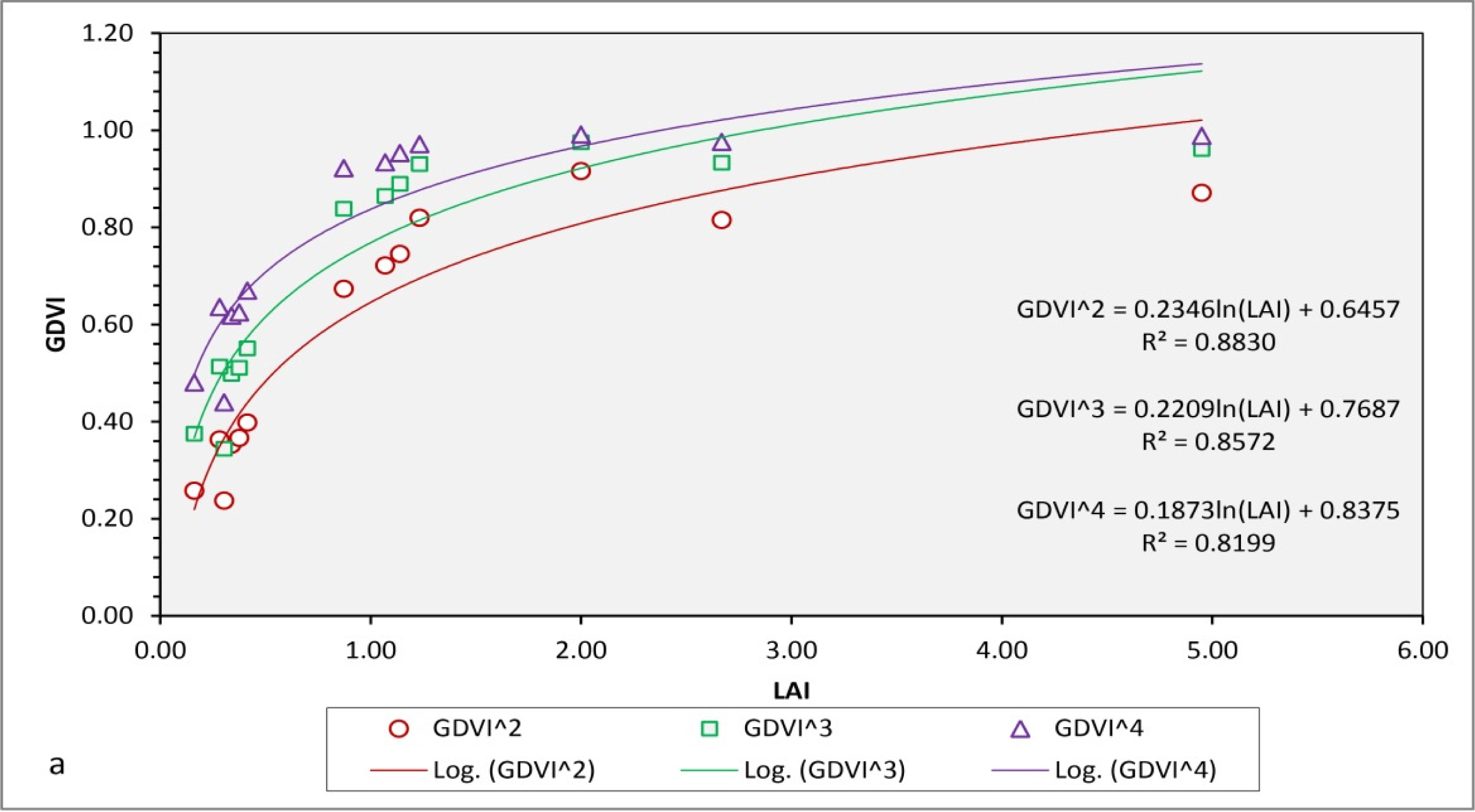
| 1 May 2007 | NDVI = 0.1784ln(LAI) + 0.4071 | 0.8729 |
| GDVI^2 = 0.2346ln(LAI) + 0.6457 | 0.8830 | |
| GDVI^3 = 0.2209ln(LAI) + 0.7687 | 0.8572 | |
| GDVI^4 = 0.1873ln(LAI) + 0.8375 | 0.8199 | |
| EVI = 0.1492ln(LAI) + 0.3528 | 0.7410 | |
| SAVI = 0.0935ln(LAI) + 0.2514 | 0.7302 | |
| SARVI = 0.1623ln(LAI) + 0.2574 | 0.8521 | |
| 21 August 2007 | NDVI = 0.1939ln(LAI) + 0.4185 | 0.9307 |
| GDVI^2 = 0.2737ln(LAI) + 0.6587 | 0.9547 | |
| GDVI^3 = 0.2812ln(LAI) + 0.7768 | 0.9432 | |
| GDVI^4 = 0.2619ln(LAI) + 0.8404 | 0.9135 | |
| EVI = 0.1729ln(LAI) + 0.374 | 0.7707 | |
| SAVI = 0.1118ln(LAI) + 0.2627 | 0.8000 | |
| SARVI = 0.1865ln(LAI) + 0.2729 | 0.8938 | |
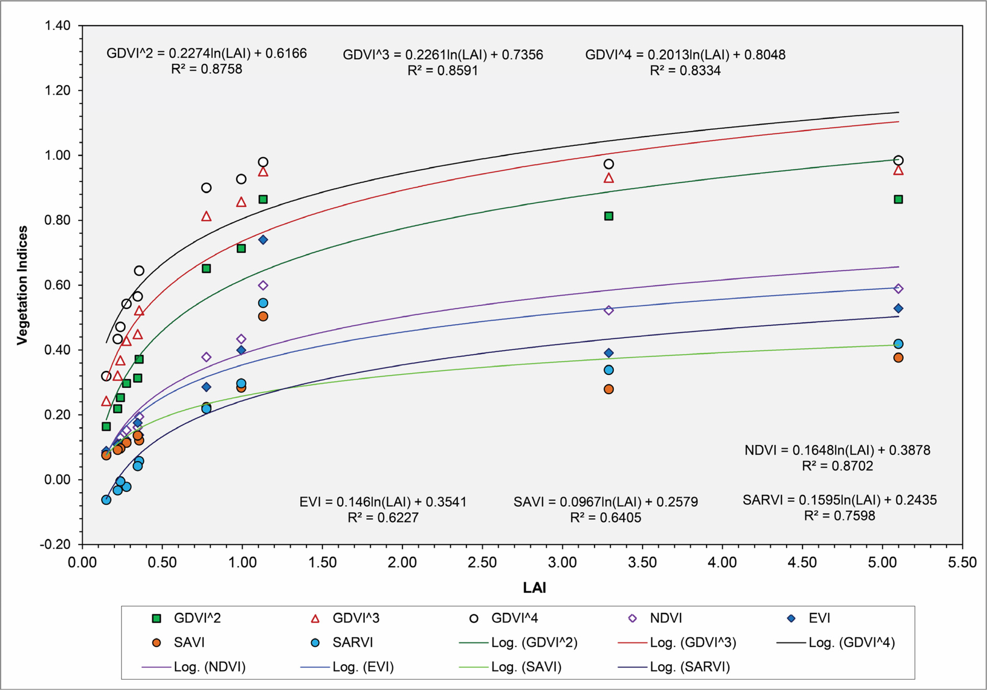
| 12 July 2010 | NDVI = 0.1648ln(LAI) + 0.3878 | 0.8702 |
| GDVI^2 = 0.2274ln(LAI) + 0.6166 | 0.8758 | |
| GDVI^3 = 0.2261ln(LAI) + 0.7356 | 0.8591 | |
| GDVI^4 = 0.2013ln(LAI) + 0.8048 | 0.8334 | |
| EVI = 0.146ln(LAI) + 0.3541 | 0.6227 | |
| SAVI = 0.0967ln(LAI) + 0.2579 | 0.6405 | |
| SARVI = 0.1595ln(LAI) + 0.2435 | 0.7598 | |
| 29 August 2010 | NDVI = 0.1761ln(LAI) + 0.3955 | 0.8983 |
| GDVI^2 = 0.248ln(LAI) + 0.6268 | 0.9319 | |
| GDVI^3 = 0.2538ln(LAI) + 0.7454 | 0.9255 | |
| GDVI^4 = 0.2338ln(LAI) + 0.8105 | 0.8921 | |
| EVI = 0.1527ln(LAI) + 0.3459 | 0.7365 | |
| SAVI = 0.0989ln(LAI) + 0.2469 | 0.7568 | |
| SARVI = 0.1698ln(LAI) + 0.2461 | 0.8656 | |
| VIs | Forest | Woodland | Citrus | Wheat | Barley | Olives | Grassland | Range-Land | Bare Land |
|---|---|---|---|---|---|---|---|---|---|
| GDVI^2 | 0.815 | 0.745 | 0.819 | 0.916 | 0.721 | 0.398 | 0.674 | 0.366 | 0.257 |
| GDVI^3 | 0.933 | 0.890 | 0.930 | 0.975 | 0.865 | 0.550 | 0.838 | 0.511 | 0.375 |
| GDVI^4 | 0.976 | 0.953 | 0.971 | 0.991 | 0.933 | 0.670 | 0.922 | 0.624 | 0.480 |
| NDVI | 0.522 | 0.453 | 0.536 | 0.678 | 0.440 | 0.212 | 0.390 | 0.193 | 0.131 |
| EVI | 0.399 | 0.353 | 0.512 | 0.674 | 0.349 | 0.145 | 0.337 | 0.169 | 0.120 |
| SAVI | 0.267 | 0.254 | 0.341 | 0.457 | 0.268 | 0.120 | 0.246 | 0.134 | 0.109 |
| SARVI | 0.350 | 0.292 | 0.395 | 0.521 | 0.273 | 0.093 | 0.255 | 0.072 | −0.023 |
| OSAVI | 0.322 | 0.295 | 0.373 | 0.487 | 0.300 | 0.138 | 0.271 | 0.141 | 0.104 |
| NLI | −0.227 | −0.262 | −0.025 | 0.282 | −0.214 | −0.557 | −0.266 | −0.434 | −0.370 |
| MNLI | −0.041 | −0.060 | −0.006 | 0.094 | −0.058 | −0.143 | −0.080 | −0.175 | −0.208 |
| WDRVI (a =0.20) | −0.216 | −0.302 | −0.191 | 0.042 | −0.307 | −0.526 | −0.372 | −0.541 | −0.587 |
| SARVI | SAVI | OSAVI | EVI | NLI | MNLI | NDVI | WDRVI | GDVI^2 | GDVI^3 | GDVI^4 | |
|---|---|---|---|---|---|---|---|---|---|---|---|
| FVC | 0.9663 | 0.9120 | 0.9821 | 0.9428 | 0.8172 | 0.9526 | 0.9683 | 0.9781 | 0.9683 | 0.9044 | 0.8336 |
| ln(FVC) | 0.7674 | 0.6496 | 0.7465 | 0.6626 | 0.4543 | 0.7500 | 0.8761 | 0.6773 | 0.8761 | 0.9332 | 0.9624 |
| exp(FVC) | 0.9624 | 0.9370 | 0.9841 | 0.9663 | 0.8686 | 0.9624 | 0.9197 | 0.9980 | 0.9197 | 0.8336 | 0.7534 |
| GDVI | Land Cover Types | ||||||||
|---|---|---|---|---|---|---|---|---|---|
| Forest/Maquis | Irrigated Cropland | Wood-Lands | Citrus/Orchard | Rainfed Cropland | Olive Plantation | Rangeland | Desert | Bare Land | |
| GDVI^2 | Partly, Yes | Partly, Yes | Yes | Yes | Yes | Yes | Yes | Yes | Yes |
| GDVI^3 | No | No | Yes | Yes | Yes | Yes | Yes | Yes | Yes |
| GDVI^4 | No | No | Partly, Yes | Partly, Yes | Partly, Yes | Yes | Yes | Yes | Yes |
© 2014 by the authors; licensee MDPI, Basel, Switzerland This article is an open access article distributed under the terms and conditions of the Creative Commons Attribution license (http://creativecommons.org/licenses/by/3.0/).
Share and Cite
Wu, W. The Generalized Difference Vegetation Index (GDVI) for Dryland Characterization. Remote Sens. 2014, 6, 1211-1233. https://0-doi-org.brum.beds.ac.uk/10.3390/rs6021211
Wu W. The Generalized Difference Vegetation Index (GDVI) for Dryland Characterization. Remote Sensing. 2014; 6(2):1211-1233. https://0-doi-org.brum.beds.ac.uk/10.3390/rs6021211
Chicago/Turabian StyleWu, Weicheng. 2014. "The Generalized Difference Vegetation Index (GDVI) for Dryland Characterization" Remote Sensing 6, no. 2: 1211-1233. https://0-doi-org.brum.beds.ac.uk/10.3390/rs6021211