Retrieval of Gap Fraction and Effective Plant Area Index from Phase-Shift Terrestrial Laser Scans

Abstract
:1. Introduction
2. Materials and Methods
2.1. Study Site
2.2. Data Acquisition and Scanner Characteristics
2.3. Scan Data Pre-Processing
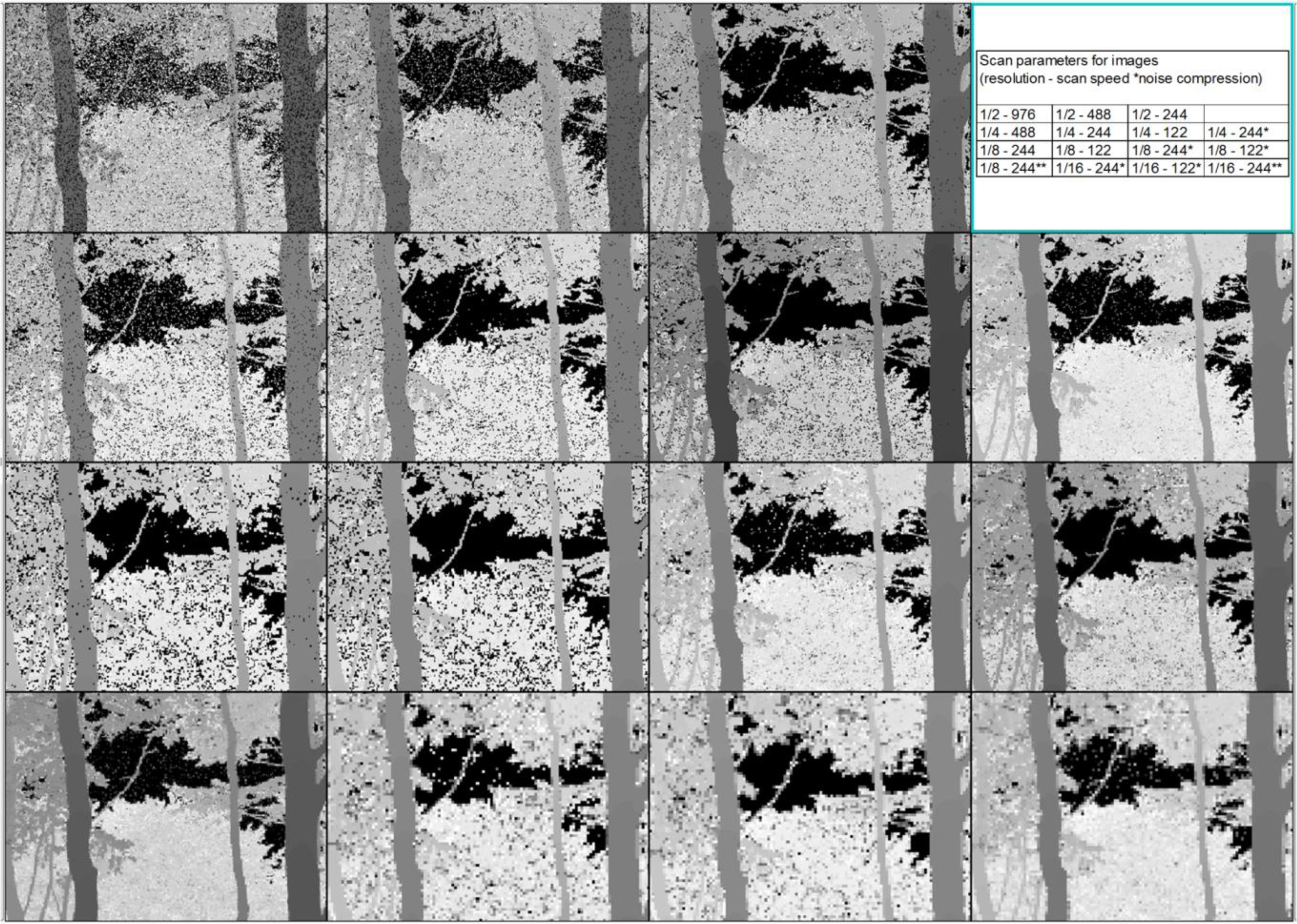
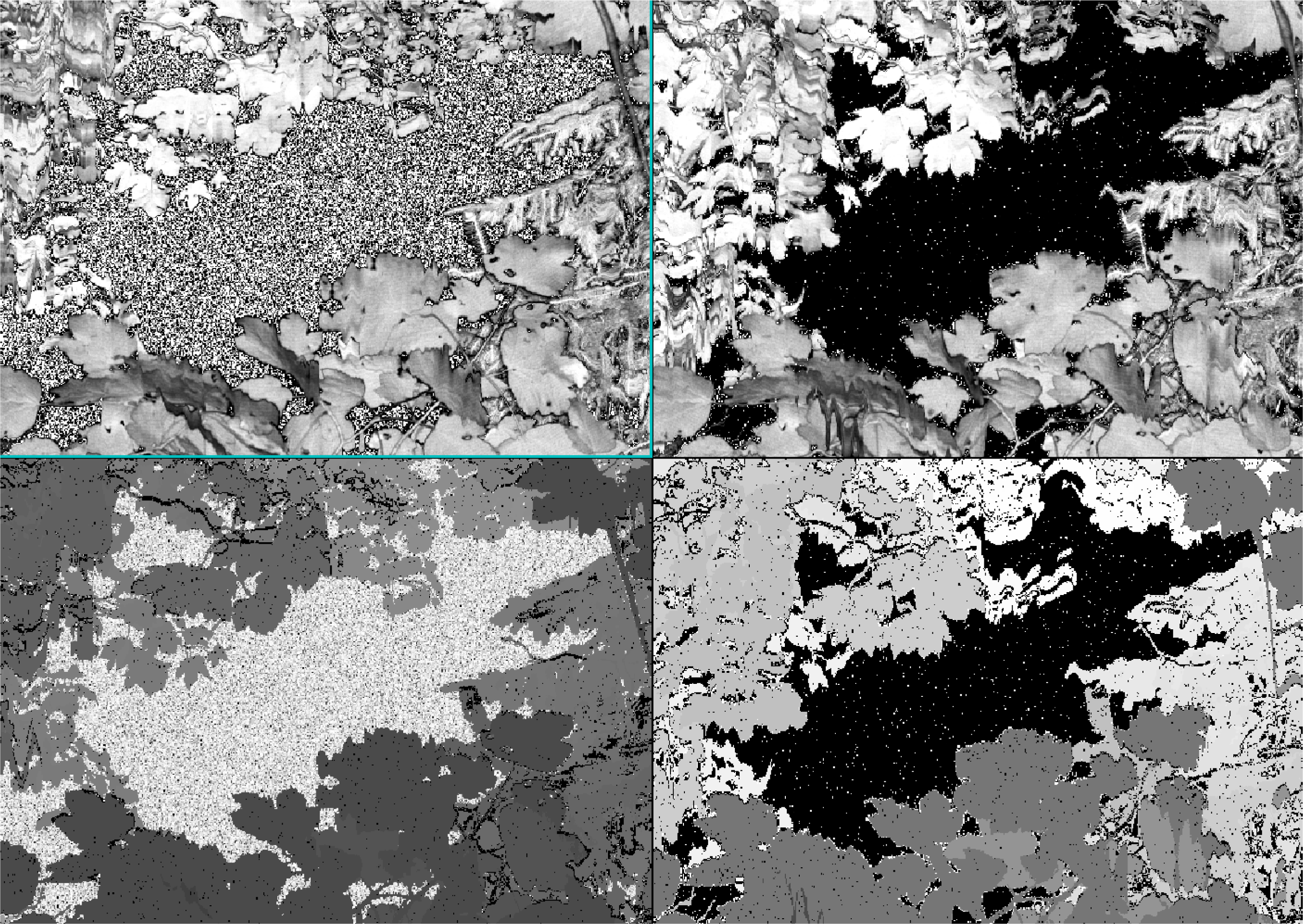
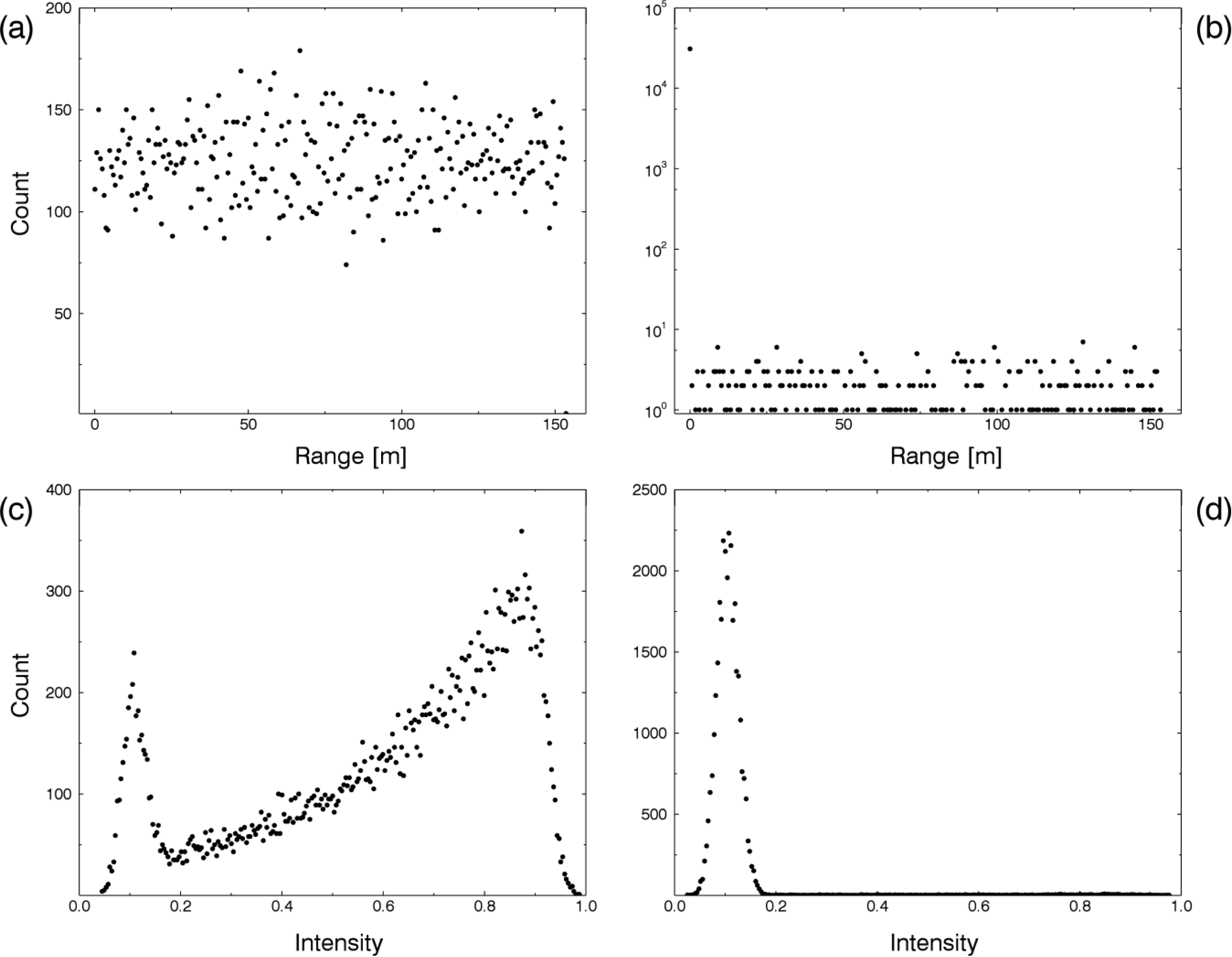
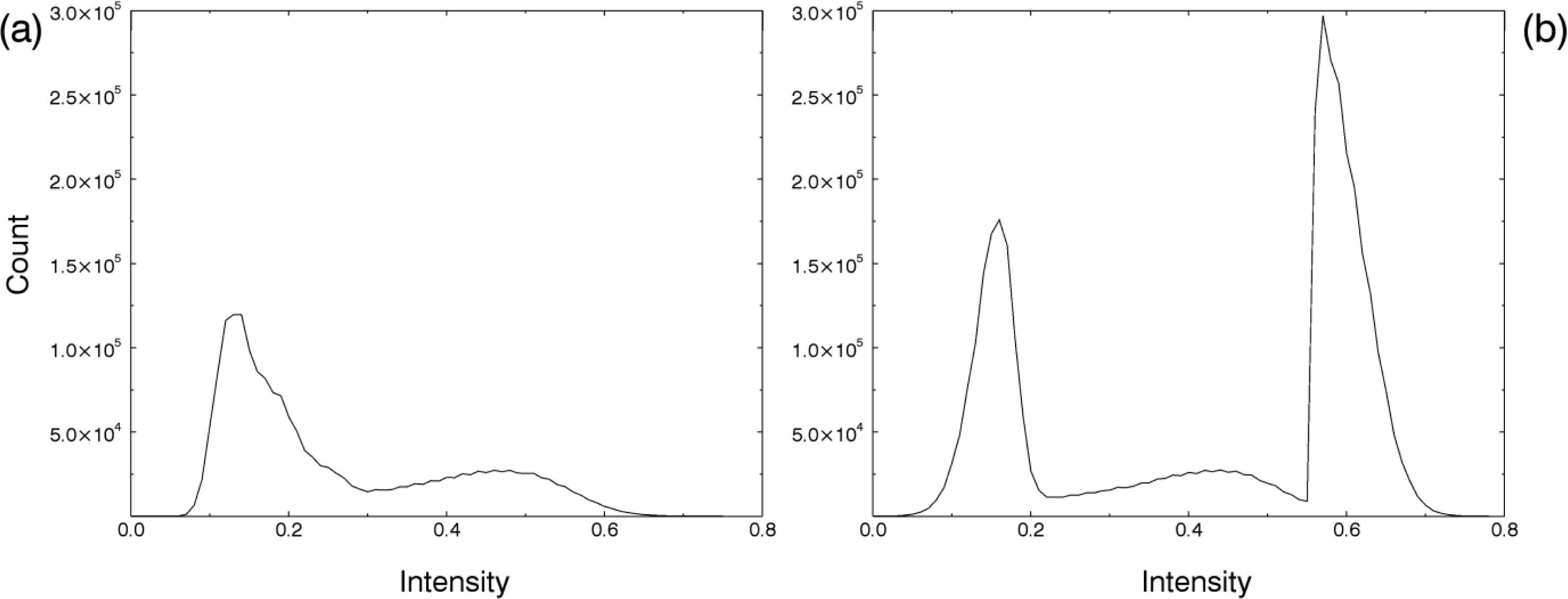
2.4. Scan Data Filtering
2.5. Gap Fraction and PAIe Calculation
3. Results and Discussion
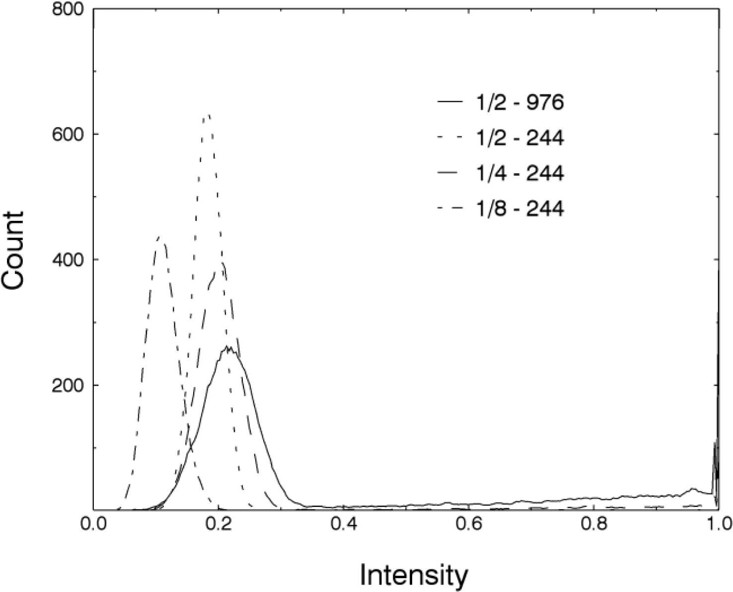
3.1. Data Filtering
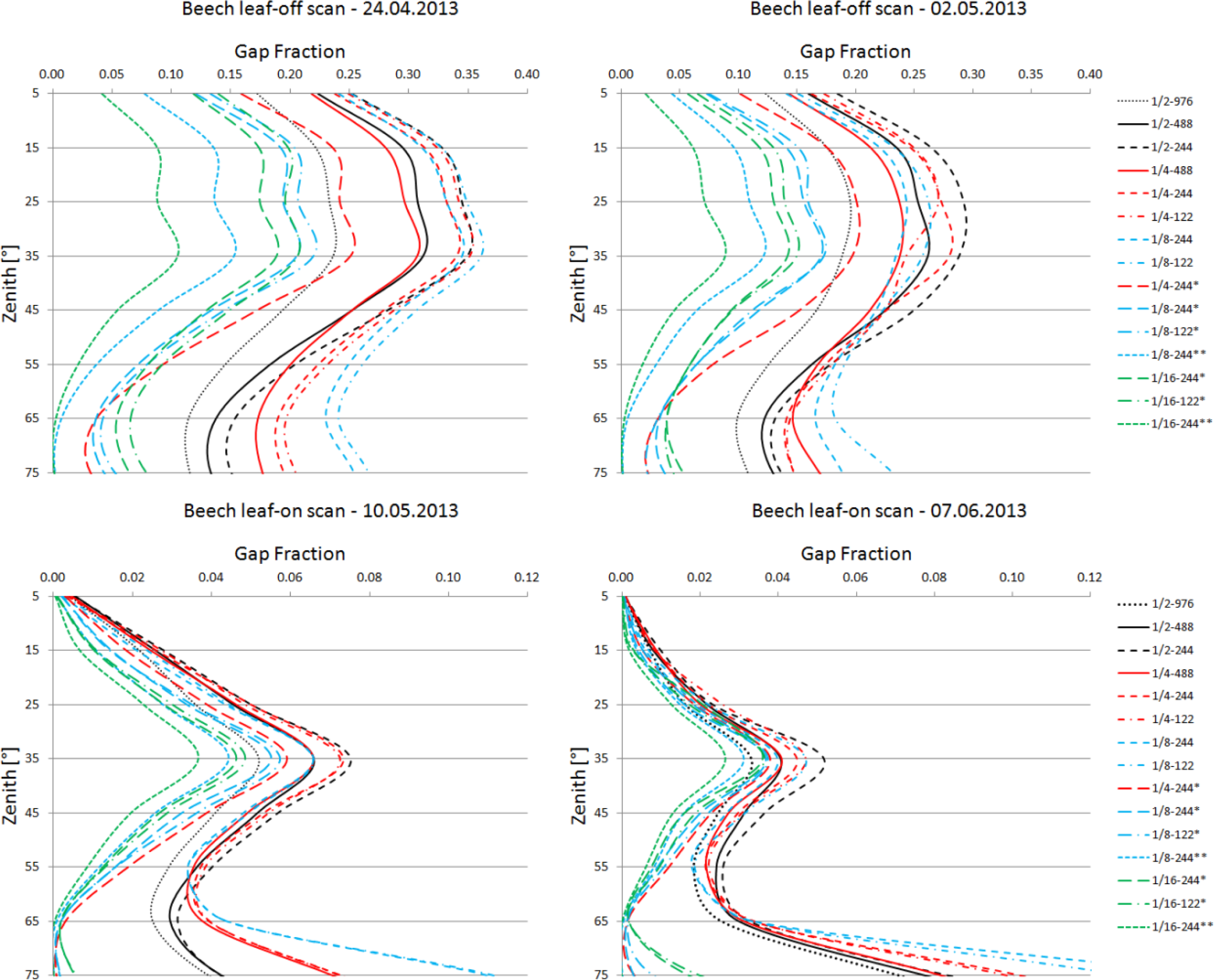
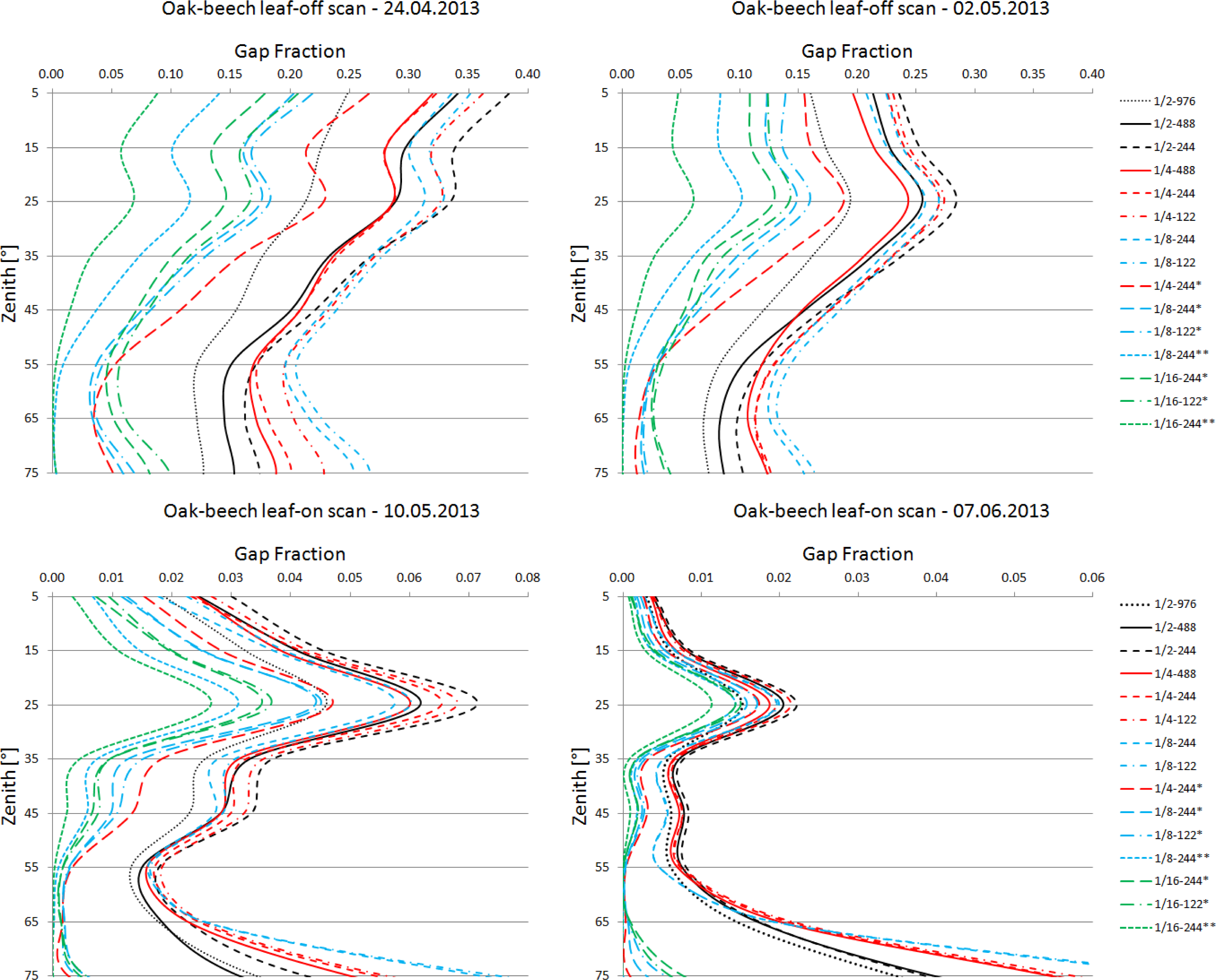
3.2. Gap Fraction
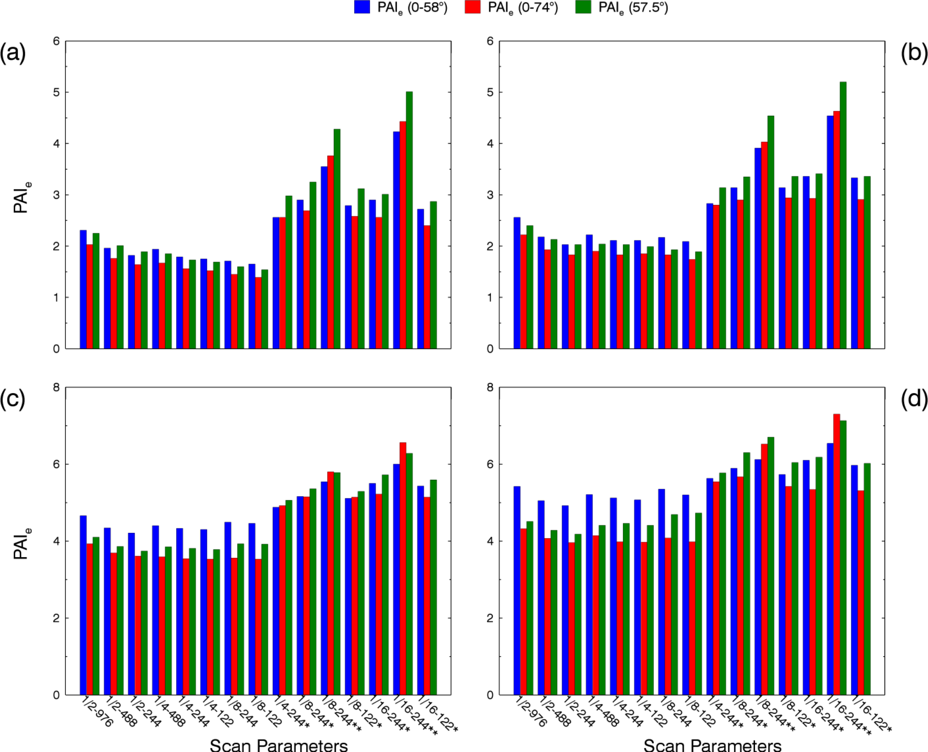
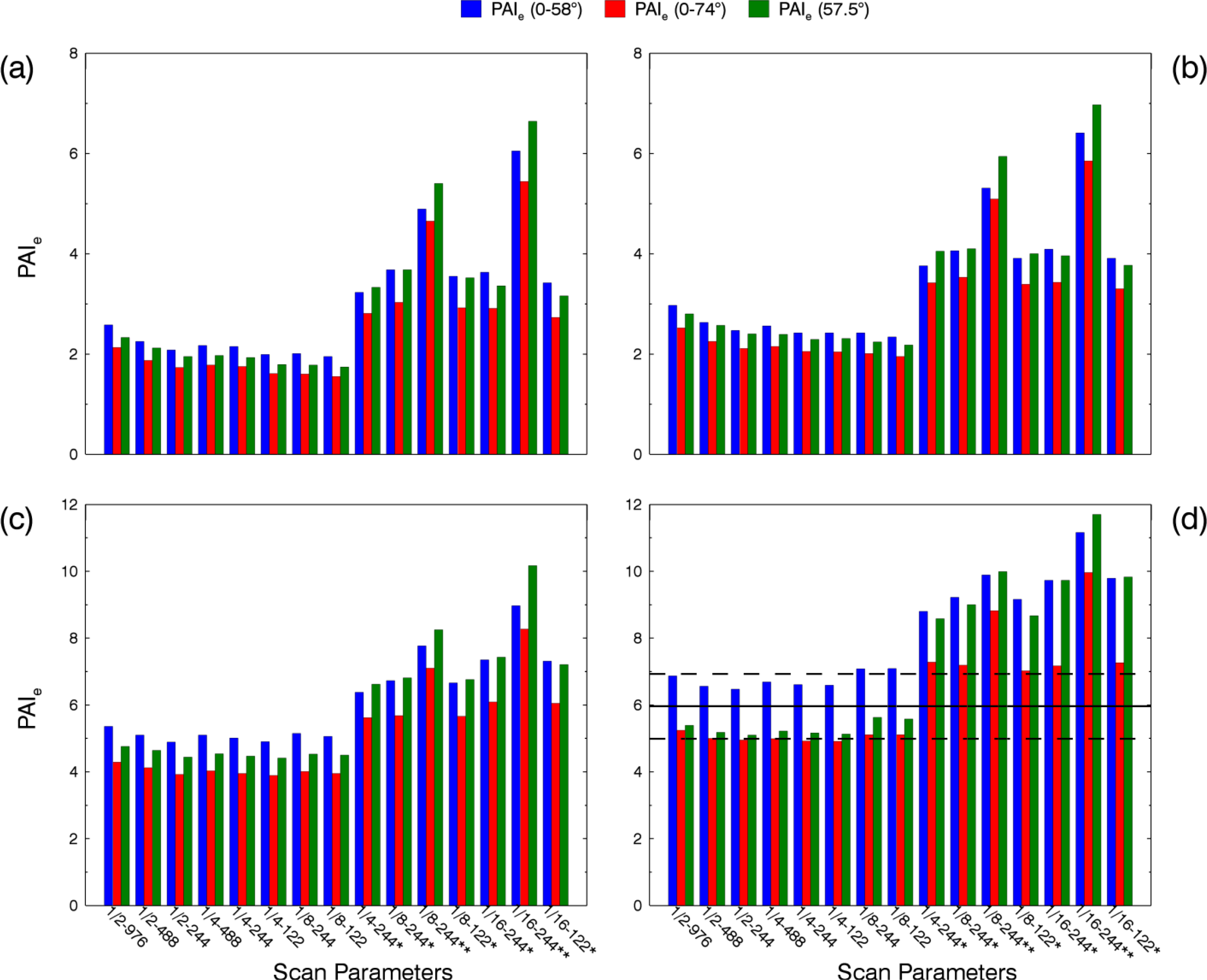
3.3. PAIe
3.4. Majority Filtering
3.5. Threshold Variation
4. Conclusions
Acknowledgments
Author Contributions
Conflicts of Interest
References
- Parker, G.G. Structure and Microclimate of Forest Canopies. In Forest Canopies: A Review of Research on a Biological Frontier; Lowman, M., Nadkarni, N., Eds.; Academic Press: San Diego, CA, USA, 1995; pp. 73–106. [Google Scholar]
- Chen, J.M.; Black, T.A. Defining leaf area index for non-flat leaves. Plant Cell Environ 1992, 15, 421–429. [Google Scholar]
- Jupp, D.L.B.; Culvenor, D.S.; Lovell, J.L.; Newnham, G.J.; Strahler, A.H.; Woodcock, C.E. Estimating forest LAI profiles and structural parameters using a ground-based laser called Echidna®. Tree Physiol 2008, 29, 171–181. [Google Scholar]
- Jonckheere, I.; Fleck, S.; Nackaerts, K.; Muys, B.; Coppin, P.; Weiss, M.; Baret, F. Review of methods for in situ leaf area index determination: Part I. Theories, sensors and hemispherical photography. Agric. For. Meteorol 2004, 121, 19–35. [Google Scholar]
- Warren Wilson, J. Inclined point quadrats. New Phytol 1960, 59, 1–8. [Google Scholar]
- Seidel, D. Terrestrial Laser Scanning: Applications in Forest Ecological Research. PhD Thesis, Georg-August Universität, Göttingen, Germany. 2011. [Google Scholar]
- Zheng, G.; Moskal, L.M. Retrieving leaf area index (LAI) using remote sensing: Theories, methods and sensors. Sensors 2009, 9, 2719–2745. [Google Scholar]
- Weiss, M.; Baret, F.; Smith, G.J.; Jonckheere, I.; Coppin, P. Review of methods for in situ leaf area index (LAI) determination: Part II. Estimation of LAI, errors and sampling. Agric. For. Meteorol 2004, 121, 37–53. [Google Scholar]
- Strahler, A.H.; Jupp, D.L.B.; Woodcock, C.E.; Schaaf, C.B.; Yao, T.; Zhao, F.; Yang, X.; Lovell, J.; Culvenor, D.; Newnham, G. Retrieval of forest structural parameters using a ground-based lidar instrument (Echidna®). Can. J. Remote Sens 2008, 34, S426–S440. [Google Scholar]
- Guang, Z.; Moskal, L.M.; Soo-Hyung, K. Retrieval of effective leaf area index in heterogeneous forests with terrestrial laser scanning. IEEE Trans. Geosci. Remote Sens 2013, 51, 777–786. [Google Scholar]
- Ramirez, F.; Armitage, R.; Danson, F. Testing the application of terrestrial laser scanning to measure forest canopy gap fraction. Remote Sens 2013, 5, 3037–3056. [Google Scholar]
- Zhao, F.; Yang, X.; Schull, M.A.; Román-Colón, M.O.; Yao, T.; Wang, Z.; Zhang, Q.; Jupp, D.L.B.; Lovell, J.L.; Culvenor, D.S. Measuring effective leaf area index, foliage profile, and stand height in New England forest stands using a full-waveform ground-based lidar. Remote Sens. Environ 2011, 115, 2954–2964. [Google Scholar]
- Dassot, M.; Constant, T.; Fournier, M. The use of terrestrial lidar technology in forest science: Application fields, benefits and challenges. Ann. For. Sci 2011, 68, 959–974. [Google Scholar]
- Newnham, G.; Armston, J.; Muir, J.; Goodwin, N.; Tindall, D.; Culvenor, D.; Püschel, P.; Nyström, M.; Johansen, K. Evaluation of Terrestrial Laser Scanners for Measuring Vegetation Structure: A Comparison of the Faro Focus 3D 120, Leica C10, Leica HDS7000 and Riegl VZ100a; CSIRO: Melbourne, Australia, 2012. [Google Scholar]
- Van Genechten, B. Theory and Practice on Terrestrial Laser Scanning: Training Material Based on Practical Applications; Santana Quintero, M., Lerma, J.L., Heine, E., van Genechten, B., Eds.; Universidad Politecnica de Valencia Editorial: Valencia, Spain, 2008. [Google Scholar]
- Simonse, M.; Aschoff, T.; Spiecker, H.; Thies, M. Automatic Determination of Forest Inventory Parameters Using Terrestrial Laserscanning. Proceedings of the ScandLaser Scientific Workshop on Airborne Laser Scanning of Forests, Umea, Sweden, 3–4 September 2003.
- Aschoff, T.; Spiecker, H. Algorithms for the automatic detection of trees in laser scanner data. Int. Arch. Photogramm. Remote Sens. Spat. Inf. Sci 66–70.
- Maas, H.G.; Bienert, A.; Scheller, S.; Keane, E. Automatic forest inventory parameter determination from terrestrial laser scanner data. Int. J. Remote Sens 2008, 29, 1579–1593. [Google Scholar]
- Antonarakis, A.S. Evaluating forest biometrics obtained from ground lidar in complex riparian forests. Remote Sens. Lett 2011, 2, 61–70. [Google Scholar]
- Bienert, A.; Scheller, S.; Keane, E.; Mullooly, G.; Mohan, F. Application of Terrestrial Laser Scanners for the Determination of Forest Inventory Parameters. Proceedings of the ISPRS Commission V Symposium “Image Engineering and Vision Metrology”, Dresden, Germany, 25–27 September 2006.
- Lovell, J.L.; Jupp, D.L.B.; Newnham, G.J.; Culvenor, D.S. Measuring tree stem diameters using intensity profiles from ground-based scanning lidar from a fixed viewpoint. ISPRS J. Photogramm. Remote Sens 2011, 66, 46–55. [Google Scholar]
- Tansey, K.; Selmes, N.; Anstee, A.; Tate, N.J.; Denniss, A. Estimating tree and stand variables in a Corsican pine woodland from terrestrial laser scanner data. Int. J. Remote Sens 2009, 30, 5195–5209. [Google Scholar]
- Pueschel, P.; Newnham, G.; Rock, G.; Udelhoven, T.; Werner, W.; Hill, J. The influence of scan mode and circle fitting on tree stem detection, stem diameter and volume extraction from terrestrial laser scans. ISPRS J. Photogramm. Remote Sens 2013, 77, 44–56. [Google Scholar]
- Yao, T.; Yang, X.; Zhao, F.; Wang, Z.; Zhang, Q.; Jupp, D.; Lovell, J.; Culvenor, D.; Newnham, G.; Ni-Meister, W. Measuring forest structure and biomass in New England forest stands using Echidna ground-based lidar. Remote Sens. Environ 2011, 115, 2965–2974. [Google Scholar]
- Holopainen, M.; Vastaranta, M.; Kankare, V.; Räty, M.; Vaaja, M.; Liang, X.; Yu, X.; Hyyppä, J.; Hyyppä, H.; Viitala, R. Biomass Estimation of Individual Trees Using Stem and Crown Diameter TLS Measurements. Proceedings of the 2011 ISPRS Workshop Laser Scanning, Calgary, AB, Canada, 29–31 August 2011; XXXVIII-5/W12.
- Kankare, V.; Holopainen, M.; Vastaranta, M.; Puttonen, E.; Yu, X.; Hyyppä, J.; Vaaja, M.; Hyyppä, H.; Alho, P. Individual tree biomass estimation using terrestrial laser scanning. ISPRS J. Photogramm. Remote Sens 2013, 75, 64–75. [Google Scholar]
- Béland, M.; Baldocchi, D.D.; Widlowski, J.-L.; Fournier, R.A.; Verstraete, M.M. On seeing the wood from the leaves and the role of voxel size in determining leaf area distribution of forests with terrestrial lidar. Agric. For. Meteorol 2014, 184, 82–97. [Google Scholar]
- Eitel, J.U.H.; Vierling, L.A.; Long, D.S. Simultaneous measurements of plant structure and chlorophyll content in broadleaf saplings with a terrestrial laser scanner. Remote Sens. Environ 2010, 114, 2229–2237. [Google Scholar]
- Henning, J.G.; Radtke, P.J. Ground-based laser imaging for assessing three-dimensional forest canopy structure. Photogramm. Eng. Remote Sens 2006, 72, 1349–1358. [Google Scholar]
- Van der Zande, D.; Stuckens, J.; Verstraeten, W.W.; Muys, B.; Coppin, P. Assessment of light environment variability in broadleaved forest canopies using terrestrial laser scanning. Remote Sens 2010, 2, 1564–1574. [Google Scholar]
- Bittner, S.; Gayler, S.; Biernath, C.; Winkler, J.B.; Seifert, S.; Pretzsch, H.; Priesack, E. Evaluation of a ray-tracing canopy light model based on terrestrial laser scans. Can. J. Remote Sens 2012, 38, 619–628. [Google Scholar]
- Zhao, F.; Strahler, A.H.; Schaaf, C.L.; Yao, T.; Yang, X.; Wang, Z.; Schull, M.A.; Román, M.O.; Woodcock, C.E.; Olofsson, P. Measuring gap fraction, element clumping index and LAI in Sierra forest stands using a full-waveform ground-based lidar. Remote Sens. Environ 2012, 125, 73–79. [Google Scholar]
- Clawges, R.; Vierling, L.; Calhoon, M.; Toomey, M. Use of a ground-based scanning lidar for estimation of biophysical properties of western larch (larix occidentalis). Int. J. Remote Sens 2007, 28, 4331–4344. [Google Scholar]
- Yang, X.; Strahler, A.H.; Schaaf, C.B.; Jupp, D.L.B.; Yao, T.; Zhao, F.; Wang, Z.; Culvenor, D.S.; Newnham, G.J.; Lovell, J.L. Three-dimensional forest reconstruction and structural parameter retrievals using a terrestrial full-waveform lidar instrument (Echidna®). Remote Sens. Environ 2013, 135, 36–51. [Google Scholar]
- Moskal, L.M.; Zheng, G. Retrieving forest inventory variables with terrestrial laser scanning (TLS) in urban heterogeneous forest. Remote Sens 2011, 4, 1–20. [Google Scholar]
- Hosoi, F.; Omasa, K. Voxel-based 3-D modeling of individual trees for estimating leaf area density using high-resolution portable scanning lidar. IEEE Trans. Geosci. Remote Sens 2006, 44, 3610–3618. [Google Scholar]
- Côté, J.-F.; Widlowski, J.-L.; Fournier, R.A.; Verstraete, M.M. The structural and radiative consistency of three-dimensional tree reconstructions from terrestrial lidar. Remote Sens. Environ 2009, 113, 1067–1081. [Google Scholar]
- Huang, P.; Pretzsch, H. Using terrestrial laser scanner for estimating leaf areas of individual trees in a conifer forest. Trees 2010, 24, 609–619. [Google Scholar]
- Danson, F.; Armitage, R.; Bandugula, V.; Ramirez, F.; Tate, N.; Tansey, K.; Tegzes, T. Terrestrial Laser Scanners to Measure Forest Canopy Gap Fraction. Proceedings of the 8th SilviLaser, Edinburgh, Scotland, 17–19 September 2008.
- Danson, F.M.; Hetherington, D.; Morsdorf, F.; Koetz, B.; Allgower, B. Forest canopy gap fraction from terrestrial laser scanning. IEEE Geosci. Remote Sens. Lett 2007, 4, 157–160. [Google Scholar]
- Zheng, G.; Moskal, L.M. Spatial variability of terrestrial laser scanning based leaf area index. Int. J. Appl. Earth Obs. Geoinf 2012, 19, 226–237. [Google Scholar]
- Calders, K.; Verbesselt, J.; Bartholomeus, H.; Herold, M. Applying Terrestrial Lidar to Derive Gap Fraction Distribution Time Series During Bud Break. Proceedings of the SilviLaser 2011, 11th International LiDAR Forest Applications Conference, Hobart, Australia, 16–20 October 2011.
- FARO, Faro Laser Scanner Photon 20/120 User’s Manual; FARO: Korntal-Münchingen, Germany, 2010.
- Hilker, T.; Leeuwen, M.; Coops, N.; Wulder, M.; Newnham, G.; Jupp, D.B.; Culvenor, D. Comparing canopy metrics derived from terrestrial and airborne laser scanning in a Douglas-fir dominated forest stand. Trees 2010, 24, 819–832. [Google Scholar]
- Greve, M. Vergleich von Methoden zur Erhebung des Blattflächenindex in Wäldern (In German)/Comparison of Methods for the Estimation of Leaf Area Index in Forests. M.Sc. Thesis, University of Trier, Trier, Germany. 2010. [Google Scholar]
- Ross, J.K. The Radiation Regime and Architecture of Plant Stands; Junk Publishers: The Hague, The Netherlands, 1981; p. 391. [Google Scholar]
- Black, T.A.; Chen, J.-M.; Lee, X.; Sagar, R.M. Characteristics of shortwave and longwave irradiances under a Douglas-fir forest stand. Can. J. For. Res 1991, 21, 1020–1028. [Google Scholar]
- Miller, J.B. A formula for average foliage density. Aust. J. Bot 1967, 15, 141–144. [Google Scholar]
- LI-COR Inc, LAI-2000 Plant Canopy Analyzer. Instruction Manual; LICOR Inc: Lincoln, NE, USA, 1992.
- Chen, J.M.; Govind, A.; Sonnentag, O.; Zhang, Y.; Barr, A.; Amiro, B. Leaf area index measurements at Fluxnet-Canada forest sites. Agric. For. Meteorol 2006, 140, 257–268. [Google Scholar]
- Leblanc, S.G.; Chen, J.M. A practical scheme for correcting multiple scattering effects on optical LAI measurements. Agric. For. Meteorol 2001, 110, 125–139. [Google Scholar]
- Wilson, J.W. Analysis of the spatial distribution of foliage by two-dimensional point quadrats. New Phytol 1959, 58, 92–101. [Google Scholar]
- Newnham, G.; Mashford, J.; Püschel, P.; Armston, J.; Culvenor, D.; Siggins, A.; Nyström, M.; Goodwin, N.; Muir, J. Non-Parametric Point Classification for Phase-Shift Laser Scanning. Proceedings of the SilviLaser 2012, Vancouver, BC, Canada, 16–19 September 2012.
- Pueschel, P. The influence of scanner parameters on the extraction of tree metrics from faro photon 120 terrestrial laser scans. ISPRS J. Photogramm. Remote Sens 2013, 78, 58–68. [Google Scholar]


| Resolution | Angular Step Size (°) | Point Spacing (cm/10 m) | Scan Speed (kpt/s) | Noise Compression | Scanning Time (min) | Filtering Time (min) |
|---|---|---|---|---|---|---|
| 1/2 | 0.018 | 0.3 | 976 | - | 03:24 | 03:25 |
| 488 | - | 06:49 | 03:15 | |||
| 244 | - | 13:39 | 02:30 | |||
| 1/4 | 0.036 | 0.6 | 488 | - | 01:42 | 01:06 |
| 244 | - | 03:24 | 01:01 | |||
| 122 | - | 06:49 | 01:01 | |||
| 244 | 2× | 13:39 | 16:02 | |||
| 1/8 | 0.072 | 1.3 | 244 | - | 00:51 | 00:30 |
| 122 | - | 01:42 | 00:26 | |||
| 244 | 2× | 03:24 | 04:16 | |||
| 122 | 2× | 06:49 | 04:18 | |||
| 244 | 4× | 13:39 | 14:20 | |||
| 1/16 | 0.144 | 2.5 | 244 | 2× | 00:51 | 01:15 |
| 122 | 2× | 01:42 | 01:10 | |||
| 244 | 4× | 03:24 | 03:45 | |||
| Leaf-Off | Leaf-On | ||||||
|---|---|---|---|---|---|---|---|
| Percentage Deviation (%) | Percentage Deviation (%) | ||||||
| Site | Parameters | PAIe (0–58°) | PAIe (0–74°) | PAIe (57.5°) | PAIe (0–58°) | PAIe (0–74°) | PAIe (57.5°) |
| Beech | 1/2—976 | −5.8 | −4.9 | −3.0 | −3.4 | −2.7 | −1.4 |
| 1/2—488 | −4.2 | −3.8 | −2.7 | −2.0 | −1.6 | −0.9 | |
| 1/2—244 | −1.5 | −1.8 | −1.7 | −0.4 | −0.4 | −0.3 | |
| 1/4—488 | −5.5 | −5.1 | −4.1 | −2.1 | −1.8 | −1.1 | |
| 1/4—244 | −3.7 | −3.6 | −3.6 | −0.7 | −0.7 | −0.6 | |
| 1/4—122 | −3.4 | −3.4 | −3.6 | −0.5 | −0.6 | −0.6 | |
| 1/8—244 | −7.8 | −7.2 | −7.1 | −1.4 | −1.6 | −1.5 | |
| 1/8—122 | −8.0 | −7.6 | −7.7 | −1.1 | −1.3 | −1.4 | |
| 1/4—244—2× | −1.4 | −1.1 | −0.8 | −0.8 | −0.5 | −0.6 | |
| 1/8—244—2× | −1.4 | −1.1 | −0.9 | −0.8 | −0.5 | −0.5 | |
| 1/8—244—4× | −2.6 | −1.7 | −1.2 | −2.1 | −1.3 | −1.1 | |
| 1/8—122—2× | −1.0 | −0.8 | −0.7 | −0.2 | −0.1 | −0.2 | |
| 1/16—244—2× | −1.8 | −1.5 | −0.7 | −0.8 | −0.5 | −0.7 | |
| 1/16—244—4× | −2.3 | −1.5 | −1.1 | −1.8 | −1.0 | −0.8 | |
| 1/16—122—2× | −1.6 | −1.4 | −0.8 | −0.3 | −0.2 | −0.5 | |
| Oak-beech | 1/2—976 | −4.3 | −4.2 | −2.5 | −1.6 | −1.6 | −0.6 |
| 1/2—488 | −3.6 | −3.5 | −2.6 | −1.0 | −1.0 | −0.4 | |
| 1/2—244 | −2.0 | −2.1 | −2.3 | −0.4 | −0.4 | −0.3 | |
| 1/4—488 | −5.1 | −4.9 | −4.0 | −1.4 | −1.4 | −0.9 | |
| 1/4—244 | −4.8 | −4.7 | −4.2 | −0.8 | −0.8 | −0.7 | |
| 1/4—122 | −3.9 | −3.9 | −4.0 | −0.8 | −0.7 | −0.7 | |
| 1/8—244 | −7.7 | −7.5 | −6.8 | −2.1 | −1.9 | −1.9 | |
| 1/8—122 | −7.8 | −7.6 | −7.1 | −2.0 | −1.9 | −2.0 | |
| 1/4—244—2× | −1.0 | −0.8 | −0.7 | −0.4 | −0.3 | −0.2 | |
| 1/8—244—2× | −0.9 | −0.8 | −0.5 | −0.3 | −0.3 | −0.1 | |
| 1/8—244—4× | −1.0 | −0.8 | −0.4 | −0.6 | −0.7 | 0.0 | |
| 1/8—122—2× | −0.9 | −0.7 | −0.6 | −0.1 | −0.2 | −0.1 | |
| 1/16—244—2× | −1.0 | −1.0 | −0.5 | −0.2 | −0.2 | 0.0 | |
| 1/16—244—4× | −0.6 | −0.7 | −0.2 | −0.3 | −0.3 | 0.0 | |
| 1/16—122—2× | −1.3 | −1.2 | −0.7 | −0.1 | −0.1 | 0.0 | |
| (a) | |||||||
|---|---|---|---|---|---|---|---|
| % Deviation (Decrease of Threshold by 5%) | % Deviation (Increase of Threshold by 5%) | ||||||
| Site | Parameters | PAIe (0–58°) | PAIe (0–74°) | PAIe (57.5°) | PAIe (0–58°) | PAIe (0–74°) | PAIe (57.5°) |
| Beech | 1/2—976 | 7.0 | 6.8 | 8.0 | −3.0 | −2.6 | −3.5 |
| 1/2—488 | 6.2 | 5.8 | 7.2 | −2.4 | −1.9 | −2.8 | |
| 1/2—244 | 8.5 | 6.9 | 7.3 | −3.0 | −2.0 | −2.6 | |
| 1/4—488 | 13.2 | 13.1 | 14.3 | −6.6 | −5.4 | −6.9 | |
| 1/4—244 | 11.8 | 10.3 | 12.7 | −5.6 | −4.3 | −6.1 | |
| 1/4—122 | 10.7 | 10.0 | 11.4 | −5.8 | −4.9 | −5.8 | |
| 1/8—244 | 16.1 | 15.6 | 22.1 | −10.8 | −9.1 | −12.2 | |
| 1/8—122 | 19.7 | 18.7 | 26.3 | −11.7 | −9.9 | −13.8 | |
| 1/4—244—2× | 4.0 | 2.4 | 2.9 | −0.9 | −0.5 | −0.4 | |
| 1/8—244—2× | 5.7 | 4.3 | 5.3 | −1.2 | −0.9 | −1.3 | |
| 1/8—244—4× | 2.6 | 1.9 | 1.6 | −0.5 | −0.2 | −0.2 | |
| 1/8—122—2× | 4.4 | 4.1 | 3.4 | −1.7 | −1.3 | −0.8 | |
| 1/16—244—2× | 10.7 | 10.9 | 11.0 | −4.2 | −3.5 | −4.0 | |
| 1/16—244—4× | 1.5 | 1.7 | 0.8 | −0.4 | −0.2 | −0.2 | |
| 1/16—122—2× | 7.5 | 7.8 | 9.6 | −4.6 | −3.3 | −4.2 | |
| Oak-beech | 1/2—976 | 10.8 | 9.5 | 9.1 | −4.3 | −3.7 | −3.9 |
| 1/2—488 | 10.3 | 8.6 | 8.9 | −3.7 | −3.1 | −3.3 | |
| 1/2—244 | 9.5 | 7.8 | 8.7 | −3.4 | −2.7 | −2.4 | |
| 1/4—488 | 14.4 | 12.0 | 13.2 | −6.6 | −5.5 | −6.0 | |
| 1/4—244 | 14.4 | 12.1 | 13.9 | −6.3 | −5.4 | −6.0 | |
| 1/4—122 | 10.8 | 9.1 | 11.4 | −5.4 | −4.8 | −5.2 | |
| 1/8—244 | 16.4 | 15.1 | 16.9 | −9.9 | −8.9 | −9.6 | |
| 1/8—122 | 18.4 | 16.9 | 18.7 | −10.5 | −9.5 | −10.1 | |
| 1/4—244—2× | 5.5 | 3.2 | 4.2 | −0.9 | −0.7 | −0.3 | |
| 1/8—244—2× | 3.9 | 3.2 | 3.6 | −1.3 | −1.2 | −1.1 | |
| 1/8—244—4× | 0.5 | 0.3 | 0.5 | −0.2 | −0.1 | 0.0 | |
| 1/8—122—2× | 3.1 | 2.4 | 3.4 | −1.0 | −0.9 | −1.0 | |
| 1/16—244—2× | 10.1 | 9.0 | 10.7 | −4.6 | −4.0 | −4.1 | |
| 1/16—244—4× | 1.4 | 0.6 | 1.8 | −0.2 | −0.1 | −0.2 | |
| 1/16—122—2× | 12.8 | 11.3 | 10.3 | −4.9 | −4.4 | −3.9 | |
| (b) | |||||||
|---|---|---|---|---|---|---|---|
| % Deviation (Decrease of Threshold by 5%) | % Deviation (Increase of Threshold by 5%) | ||||||
| Site | Parameters | PAIe (0–58°) | PAIe (0–74°) | PAIe (57.5°) | PAIe (0–58°) | PAIe (0–74°) | PAIe (57.5°) |
| Beech | 1/2—976 | 6.2 | 6.8 | 9.6 | −4.3 | −3.9 | −7.1 |
| 1/2—488 | 4.9 | 5.8 | 9.9 | −3.9 | −3.4 | −6.9 | |
| 1/2—244 | 5.7 | 6.2 | 10.4 | −4.0 | −3.2 | −7.0 | |
| 1/4—488 | 4.6 | 6.6 | 10.8 | −4.8 | −4.8 | −11.4 | |
| 1/4—244 | 5.2 | 7.9 | 12.1 | −5.1 | −5.1 | −12.4 | |
| 1/4—122 | 5.5 | 7.8 | 11.4 | −4.8 | −4.8 | −12.2 | |
| 1/8—244 | 6.8 | 11.5 | 12.8 | −6.0 | −6.9 | −16.1 | |
| 1/8—122 | 4.3 | 8.6 | 12.4 | −5.1 | −6.2 | −15.8 | |
| 1/4—244—2× | 0.6 | 1.0 | 0.4 | −0.2 | −0.4 | −0.4 | |
| 1/8—244—2× | 2.6 | 2.7 | 0.5 | −0.4 | −1.3 | −0.9 | |
| 1/8—244—4× | 0.7 | 0.8 | 3.0 | 0.0 | 0.0 | −0.1 | |
| 1/8—122—2× | 0.5 | 2.6 | 0.4 | −0.3 | −1.4 | −1.1 | |
| 1/16—244—2× | 3.5 | 6.7 | 1.2 | −1.3 | −2.8 | −1.7 | |
| 1/16—244—4× | 0.8 | 0.7 | 1.2 | 0.0 | 0.0 | 0.0 | |
| 1/16—122—2× | 0.8 | 5.4 | 1.2 | −0.5 | −2.5 | −2.1 | |
| Oak-beech | 1/2—976 | 6.9 | 6.3 | 8.5 | −4.8 | −4.1 | −6.3 |
| 1/2—488 | 5.4 | 4.8 | 7.9 | −4.3 | −3.6 | −6.0 | |
| 1/2—244 | 5.9 | 5.2 | 8.4 | −4.4 | −3.6 | −6.0 | |
| 1/4—488 | 7.9 | 7.6 | 11.4 | −6.8 | −6.1 | −9.3 | |
| 1/4—244 | 7.8 | 7.7 | 11.5 | −6.8 | −6.1 | −9.4 | |
| 1/4—122 | 7.6 | 7.5 | 12.1 | −6.7 | −6.0 | −9.5 | |
| 1/8—244 | 10.1 | 10.3 | 15.4 | −8.8 | −8.4 | −12.5 | |
| 1/8—122 | 10.7 | 11.0 | 16.6 | −9.1 | −8.6 | −12.5 | |
| 1/4—244—2× | 0.8 | 1.3 | 1.3 | −0.5 | −0.7 | −1.3 | |
| 1/8—244—2× | 1.5 | 2.6 | 3.5 | −1.1 | −1.7 | −3.3 | |
| 1/8—244—4× | 2.6 | 2.6 | 1.5 | 0.0 | 0.0 | 0.0 | |
| 1/8—122—2× | 1.6 | 2.8 | 3.7 | −1.3 | −1.7 | −3.0 | |
| 1/16—244—2× | 2.5 | 4.6 | 3.1 | −2.4 | −3.2 | −6.1 | |
| 1/16—244—4× | 0.4 | 0.2 | 0.0 | 0.0 | 0.0 | 0.0 | |
| 1/16—122—2× | 2.4 | 4.6 | 4.3 | −2.5 | −3.3 | −6.3 | |
© 2014 by the authors; licensee MDPI, Basel, Switzerland This article is an open access article distributed under the terms and conditions of the Creative Commons Attribution license (http://creativecommons.org/licenses/by/3.0/).
Share and Cite
Pueschel, P.; Newnham, G.; Hill, J. Retrieval of Gap Fraction and Effective Plant Area Index from Phase-Shift Terrestrial Laser Scans. Remote Sens. 2014, 6, 2601-2627. https://0-doi-org.brum.beds.ac.uk/10.3390/rs6032601
Pueschel P, Newnham G, Hill J. Retrieval of Gap Fraction and Effective Plant Area Index from Phase-Shift Terrestrial Laser Scans. Remote Sensing. 2014; 6(3):2601-2627. https://0-doi-org.brum.beds.ac.uk/10.3390/rs6032601
Chicago/Turabian StylePueschel, Pyare, Glenn Newnham, and Joachim Hill. 2014. "Retrieval of Gap Fraction and Effective Plant Area Index from Phase-Shift Terrestrial Laser Scans" Remote Sensing 6, no. 3: 2601-2627. https://0-doi-org.brum.beds.ac.uk/10.3390/rs6032601