A Combination of TsHARP and Thin Plate Spline Interpolation for Spatial Sharpening of Thermal Imagery


Abstract
:1. Introduction
2. Methodology
2.1. Notations and Definitions
| n: | the number of coarse pixels in low-resolution thermal imagery; |
| m: | the number of fine pixels covering the same area as a coarse pixel; |
| N: | the number of fine pixels in high-resolution VNIR imagery, which are equal to n × m; |
| (x, y): | row and column index of a certain pixel; |
| i: | index of a coarse pixel, i = 1, …, n; |
| j: | index of fine pixels in each coarse pixel, j = 1, …, m; |
| Thigh(xij, yij): | True LST at the fine pixel (xij, yij); |
| Tlow(xi, yi): | LST at the coarse pixel (xi, yi); |
| NDVIhigh(xij, yij): | NDVI at the fine pixel (xij, yij); |
| NDVIlow(xi, yi): | Aggregated NDVI at the coarse pixel (xi, yi). |
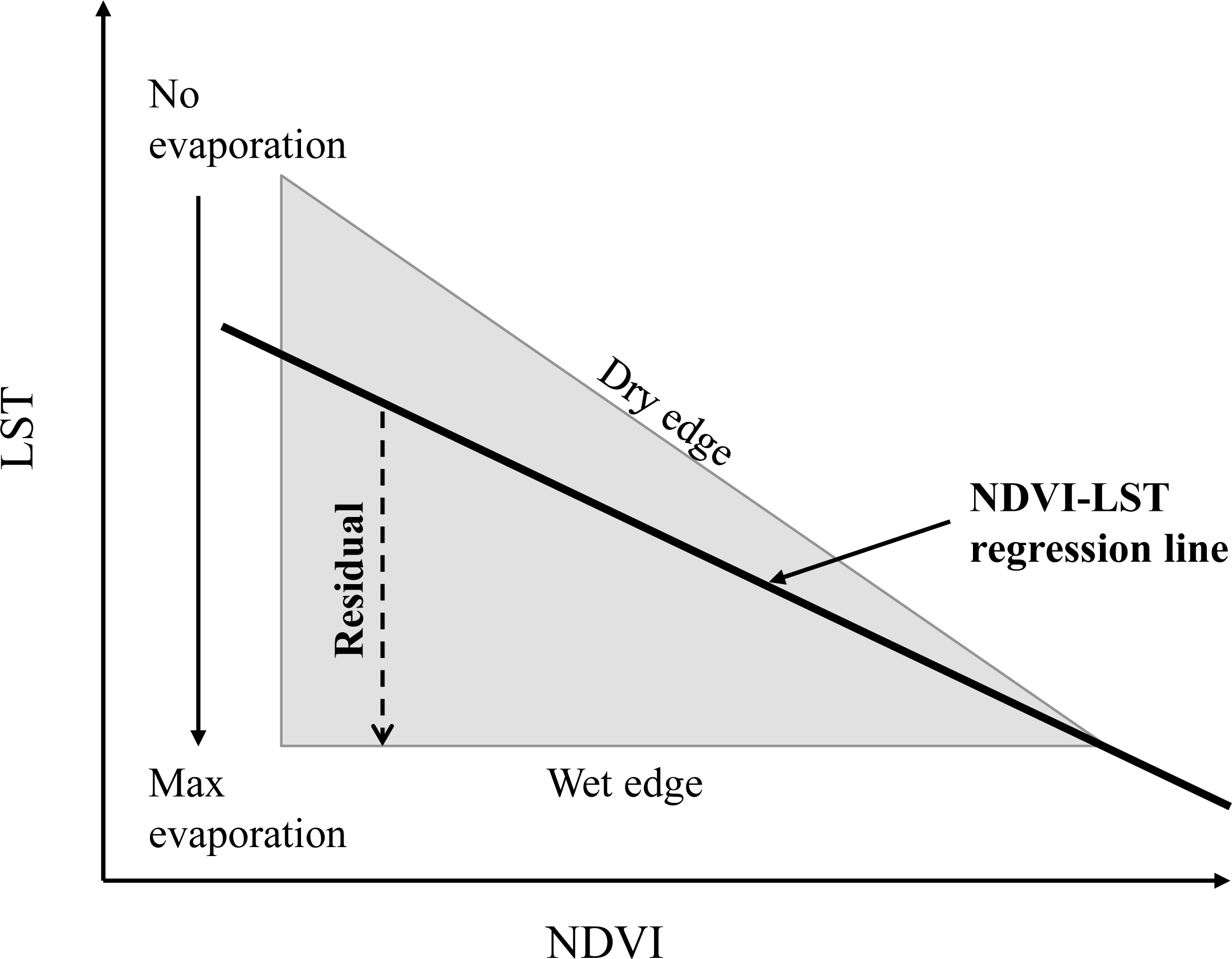
2.2. TsHARP Method
2.3. Thin Plate Spline (TPS) Interpolation
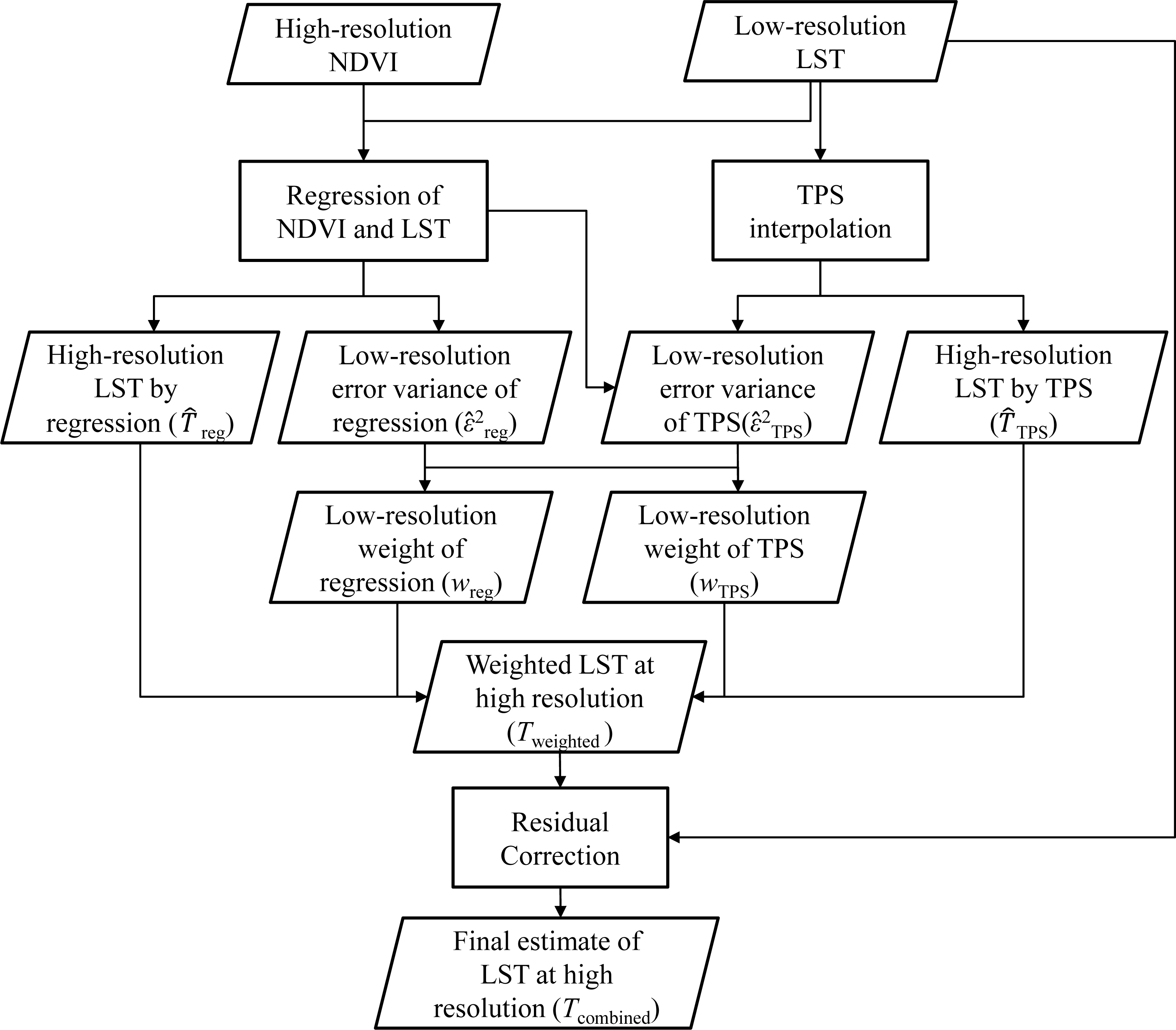
2.4. Combination of TsHARP and TPS
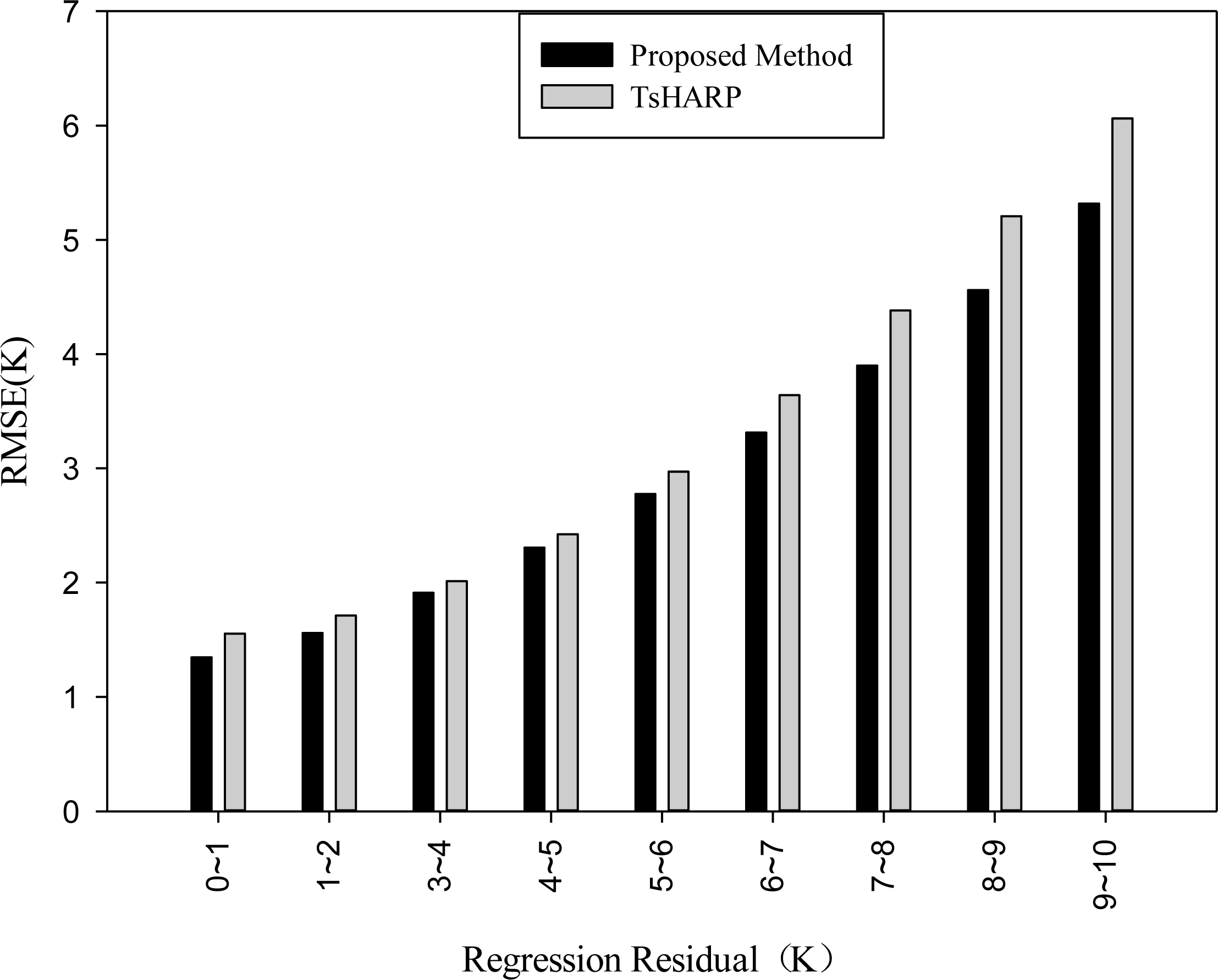
2.4.1. Error Estimation of the Regression Method
2.4.2. Error Estimation of TPS
2.4.3. Combination of TPS and Regression Method
3. Experiments
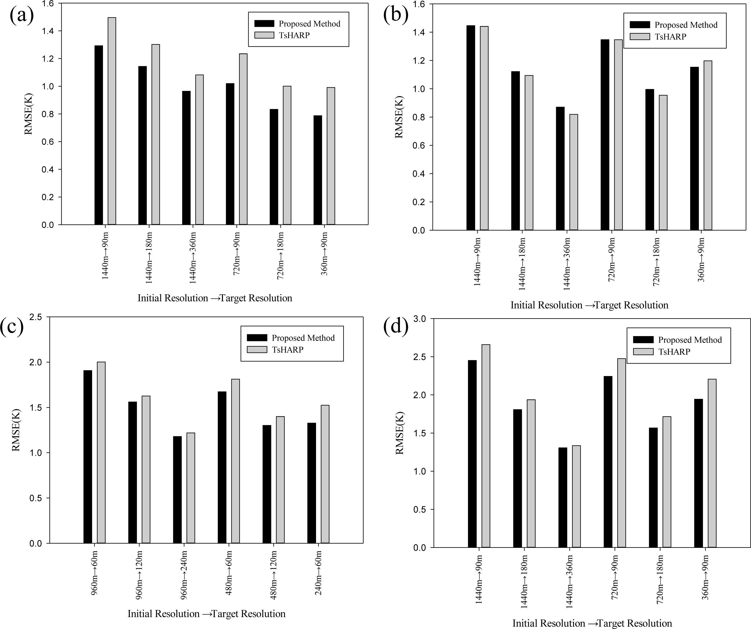
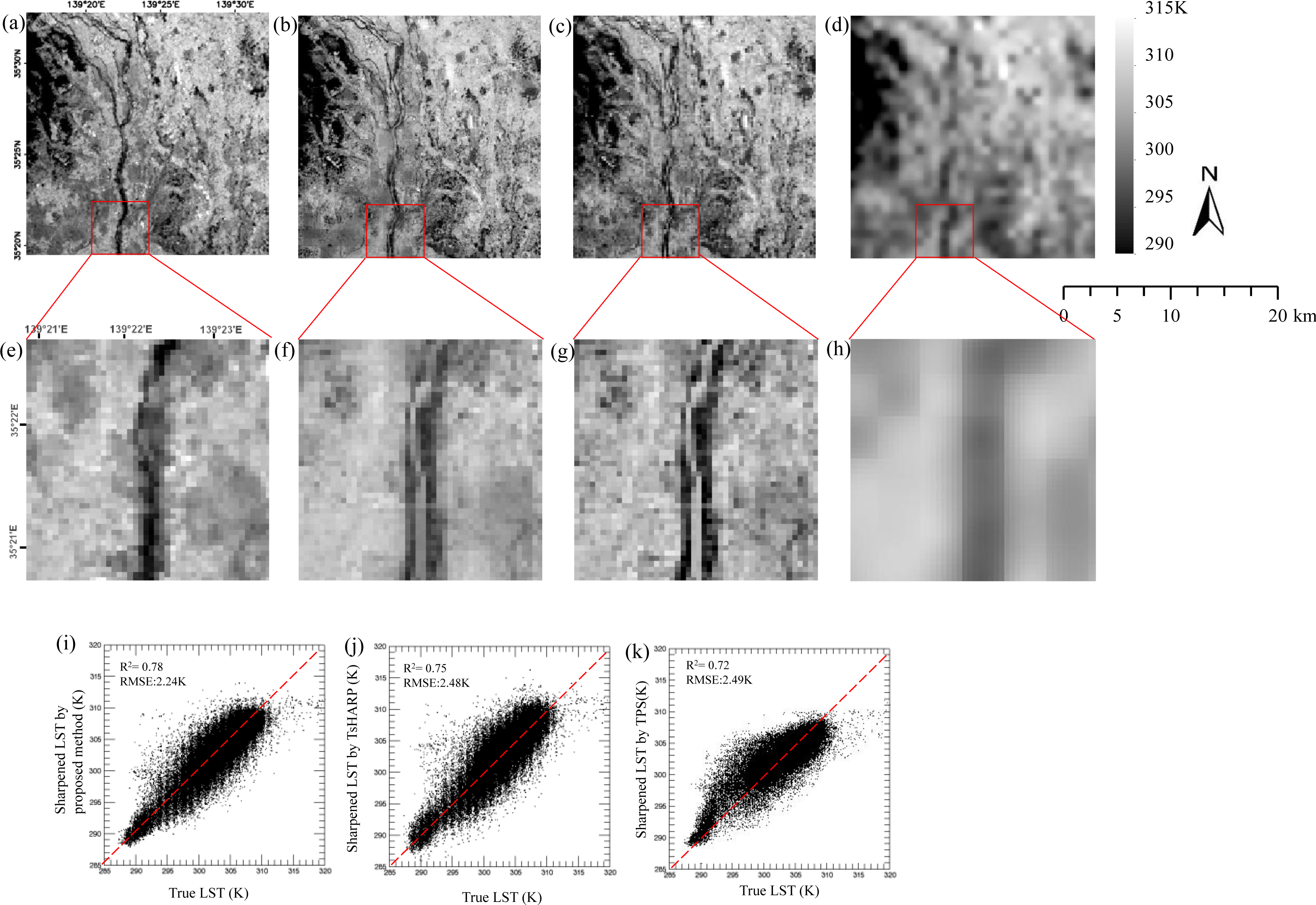
3.1. Simulation Experiment Using ASTER Data
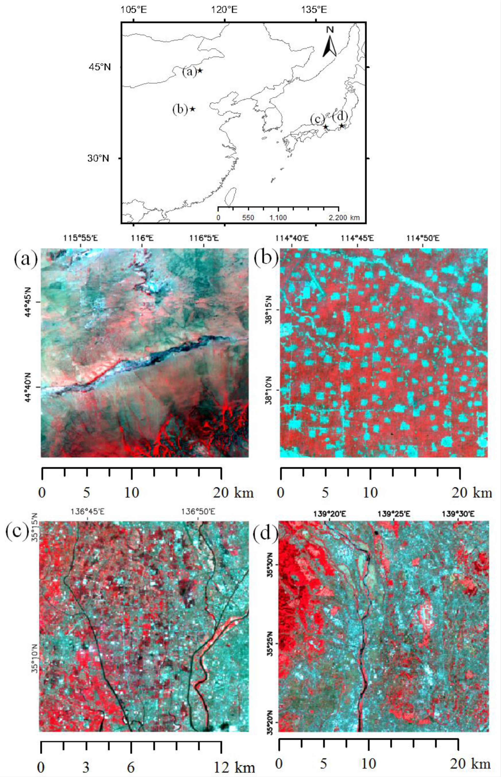
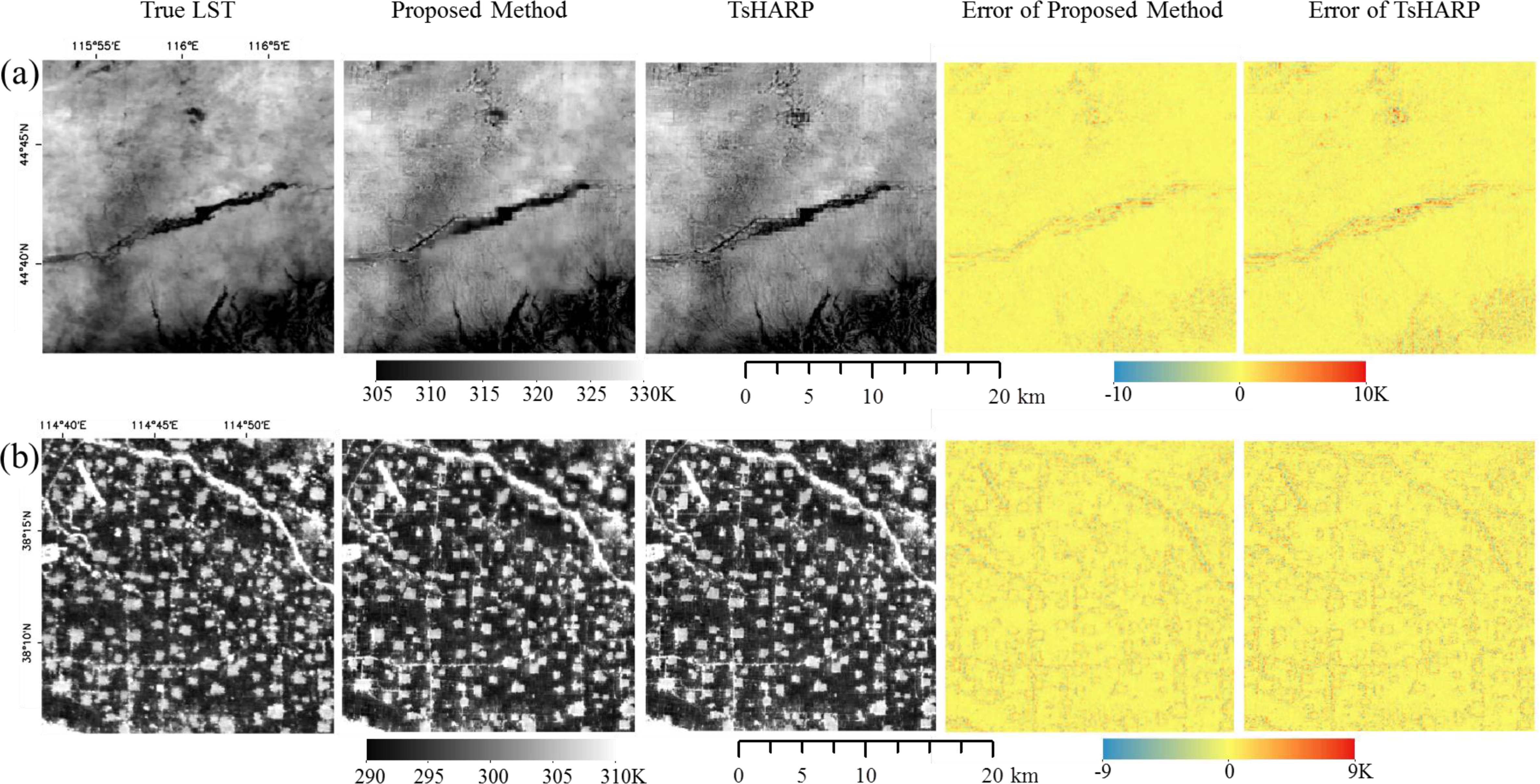
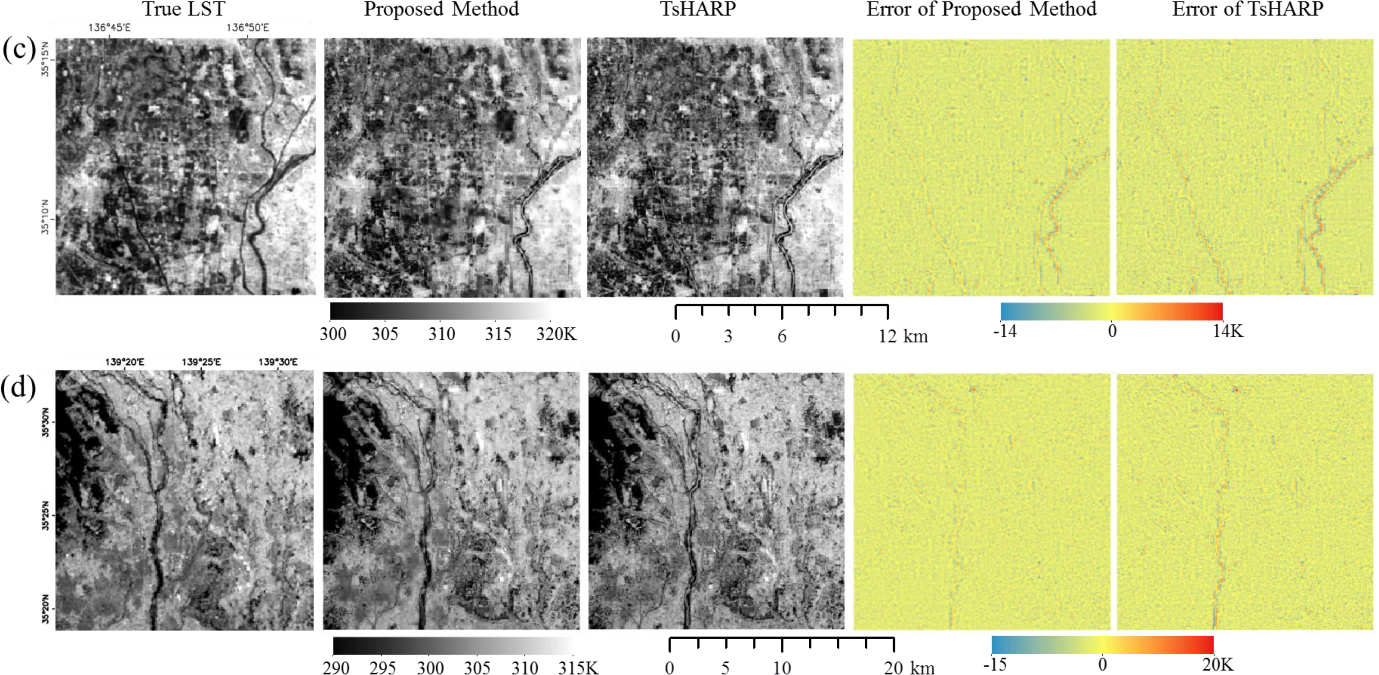
3.2. Simulation Experiments across Different Landscapes
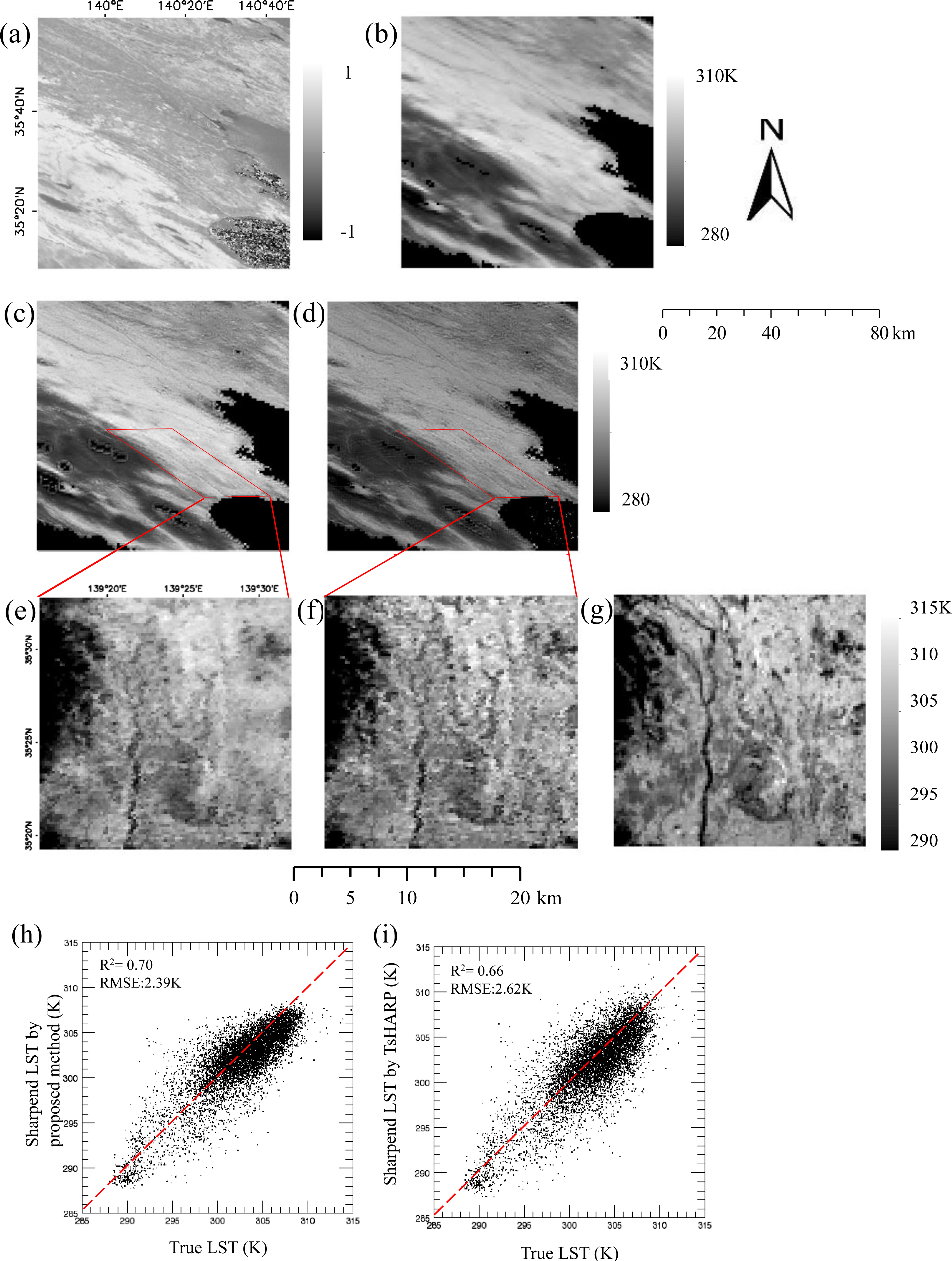
3.3. Application of MODIS Data
4. Discussion
5. Conclusions
Acknowledgments
Author Contributions
Conflicts of Interest
References
- Gillespie, A.; Rokugawa, S.; Matsunaga, T.; Cothern, J.S.; Hook, S.; Khale, A.B. Temperature and emissivity separation algorithm for advanced spaceborne thermal emission and reflection radiometer (ASTER) images. IEEE Trans. Geosci. Remote Sens 1998, 36, 1113–1126. [Google Scholar]
- Kato, S.; Yamaguchi, Y. Analysis of urban heat-island effect using ASTER and ETM+ Data: Separation of anthropogenic heat discharge and natural heat radiation from sensible heat flux. Remote Sens. Environ 2005, 99, 44–54. [Google Scholar]
- Kustas, W.; Anderson, M. Advances in thermal infrared remote sensing for land surface modeling. Agric. For. Meteorol 2009, 149, 2071–2081. [Google Scholar]
- Weng, Q. Thermal infrared remote sensing for urban climate and environmental studies: Methods, applications, and trends. ISPRS J. Photogramm. Remote Sens 2009, 64, 335–344. [Google Scholar]
- Gao, F.; Kustas, W.P.; Anderson, M.C. A data mining approach for sharpening thermal satellite imagery over land. Remote Sens 2012, 4, 3287–3319. [Google Scholar]
- Cao, X.; Onishi, A.; Chen, J.; Imura, H. Quantifying the cool island intensity of urban parks using ASTER and IKONOS data. Landsc. Urban Plan 2010, 96, 224–231. [Google Scholar]
- Zhan, W.; Chen, Y.; Zhou, J.; Li, J.; Liu, W. Sharpening thermal imageries: A generalized theoretical framework from an assimilation perspective. IEEE Trans. Geosci. Remote Sens 2011, 49, 773–789. [Google Scholar]
- Chen, Y.; Zhan, W.; Quan, J.; Zhou, J.; Zhu, X.; Sun, H. Disaggregation of remotely sensed surface temperature: A generalized paradigm. IEEE Trans. Geosci. Remote Sens 2014, in press.. [Google Scholar]
- Kustas, W.P.; Norman, J.M.; Anderson, M.C.; French, A.N. Estimating subpixel surface temperatures and energy fluxes from the vegetation index-radiometric temperature relationship. Remote Sens. Environ 2003, 86, 429–440. [Google Scholar]
- Agam, N.; Kustas, W.P.; Anderson, M.C.; Li, F.; Neale, C.M.U. A vegetation index based technique for spatial sharpening of thermal imagery. Remote Sens. Environ 2007, 107, 545–558. [Google Scholar]
- Zhan, W.; Chen, Y.; Zhou, J.; Wang, J.; Liu, W.; Voogt, J.; Zhu, X.; Quan, J.; Li, J. Disaggregation of remotely sensed land surface temperature: Literature survey, taxonomy, issues, and caveats. Remote Sens. Environ 2013, 131, 119–139. [Google Scholar]
- Anderson, M.C.; Norman, J.M.; Mecikalski, J.R.; Torn, R.D.; Kustas, W.P.; Basara, J.B. A multiscale remote sensing model for disaggregating regional fluxes to micrometeorological scales. J. Hydrometeorol 2004, 5, 343–363. [Google Scholar]
- Agam, N.; Kustas, W.P.; Anderson, M.C.; Li, F.; Colaizzi, P.D. Utility of thermal sharpening over Texas high plains irrigated agricultural fields. J. Geophys. Res.: Atmos 2007, 112. [Google Scholar] [CrossRef]
- Chen, X.; Yamaguchi, Y.; Chen, J.; Shi, Y. Scale effect of vegetation-index-based spatial sharpening for thermal imagery: A simulation study by ASTER data. IEEE Geosci. Remote Sens. Lett 2012, 9, 549–553. [Google Scholar]
- Sandhlot, I.; Rasmussen, K.; Andersen, J. A simple interpretation of the surface temperature/vegetation index space for assessment of surface moisture status. Remote Sens. Environ 2002, 79, 213–224. [Google Scholar]
- Tang, R.; Li, Z.; Tang, B. An application of the Ts-VI triangle method with enhanced edges determination for evapotranspiration estimation from MODIS data in arid and semi-arid regions: Implementation and validation. Remote Sens. Environ 2010, 114, 540–551. [Google Scholar]
- Merlin, O.; Duchemin, B.; Hagolle, O.; Jacob, F.; Coudert, B.; Chehbouni, G.; Dedieu, G.; Garatuza, J.; Kerr, Y. Disaggregation of MODIS surface temperature over an agricultural area using a time series of Formosat-2 images. Remote Sens. Environ 2010, 114, 2500–2512. [Google Scholar] [Green Version]
- Dominguez, A.; Kleissl, J.; Luvall, J.C.; Rickman, D.L. High-resolution urban thermal sharpener (HUTS). Remote Sens. Environ 2011, 115, 1772–1780. [Google Scholar]
- Yang, G.; Pu, R.; Zhao, C.; Huang, W.; Wang, J. Estimation of subpixel land surface temperature using and endmember index based technique: A case examination on ASTER and MODIS temperature products over a heterogeneous area. Remote Sens. Environ 2011, 115, 1202–1219. [Google Scholar]
- Jing, L.H.; Cheng, Q.M. A technique based on non-linear transform and multivariate analysis to merge thermal infrared data and higher-resolution multispectral data. Int. J. Remote Sens 2010, 31, 6459–6471. [Google Scholar]
- Liu, D.; Zhu, X. An enhanced physical method for downscaling thermal infrared radiance. IEEE Geosci. Remote Sens. Lett 2012, 9, 690–694. [Google Scholar]
- Rogers, S.; Girolami, M. A First Course in Machine Learning; Chapman & Hall/CRC, Taylor and Francis: Boca Raton, FL, USA, 2011. [Google Scholar]
- Jiang, Y.; Weng, Q. Estimating LST using a vegetation-cover-based thermal sharpening technique. IEEE Geosci. Remote Sens. Lett 2013, 10, 1249–1252. [Google Scholar]
- Bindhu, V.M.; Narasimhan, B.; Sudheer, K.P. Development and verification of a non-linear disaggregation method (NL-DisTrad) to downscale MODIS land surface temperature to the spatial scale of Landsat thermal data to estimate evapotranspiration. Remote Sens. Environ 2013, 135, 118–129. [Google Scholar]
- Dubrule, O. Comparing splines and kriging. Comput. Geosci 1984, 10, 327–338. [Google Scholar]
- Wahba, G. Spline Models for Observational Data; SIAM: Philadelphia, PA, USA, 1990. [Google Scholar]
- Boer, E.P.J.; de Beurs, K.M.; Hartkamp, A.D. Kriging and thin plate splines for mapping climate variables. Int. J. Appl. Earth Obs. Geoinf 2001, 3, 146–154. [Google Scholar]
- Chen, C.; Li, Y. A robust method of thin plate spline and its application to DEM construction. Comput. Geosci 2012, 48, 9–16. [Google Scholar]
- Wikle, C.K.; Berliner, L.M. A Bayesian tutorial for data assimilation. Phys. D 2007, 230, 1–16. [Google Scholar]
- Liu, Y.; Hiyama, T.; Yamaguchi, Y. Scaling of land surface temperature using satellite data: A case examination on ASTER and MODIS products over a heterogeneous terrain area. Remote Sens. Environ 2006, 105, 115–128. [Google Scholar]
- Qin, Z.; Karnieli, A.; Berliner, P. A mono-window algorithm for retrieving land surface temperature from Landsat TM data and its application to the Israel-Egypt border region. Int. J. Remote Sens 2001, 22, 3719–3746. [Google Scholar]
- Essa, W.; van der Kwast, J.; Verbeiren, B.; Batelaan, O. Downscaling of thermal images over urban areas using the land surface temperature–impervious percentage relationship. Int. J. Appl. Earth Obs.Geoinf 2013, 23, 95–108. [Google Scholar]


| No. | Data Type | Acquisition Time | Location | Landscape (Dominant Percentage) | Size (Thermal Resolution) |
|---|---|---|---|---|---|
| a | ASTER | 16 July 2010 | Inner Mongolia, China (44.6N, 116.0E) | Grassland (90%) | 256 × 256 (90 m) |
| b | ASTER | 26 April 2002 | Haihe river basin, China (38.3N, 114.7E) | Cropland (70%) | 256 × 256 (90 m) |
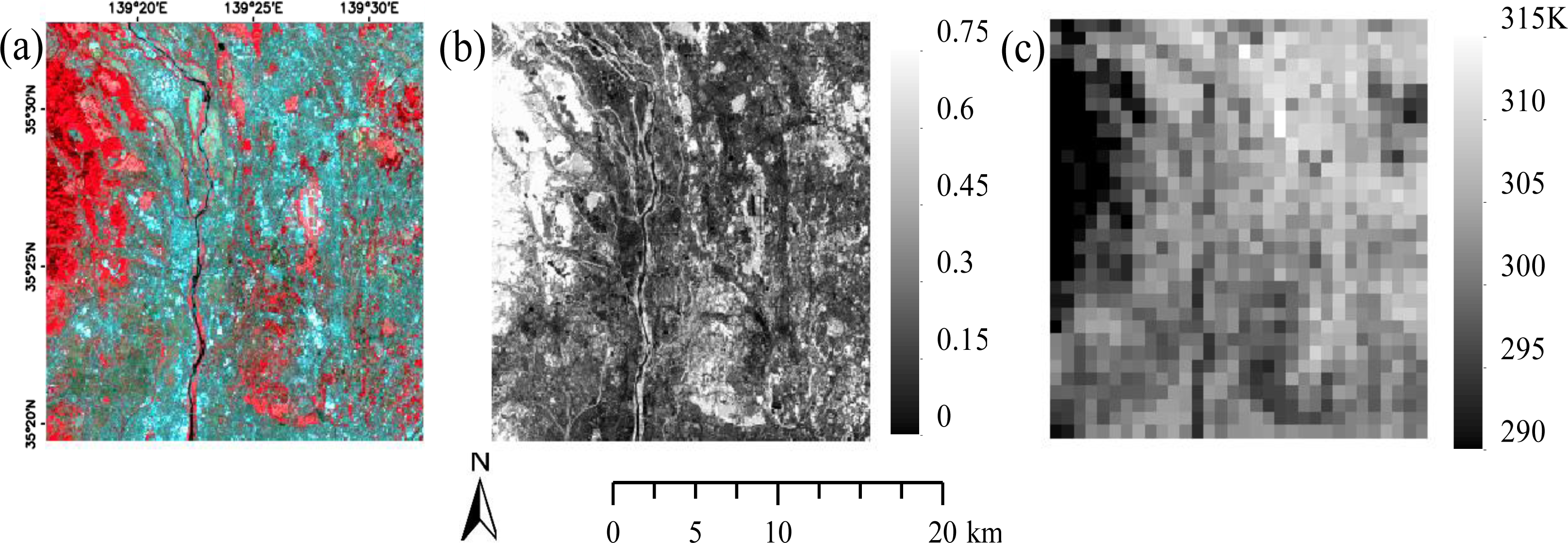
| c | ETM+ | 4 July 2001 | Aichi prefecture, Japan (35.2N, 136.8E) | Rural (70%) | 256 × 256 (60 m) |
| d | ASTER | 25 April 2004 | Yokohama city, Japan (35.4N, 139.4E) | Urban (60%) | 256 × 256 (90 m) |
© 2014 by the authors; licensee MDPI, Basel, Switzerland This article is an open access article distributed under the terms and conditions of the Creative Commons Attribution license (http://creativecommons.org/licenses/by/3.0/).
Share and Cite
Chen, X.; Li, W.; Chen, J.; Rao, Y.; Yamaguchi, Y. A Combination of TsHARP and Thin Plate Spline Interpolation for Spatial Sharpening of Thermal Imagery. Remote Sens. 2014, 6, 2845-2863. https://0-doi-org.brum.beds.ac.uk/10.3390/rs6042845
Chen X, Li W, Chen J, Rao Y, Yamaguchi Y. A Combination of TsHARP and Thin Plate Spline Interpolation for Spatial Sharpening of Thermal Imagery. Remote Sensing. 2014; 6(4):2845-2863. https://0-doi-org.brum.beds.ac.uk/10.3390/rs6042845
Chicago/Turabian StyleChen, Xuehong, Wentao Li, Jin Chen, Yuhan Rao, and Yasushi Yamaguchi. 2014. "A Combination of TsHARP and Thin Plate Spline Interpolation for Spatial Sharpening of Thermal Imagery" Remote Sensing 6, no. 4: 2845-2863. https://0-doi-org.brum.beds.ac.uk/10.3390/rs6042845