Article

Assessment of Coarse-Resolution Land Cover Products Using CASI Hyperspectral Data in an Arid Zone in Northwestern China

1
The Key Laboratory of Digital Earth Sciences, Institute of Remote Sensing and Digital Earth, Chinese Academy of Sciences, No.9 Dengzhuang South Road, Haidian District, Beijing 100094, China
2
Graduate University of Chinese Academy of Sciences, No.19A Yuquan Road, Haidian District, Beijing 100049, China
*
Author to whom correspondence should be addressed.
Remote Sens. 2014, 6(4), 2864-2883; https://0-doi-org.brum.beds.ac.uk/10.3390/rs6042864
Submission received: 12 December 2013 / Revised: 20 March 2014 / Accepted: 24 March 2014 / Published: 28 March 2014

Abstract

:
The accuracy of different coarse-resolution land cover products is an important consideration for product users at the regional or global scale, and different evaluation methods inevitably result in discrepancies in accuracy for the same land cover product. The remote sensing community has responded to this increased interest by improving methodologies for more accurately evaluating the correctness of land cover information. In this study, a pixel-based hierarchical classification strategy followed by an object-based classification method was applied to compact airborne spectrographic imager (CASI) hyperspectral data in order to produce highly accurate, high spatial resolution classification reference data. Some aspects of the fuzzy/conventional evaluation of MODIS land cover (MODISLC) (500 m) and GlobCover (300 m) data based on sub-pixel class fractions derived from high spatial resolution reference data at different thematic resolutions are also discussed. Relationships between homogeneity and fuzzy accuracy for two land cover products were obtained at different thematic resolutions. Additionally, the influences on the relationship resulting from the thematic resolution were also studied, and these are reported in this paper. Attempts were made to establish fuzzy/conventional evaluation rules for fuzzy classes, and the different performances of the fuzzy and conventional evaluations for hard/fuzzy labels were compared. The adjusted GlobCover accuracy after theoretical removal of the effect caused by spatial resolution was calculated based on the relationship between homogeneity and accuracy; the result was a higher accuracy than for MODISLC at the same thematic resolution. In addition, the different performance characteristics of the relationships between homogeneity and adjusted GlobCover accuracy/MODISLC accuracy at different thematic resolutions were compared and analyzed over the area where the CASI transects were obtained.

Graphical Abstract

1. Introduction

Global land cover maps provide thematic characterizations of the Earth’s surface, which are indispensable parameters required for the analysis of the state and dynamics of terrestrial ecosystems [1,2]. Land cover is an essential climate variable that describes the flow of carbon, water and energy through the biosphere [3], and its accuracy is of great importance for a wide range of scientific studies, such as studies of the carbon cycle, climate change, water balance and desertification or watershed degradation [47]. Recently, global land cover maps derived from satellite data have been widely used in biogeochemical and climate models, such as soil-vegetation-atmosphere transfer models (SVAT) and global circulation models (GCM) [8], to better understand biosphere-atmosphere interactions. Furthermore, changes in global land use and land cover have significant implications for ecosystem health, sustainable land management, nature conservation, food security and land-use planning [3,913].
Since global land cover datasets derived from AVHRR data became available in the 1990s, numerous additional global land cover datasets have been produced based on different remote sensing data sources and mapping initiatives, such as the International Geosphere-Biosphere Program (IGBP) DIScover dataset [14], the University of Maryland (UMD) land cover product [15], MODIS land cover (MODISLC) product [16], GLC2000 [17] and GlobCover [1820].
As global land cover products have been extensively applied in numerous studies, the accuracy of mapped land cover classes is an important concern for scientists using these products in regional or global studies. As a consequence, the assessment of the accuracy of land cover maps derived from satellite data has been an important preoccupation of the remote sensing community, and a variety of approaches, including direct [2129] and indirect [3034] methods, have been developed. Among them, the sub-pixel fractional error matrix has been an effective and accurate evaluation approach for coarse-resolution land cover products, since the sub-fractional error matrix was introduced as a more appropriate way for defining accuracy based on areal sampling units. Its advantage over a conventional error matrix is particularly evident in assessing areas containing mixed pixels, as often occurs in coarse-resolution maps [8]. The accuracy derived using a sub-pixel fraction error matrix is more representative of the confidence-based agreement between the classification map and reference data, since a pixel composed of several land cover classes cannot be 100% correct for a given class; however, the predicted class was considered to be either 100% correct or 100% incorrect using the conventional evaluation. Four land cover products (MODISLC, GLC2000, IGBP-DIScover and UMD) over Canada were evaluated using a sub-pixel fractional error matrix based on medium resolution (30 m) land cover data derived from Landsat TM/ETM+ imagery [8]. Ran et al. [26] also employed a sub-fractional error matrix to evaluate the four global land cover products (MODISLC, GLC2000, IGBP-DIScover and UMD) over China based on a 1:100,000 land cover map and analyzed the distribution of different error sources for each class.
In general, ambiguity in class labels leads to different interpretations. It is known that classification labels can be divided into two categories: “hard” classes and “soft/fuzzy” classes. The results of some previous studies have suggested that sub-pixel land cover mapping techniques based on continuous field characteristics may be preferable to “hard” classification approaches [8]. However, for “soft/fuzzy” classification, most applications retain the underlying assumption of crisp sets by constraining the sub-pixel proportions of the various classes to sum to unity. The assessment of the accuracy of these proportions of classes within pixels requires substantially different methods than for a thematic map in which each pixel is assigned to a single class [33]. Therefore, it is very important when evaluating the pixel-level accuracy of hard/fuzzy classification to achieve accurate information about the sub-pixel classes and their corresponding fractions within the coarse-resolution land cover pixel. It is evident that high-resolution remotely sensed data can provide the critical bridge needed for the evaluation of the accuracy of land cover products derived from coarse-resolution satellite imagery, such as MERIS (300 m) or MODIS (1 km) data.
In this paper, we show how a hyperspatial classification map derived from compact airborne spectrographic imager (CASI) hyperspectral imagery was employed as a reference for the evaluation of MODISLC with hard classes and GlobCover, which includes fuzzy classes, based on the obtained sub-pixel classes and fractions. The major objectives of this study were:
  • to evaluate the MODISLC product using conventional and fuzzy evaluation methods at different thematic scales;
  • to evaluate GlobCover using conventional and fuzzy evaluation at different thematic scales;
  • to compare the fuzzy and conventional evaluation results for fuzzy and hard classes;
  • to calculate the theoretical real difference between the accuracy of MODISLC and GlobCover at different thematic resolutions.

2. Materials

2.1. Study Site

The study was carried out in the Heihe River Basin, China’s second largest inland river basin. The study area is located between 97°24′ and 102°10′E and 37°41′ and 42°42′N and covers an area of approximately 130,000 km2. The landscape within the basin is diverse, comprising upstream and downstream elements, including glacier, frozen soil, alpine meadow, forest, irrigated crops, riparian ecosystems, desert and Gobi (Figure 1) [35]. The middle reaches of the Heihe River are dominated by a temperate arid climate with an annual precipitation of 140 mm, an annual evapotranspiration of 1400–2800 mm, an annual sunshine amount of 3000–4000 hours and an average annual temperature of 6 °C–8 °C. The altitude range is 1000–2000 m. The representative scenery consists of a staggered landscape of plain oasis and Gobi desert comprising sparse native vegetation and numerous areas of artificial vegetation. Thus, it is very difficult to accurately evaluate the accuracy of a land cover product derived from coarse-resolution remote sensing data (such as the 300-m GlobCover or 500-m MODISLC product) in such a heterogeneous region. Furthermore, as this area is an irrigated district managed by farmers and the local government, the overall land cover patterns, including cropland, built-up areas and barren land, shelter forest and sparse shrubs, are very stable. Therefore, it can be assumed that the main land cover patterns did not change during the 3-year period of 2009–2012.

2.2. CASI Transects

In this study, compact airborne spectrographic imager (CASI-1500) imagery acquired on 29 June 2012, provided by Heihe Watershed Allied Telemetry Experimental Research (HiWATER) and launched by the National Natural Science Foundation of China (NSFC) [35], was used to evaluate MODISLC and GlobCover. Details of the CASI imagery are shown in Table 1. The imaging region for the CASI airborne sensor consisted of two long transects (Figure 1) covering 85.6 km × 1.4 km and 70 km × 1.4 km over Gaotai and Linze counties in the middle reaches of the Heihe river basin. The CASI transects covered Gobi, various irrigated crops, grassland and the river. Furthermore, due to the CASI imagery used in this study being acquired at the peak of the vegetation growth season when the different vegetation types provided obvious differences in spectral features, it is reliable for obtaining accurate land cover classification based on CASI hyperspectral data.

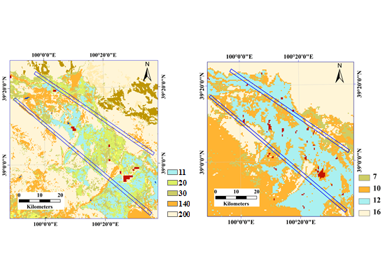
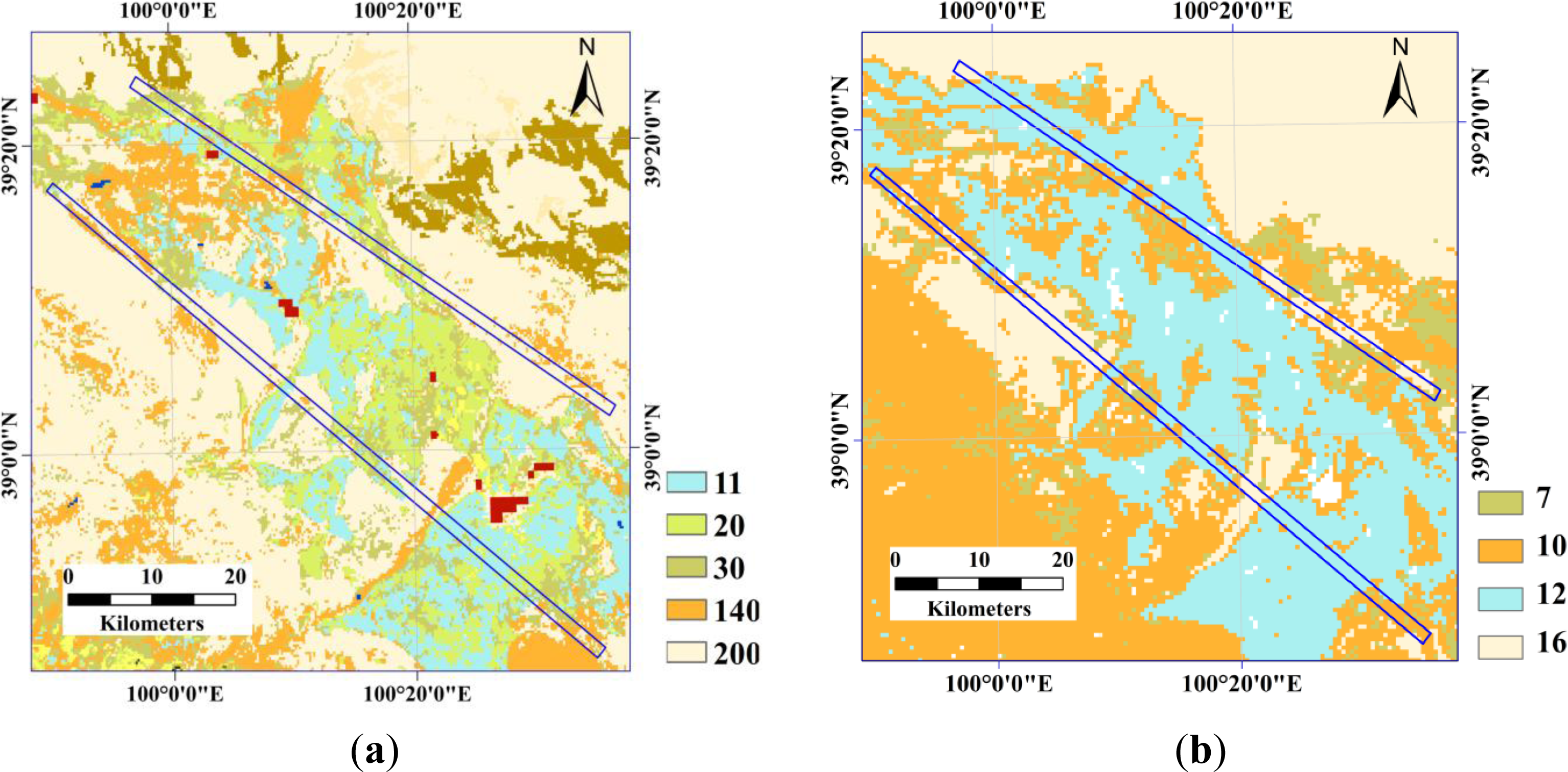
2.3. Coarse-Resolution Land Cover

Current satellite missions (SPOT, MODIS and MERIS) have become an increasingly vital component of the global observing system used for the monitoring of land cover and its dynamics [31]. In this paper, two commonly used coarse-resolution satellite land cover products are evaluated over the area where the CASI transects were obtained. A basic description of the two products is given in Table 2.
GlobCover is a European Space Agency (ESA) initiative, which began in 2005 in partnership with the Joint Research Center (JRC), the European Environmental Agency (EEA), the Food and Agriculture Organization (FAO), the United Nations Environment Program (UNEP), the Global Observation of Forest Cover and Land Dynamics (GOFC-GOLD) and the International Geosphere-Biosphere Program (IGBP). The available GlobCover land cover products include two versions: GlobCover, released in late September 2008, and GlobCover 2009, released on 1 December 2010 [1820]. The recently released GlobCover 2009 for the year 2009 was used in this paper in order to match the acquisition time of the CASI aerial imagery. The MODISLC product, developed by Boston University in cooperation with the MODIS Land Team from the National Aeronautics and Space Administration (NASA), provides data characterizing five global land cover classification systems [16]. The first version was made available in 2001, and it has been updated yearly since then. The first land cover classification scheme identifying 17 land cover classes defined by the IGBP from MCD12Q1 V051 [1] for the year 2012 was used in this study.

2.4. Ground Survey Data

Prior knowledge about land cover types is very important for accurately classifying remote sensing images using an automatic classification algorithm. Even though some land cover types in high spatial resolution (1 m) imagery can be identified by visual interpretation, a ground survey to obtain land cover information was carried out during July 2012, and this was very helpful for providing accurate prior knowledge about the different land cover types in the CASI hyperspectral imagery (Figure 1). A total of 139 accessible ground survey sites were surveyed within CASI transects, and the GPS locations of the individual survey sites can be seen in Figure 1. These data, together with manual interpretation of the CASI images, were used to select high-quality sample pixels for the different land cover types. We then generated random training and testing data in the proportion of 6:4 within the sample dataset.

3. Methodology

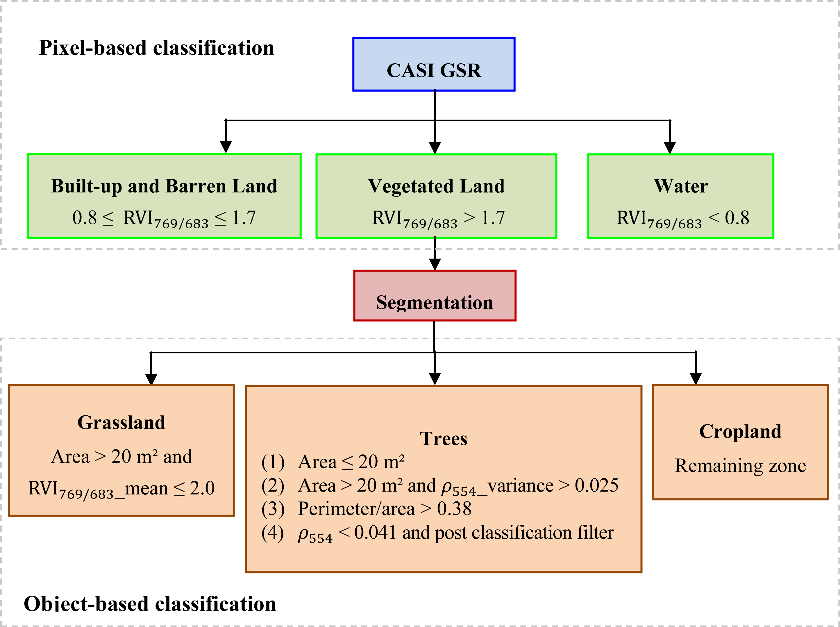
3.1. Classification of CASI Transects

In this study, a high spatial resolution classification based on CASI imagery was used as the reference data for evaluating the accuracy of the coarse-resolution satellite-based land cover products. The aerial classification database consisted of a 1-m resolution land cover database classified into five land cover types based on the ground survey data, visual interpretation of the CASI imagery and the requirement that classes match the labels used for the GlobCover and MODISLC sub-pixel classes. The five land cover types included trees, grassland, water, cropland and built-up and barren land. For the hyperspatial aerial classification dataset, the preparatory and classification steps included the following.
  • The CASI DN values were first radiometrically corrected using calibration coefficients provided by laboratory calibration (gains and offsets). Then, atmospheric correction was carried out using the MOTRAN 4 model, which is embedded in the ENVI/FLAASH module [36], in order to derive the ground surface reflectance (GSR). The input parameters were set based on the location, sensor type and ground weather conditions observed on the day the image was acquired. Then, the CASI GSR was geometrically registered using the CASI pre-processing software (ProcManager) with required flight parameters and airborne POS data. During this registration process, each pixel was resampled to 1-m resolution and the UTM projection (WGS 84) using the nearest-neighbor method.
  • A simple pixel-level ratio vegetation index (RVI) based on ρ769 (NIR) and ρ683 (red) reflectance bands was used to accurately separate the vegetated, built-up and barren land and water pixels.
  • The vegetated land area was segmented into individual objects using a blob coloring algorithm based on spatial neighborhoods. For example, spatially adjacent vegetated pixels were merged into one object; if there were no other vegetated pixels adjacent to a pixel, it was defined as an object.
  • Relatively small vegetated objects of a single type (shrubs) were characterized by a specific small area threshold (Figure 2).
  • Relatively large vegetated objects of a single type included grassland and spatially continuous trees. The grassland class was typically characterized by relatively large areas and low RVI thresholds. Continuous trees with different growth status were discriminated based on the large areas they covered and also the variance threshold (Figure 2) for the reflectance of the green band (ρ554). A shape index (Figure 2) giving the ratio of the perimeter to the area of an object was used to extract tree-covered areas with a specific geometric shape, such as green belts along roads.
  • Relatively large vegetated objects of mixed types consisted of cropland and shelterbelt mixed with cropland. The reflectance threshold (Figure 2) of the green band (ρ554) was applied to extract a portion of shelterbelt; however, defining the remaining pixels (excluding the extracted shelterbelt) as cropland would have misclassified some trees in the shelterbelts as cropland, which is erroneous. To address this problem, we developed a post-classification process for mixed vegetation that used a moving 3 × 3 window to filter the resulting classification. If the center pixel of the window was cropland and at least one ‘tree’ pixel was present in the window, the center pixel was moved to the tree class.
As shown in Figure 2, a hierarchical classification scheme [3740] was employed to classify the CASI hyperspectral imagery: different hierarchical levels were separated using a pixel-based classification based on reflectance spectra, and different vegetation types were discriminated using object-based classification based on geometric and spectral features of objects segmented according to the spatial adjacent relationship. In the pixel-based classification, RVI thresholds discriminating three land cover types were set when the classification accuracy of the testing sample pixels from three land cover types reached its maximum value; in the object-based classification, thresholds discriminating a specific land cover type were set when the accuracy of the testing sample pixels from the specific land cover reached its maximum value. The land cover types in the CASI transects were mapped according to the above hierarchical classification process, as illustrated in Figure 3. (The result for one sub-region within the CASI transects is shown).

3.2. Evaluation of Coarse-Resolution Land Cover over the Area of the Continuous CASI Transects

GlobCover and MODISLC land cover were reprojected on to a UTM projection using the same projection parameters as the CASI data (UTM N47, WGS-84). The boundary coordinates of each GlobCover (300 m) or MODISLC (500 m) pixel could be calculated using the central UTM coordinates of the pixel. The pixels that were completely covered by the CASI transects according to a comparison of the coordinate ranges in the CASI transects and coarse-resolution pixels were then selected for evaluation in the next step. The number of pixels selected from GlobCover and MODISLC are shown in Table 3.
As shown in Table 3, five GlobCover land cover classes (Classes 11, 20, 30, 140, 200) and four MODISLC land cover classes (Classes 12, 7, 10, 16) were present within the area of the CASI transects; their corresponding spatial distributions are shown in Figure 4. In this study, the following steps were performed for each coarse-resolution land cover pixel: (1) the location of the center of the coarse-resolution pixel was determined; (2) the pixel’s footprint was located in the CASI transects; (3) the proportions of the different land cover types within the footprint were calculated according to the hyperspatial classification; (4) the dominant fraction and corresponding dominant class within the footprint was determined.
In the evaluation process using high spatial resolution reference data, open shrubland (Class 7) in MODISLC was considered to agree with the trees ‘class’ in the reference data, as the trees in the study area consist of a large number of young trees and groves, whose heights and crowns are very close to those of shrubs in the desert. Class 200 in GlobCover and Class 16 in MODISLC were considered to agree with ‘built-up and barren land’ in the reference data. As built-up areas account for only a tiny proportion of the enlarged coarse-resolution land cover pixels, this was unlikely to have much impact on these evaluation results.
In MODISLC, each class definition describes a “hard” label that represents only one type of class. The conventional and fuzzy methods used in this study for the evaluation of MODISLC “hard” classes can be summarized as follows.
  • Fuzzy: The accuracy of the pixel is equal to the percentage of hyperspatial reference pixels that agree with the class of the coarse-resolution pixel based on the sub-fraction error matrix [8].
  • Conventional: The accuracy of the pixel is a Boolean value. The coarse-resolution pixel is considered to be 100% correct when it agrees with the dominant class or 0% correct when it disagrees.
For GlobCover, the evaluation methods for MODISLC described above are also suitable for other hard classes in GlobCover. However, some classes describe “fuzzy” labels that consist of a variety of sub-pixel classes and their corresponding proportions (e.g., Class 20 consists of mosaic cropland (50%–70%) and vegetation (grassland/shrubland/forest) (20%–50%)). The sub-pixel class fraction derived for each coarse-resolution pixel offers an additional option for assessing fuzzy classification: a set of rules can be established to define the relationship between reference and classification data [8]. Strict conventional and fuzzy evaluation rules were established in this study for “fuzzy” GlobCover classes based on a comprehensive consideration of the correctness of the classes involved in the definition of each label. The process is shown below, taking Class 20 as an example.
  • Fuzzy: The accuracy is determined according to the different pre-conditions, as shown in Table 4.
  • Conventional: The coarse-resolution pixel is considered to be 100% correct when cropland agrees with the reference-based dominant class and the percentage of natural vegetation is not less than 20%; otherwise, the pixel is considered to be 0% correct.
Both conventional and fuzzy evaluation methods were performed for MODISLC and GlobCover over the area covered by the continuous CASI transects. The evaluations of the two methods for each coarse-resolution land cover type were compared and the difference in accuracy achieved using the fuzzy and conventional evaluation methods for hard classes, and fuzzy classes were also analyzed. In addition, the accuracy of MODISLC and GlobCover were also evaluated for the different thematic resolutions shown in Table 3, and the relationships between homogeneity and classification accuracy were explored. All analyses performed in this study were based on conventional and fuzzy accuracies generated using coarse-resolution land cover and hyperspatial resolution reference land cover data.

4. Results and Discussion

4.1. Accuracy of CASI Hyperspatial Classification

The classification accuracy of the CASI transects was assessed using the test data and was found to have an overall accuracy of 95.07% and a kappa coefficient of 0.93, as shown in Table 5. This shows that the CASI land cover map could provide reliable reference data for validation of the GlobCover product.

4.2. Influence of Homogeneity on Accuracy of MODISLC and GlobCover

The homogeneity of each coarse-resolution pixel can be measured using the proportion of the dominant land cover type in the hyperspatial reference data: the greater the dominant fraction, the more homogeneous the coarse-resolution pixel will be. In this study, the homogeneity over the area covered by the continuous CASI transects was classified into six cluster members based on the dominant fraction of each coarse-resolution pixel (40%–50%, 50%–60%, 60%–70%, 70%–80%, 80%–90%, 90%–100%). The relationships between the homogeneity and corresponding classification accuracy of cluster members for MODISLC and GlobCover at different thematic resolutions are presented in Figure 5. The x-coordinate of a point on this graph is the average dominant fraction, which represents the average homogeneity over a given cluster, while the y-coordinate gives the corresponding average accuracy achieved by either fuzzy or conventional evaluation. For fuzzy evaluation, the 1:1 line defines the maximum achievable accuracy for a given homogeneity, while the difference in y-coordinates between a point and the 1:1 line represents the error of the classification method [8].
Both conventional and fuzzy evaluation were applied to MODISLC and GlobCover using the original thematic classes. It can be seen in Figure 5 that the conventional accuracy of a cluster (70%–80%) in MODISLC is higher than the maximum achievable accuracy for a given homogeneity that results from considering that the pixel is 100% correct in the conventional evaluation. This means that the accuracy of the pixel is overestimated, which to some extent indicates that the fuzzy evaluation method is more reasonable. It can be seen from Figure 5 that the conventional accuracy is higher than the fuzzy accuracy for MODISLC with hard labeling, whereas the opposite—conventional accuracy lower than the fuzzy accuracy—is true for GlobCover with fuzzy labeling. The reason for this phenomenon will be discussed in the next section. The graph also indicates that the relationship between the fuzzy accuracy and homogeneity is more significant than the conventional accuracy and that the difference between the fuzzy accuracy and the conventional accuracy narrows with increasing pixel homogeneity.
In Figure 5, there is a general increasing trend in classification accuracy with increasing pixel homogeneity as a result of the relative unambiguity of pure pixel labeling. However, in the case of MODISLC, there is an obvious decrease in accuracy in highly homogeneous areas with a dominant fraction of 90%–100%. These pixels with high homogeneity are classified as grassland or shrubland and account for a tiny proportion of the reference data. For GlobCover, in contrast, the accuracy continuously increases with increasing homogeneity, which indicates that GlobCover agrees better with the reference data than MODISLC when the labeling is unambiguous. Further analysis of the spatial distribution of the disagreement between GlobCover and the reference data reveals that the largest differences between them are found in transition zones between desert and oasis cropland.
A smaller number of thematic classes will produce a higher dominant fraction and more homogeneous land cover, and vice versa [8]. In this study, fuzzy evaluation was performed for two coarse-resolution land cover types at different thematic resolutions. It can be seen from Figure 5 that the accuracy at lower thematic resolution is higher than that at higher thematic resolution for MODISLC with hard labels, because the lower thematic resolution reduces the number of labeling errors caused by mislabeling, whereas the accuracy with the original thematic classes is a little bit higher than that obtained using three thematic classes for GlobCover. This is caused by the influence of the evaluation on the fuzzy labeling. For GlobCover, the coefficients of determination (R2) for the regression relationship between homogeneity and accuracy exhibit an increasing trend as the number of thematic classes decreases; in contrast, there is a decreasing trend in the case of MODISLC as a result of the mislabeling that occurs in highly homogeneous regions (see Figure 5).

4.3. Comparison of Fuzzy and Hard Class Accuracies

In order to better understand the different performances of the fuzzy and hard class labeling, we selected all GlobCover Class 20 pixels in the region of the CASI transects for accuracy evaluation. In this case, the fuzzy and conventional accuracies of each Class 20 pixel were calculated based on the evaluation rules established for the fuzzy class (Table 4). In addition, “cropland”, which is the dominant class in the Class 20 definition, was used as the hard label for all the pixels. It can be clearly seen from Figure 6 that the maximum achievable fuzzy accuracy of the hard class is the dominant class fraction of a coarse-resolution pixel, whereas the fuzzy accuracy for the fuzzy class might be higher than the dominant class fraction of a coarse-resolution pixel. To find the maximum achievable accuracy of the fuzzy class, it is necessary to carry out further analysis based on different preconditions, as listed in Table 4.
The conventional accuracy for the fuzzy class is very low and is characterized by a decreasing trend with increasing homogeneity as a result of the evaluation rule, which is stricter than the conventional evaluation for the hard class and which focuses on the correctness of both the dominant class and sub-dominant classes. It, therefore, becomes harder for a coarse-resolution pixel to be considered 100% correct, especially in a highly homogeneous area, where there are fewer sub-dominant classes. For the hard class, the conventional accuracy is higher than the dominant fraction and increases with increasing homogeneity.
Figure 6 shows that the fuzzy accuracy for the fuzzy class is higher than that for the hard class. It can also be seen that the difference between the accuracies is very small and becomes narrower with increasing homogeneity. In contrast, the difference between the conventional accuracy for the fuzzy class and that for the hard class is large and becomes wider with increasing homogeneity. From another perspective, it can also be seen that the variation in the fuzzy accuracy for the hard and fuzzy classes is small, whereas the variation in the conventional accuracy for the hard and fuzzy classes is relatively large. The fuzzy evaluation method, therefore, has a more stable performance.
However, the variation characteristic of the fuzzy accuracy for the fuzz class, as shown in Figure 6, is particular to the coarse-resolution pixels, where the dominant class of the fuzz label agrees with the reference-based dominant class, and sub-dominant classes also exist in the reference data. Within the CASI transects, the reference-based dominant class of a majority of pixels labeled with Class 20 is cropland, and natural vegetation also exists in the pixels, which indicates that Class 20 in GlobCover performs in good agreement with the reference data over the study area.

4.4. Comparison of MODISLC and GlobCover Accuracy

As fuzzy accuracy is a more reasonable representative of the “true” accuracy of coarse-resolution land cover and is more significantly related to the homogeneity, all of the performance analysis described in this section was based on the fuzzy accuracy. The average homogeneities and average accuracies of MODISLC and GlobCover over the CASI transects at different thematic resolutions are listed in Table 6. It can be seen that the average homogeneity shows an increasing trend with decreasing spatial and thematic resolution and also that the average accuracy for MODISLC and GlobCover with hard thematic labels (green cells in Table 6) shows an increasing trend with increasing average homogeneity. This supports the conclusion of a previous study [8] that spatial resolution and thematic resolution both affect pixel homogeneity, which, in turn, determines the evaluated accuracy for the coarse-resolution pixel. However, it should be noted that average accuracies for GlobCover, including fuzzy thematic labels (yellow cells in Table 6), present higher accuracy than the corresponding accuracies for GlobCover with three thematic hard classes, which could be explained by the fact that fuzz accuracy for fuzz class is higher than that for hard class, as illustrated in Figure 6.
Differences in spatial resolution, the projection system and the sensor point spread function represent one of the main difficulties in comparing the different coarse-resolution land cover datasets [30]. In general, in previous land cover comparison studies [3033], land cover datasets were spatially resampled and translated into a common legend that accommodated all the land cover categories on an aggregated level, so that the comparison can be performed. However, the accuracy of one coarse-resolution map at different spatial resolutions could be simulated based on a theoretical relationship between the image spatial resolution and the accuracy achieved by combining the resolution, homogeneity and accuracy relationships [8]. In this study, we used this approach to realize the accuracy comparison between land cover maps with different spatial resolutions without resampling for land cover. The quantitative mathematical relationships (Figure 5b) achieved between homogeneity and fuzzy accuracy for GlobCover at different thematic resolutions were used to calculate the adjusted GlobCover accuracy by taking the homogeneity at the MODISLC spatial resolution as the input x-value. The adjusted GlobCover accuracy represents the accuracy of GlobCover labeling at the spatial resolution of MODISLC; theoretically, it eliminates the influence of the spatial resolution on the accuracy. The difference between the accuracy and adjusted accuracy for GlobCover represents the influence of the error due to the spatial resolution, as illustrated in Table 6.
It can be seen from Table 6 that the average adjusted GlobCover accuracy is higher than the MODISLC accuracy at the same thematic resolution (three classes and two classes), which indicates that the GlobCover classification method is theoretically more accurate than MODISLC’s over the area of the CASI transects after the removal of the of the effects due to the spatial and thematic resolution.
In this analysis, different performances of the adjusted GlobCover accuracy and MODISLC accuracy in areas with different homogeneities at different thematic resolution scales were compared. The different types of difference shown in Table 7 are explained below the table. From the values of difference1 and difference2 shown in Table 7, it can be seen that a lower thematic resolution can produce almost the same increasing effect on the adjusted GlobCover accuracy in areas with different degrees of homogeneity, whereas a lower thematic resolution could more clearly affect the MODISLC accuracy in heterogeneous areas than in homogeneous areas. Furthermore, a comparison between the magnitude of difference3 and difference4 shows that a lower thematic resolution can reduce the gap between the MODISLC and GlobCover accuracies. Difference4 is higher than difference3 for areas with a 90%–100% dominant fraction as a result of the MODISLC mislabeling in homogeneous areas that were analyzed in the previous section.

5. Conclusions

In this study, fine-scale remotely sensed data from an area of continuous CASI transects provided a good opportunity to obtain sub-pixel class fractions and to determine the dominant class type in coarse-resolution land cover pixels. This is crucial for assessing the accuracy of coarse-resolution land cover products. A highly accurate hyperspatial aerial classification map was produced and used as the reference data for conventional and fuzzy evaluation of MODISLC and GlobCover land cover products. For fuzzy classes in GlobCover, we attempted to establish suitable evaluation rules. Factors influencing the accuracy included the homogeneity, spatial resolution and thematic resolution, and these were all fully considered in the comparative analysis. The results of the analysis showed that the relationship between fuzzy accuracy and homogeneity is more significant than conventional accuracy, and that the difference between the fuzzy accuracy and the conventional accuracy gets narrower with increasing pixel homogeneity. GlobCover was in better agreement with the reference data than MODISLC when the labeling was unambiguous. The variation in the fuzzy accuracy for both hard and fuzzy classes was small, whereas the variation in the conventional accuracy for hard and fuzzy classes was relatively large. Hence, the fuzzy evaluation was more stable under different types of labeling, and in theory, the GlobCover classification product provided a higher mapping accuracy than MODISLC after removal of the effects due to the spatial and thematic resolution over the area of the CASI transects.
However, the conclusions based on the above analysis are particular to the study area used and, more specifically, to the datasets and methods used to derive the relationships concerning accuracy, homogeneity, spatial resolution and thematic resolution. In addition, other factors also introduced unavoidable errors into the accuracy evaluation. These included misregistration between the coarse-resolution land cover and hyperspatial reference data and errors in the regression relations between homogeneity and accuracy at different thematic resolutions. The heterogeneity derived from the reference data showed that the grassland and open shrub over the study area can be described by a mosaic label, such as GlobCover Class 20, or can be mapped using higher spatial resolution satellite imagery, which could improve the mapping accuracy for grass and shrub in heterogeneous zones.
The assertions contained in this study must be qualified by stating that they apply to the performance of datasets over a small-scale region; further studies should focus on a larger area. However, aerial remote sensing datasets are costly and of limited availability, and so, this poses significant challenges in evaluating land cover products at continental or global scales. High resolution and multispectral satellite data covering larger areas, such as WorldView, GeoEye and QuickBird data, could be considered as alternatives.

Acknowledgments

The authors gratefully acknowledge the financial support provided for this research by the National Natural Science Foundation of China (91125003, 41222008) and the help of all the contributors to the Heihe Watershed Allied Telemetry Experimental Research (HiWATER).

Author Contributions

Zhihui Wang and Liangyun Liu conceived and designed the research. Zhihui Wang led the development of the CASI classification algorithms, assessment of coarse-resolution land cover products and manuscript writing. Liangyun Liu assisted with developing the research design, interpreted results and assisted with manuscript revision. All authors contributed with ideas, writing and discussions.

Conflicts of Interest

The authors declare no conflict of interest.

Reference

  1. Filed, M.A.; Sulla-Menashe, D.; Tan, B.; Schneider, A.; Ramankutty, N.; Sibley, A.; Huang, X. MODIS collection 5 global land cover: Algorithm refinements and characterization of new datasets. Remote Sens. Environ 2010, 114, 168–182. [Google Scholar]
  2. Hüttich, C.; Herold, M.; Wegmann, M.; Cord, A.; Strohbach, B.; Schmullius, C.; Dech, S. Assessing effects of temporal compositing and varying observation periods for large-area land-cover mapping in semi-arid ecosystems: Implications for global monitoring. Remote Sens. Environ 2011, 115, 2445–2459. [Google Scholar]
  3. Herold, M.; Mayaux, P.; Woodcock, C.E.; Baccini, A.; Schmullius, C. Some challenges in global land cover mapping: An assessment of agreement and accuracy between existing 1 km datasets. Remote Sens. Environ 2008, 112, 2538–2556. [Google Scholar]
  4. Bonan, G.B.; Oleson, K.W.; Vertenstein, M.; Levis, S.; Zeng, X.B.; Dai, Y.J. The land surface climatology of the community land model coupled to the NCAR community climate model. J. Clim 2002, 15, 3123–3149. [Google Scholar]
  5. Zhang, K.; Kimball, J.S.; Mu, Q.; Jones, L.A.; Goetz, S.J.; Running, S.W. Satellite based analysis of northern ET trends and associated changes in the regional water balance from 1983 to 2005. J. Hydrol 2009, 379, 92–110. [Google Scholar]
  6. Lambin, E.F.; Geist, H.J.; Lepers, E. Dynamics of land-use and land cover change in tropical regions. Annu. Rev. Environ. Resour 2003, 28, 205–241. [Google Scholar]
  7. Feddema, J.J.; Oleson, K.W.; Bonan, G.B.; Mearns, L.O.; Buja, L.E.; Meehl, G.A.; Washington, W.M. The importance of land-cover change in simulating future climates. Science 2005, 310, 1614–1678. [Google Scholar]
  8. Latifovic, R.; Olthof, I. Accuracy assessment using sub-pixel fractional error matrices of global land cover products derived from satellite data. Remote Sens. Environ 2004, 90, 153–165. [Google Scholar]
  9. Wu, W.; Pauw, E.D.; Zucca, C. Using remote sensing to assess impacts of land management policies in the Ordos Rangelands in China. Int. J. Digit. Earth 2013, 6, 81–102. [Google Scholar]
  10. García-Mora, T.J.; Mas, J.F.; Hinkley, E.A. Land cover mapping applications with MODIS: A literature review. Int. J. Digit. Earth 2012, 5, 63–87. [Google Scholar]
  11. Foley, J.A.; DeFries, R.; Asner, G.P.; Barford, C.; Bonan, G.; Carpenter, S.R.; Coe, M.T.; Daily, G.C.; Gibbs, H.K.; Helkowski, J.H.; et al. Global consequences of land use. Science 2005, 309, 570–574. [Google Scholar]
  12. Sutherland, W.J.; Adams, W.M.; Aronson, R.B.; Aveling, R.; Blackburn, T.M.; Blackburn, S; Broad, G.; Cote, I.M.; Cowling, R.M.; da Fonseca, G.A.B.; et al. One hundred questions of importance to the conservation of importance to the conservation of global biological diversity. Conserv. Biol 2009, 23, 557–567. [Google Scholar]
  13. Dougill, A.; Trodd, N. Monitoring and modelling open savannas using multisource information: Analysis of Kalahari studies. Glob. Ecol. Biogeogr 1999, 8, 211–221. [Google Scholar]
  14. Loveland, T.R.; Reed, B.C.; Brown, J.F.; Ohlen, D.O.; Zhu, Z.; Yang, L.; Merchant, J.W. Development of a global land cover characteristics database and IGBP DISCover from 1 km AVHRR data. Int. J. Remote Sens 2000, 21, 1303–1330. [Google Scholar]
  15. Hansen, M.C.; Defries, R.S.; Townshend, J.; Sohlberg, R. Global land cover classification at 1 km spatial resolution using a classification tree approach. Int. J. Remote Sens 2000, 21, 1331–1364. [Google Scholar]
  16. Friedl, M.A.; McIver, D.K.; Hodges, J.C.F.; Zhang, X.Y.; Muchoney, D.; Strahler, A.H.; Woodcock, C.E.; Gopal, S.; Schneider, A.; Cooper, A.; et al. Global land cover mapping from MODIS: Algorithms and early results. Remote Sens. Environ 2002, 83, 287–302. [Google Scholar]
  17. Bartholomé, E.; Belward, A.S. GLC2000: A new approach to global land cover mapping from Earth observation data. Int. J. Remote Sens 2005, 26, 1959–1977. [Google Scholar]
  18. Bicheron, P.; Defourny, P.; Brockmann, C.; Schouten, L.; Vancutsem, C.; Huc, M.; Bontemps, S.; Leroy, M.; Achard, F.; Herold, M.; et al. GLOBCOVER: Products Description and Validation Report 2008. Available online: http://due.esrin.esa.int/GlobCover/ (accessed on 18 Sepetember 2013).
  19. Arino, O.; Bicheron, P.; Achard, F.; Latham, J.; Witt, R.; Weber, J.L. GlobCover: The most detailed portrait of the Earth. ESA Bull.-Eur. Space Agency 2008, 136, 24–31. [Google Scholar]
  20. Bontemps, S.; Defourny, P.; Bogaert, E.V.; Arino, O.; Kalogirou, V.; Perez, J.R. GLOBCOVER 2009: Products Description and Validation Report 2011. Available online: http://due.esrin.esa.int/GlobCover/ (accessed on 18 Sepetember 2013).
  21. Cihlar, J.; Latifovic, R.; Beaubien, J.; Guindon, B.; Palmer, M. TM-based accuracy assessment of a land cover produce for Canada derived from SPOT VEGETATION data. Can. J. Remote Sens 2003, 29, 154–170. [Google Scholar]
  22. Muchoney, D.M.; Strahler, A.H. Pixel- and site-based calibration and validation methods for evaluating supervised classification of remotely sensed data. Remote Sens. Environ 2002, 81, 290–299. [Google Scholar]
  23. Sedano, F.; Gong, P.; Ferrão, M. Land cover assessment with MODIS imagery in southern African Miombo ecosystems. Remote Sens. Environ 2005, 98, 429–441. [Google Scholar]
  24. Stehman, S.; Wickham, J.D.; Wade, T.G.; Smith, J. Designing a multi-objective multi-support accuracy assessment of the 2001 National Land Cover Data (NLCD 2001) of the conterminous United States. Photogramm. Eng. Remote Sens 2008, 74, 1561–1571. [Google Scholar]
  25. Liang, S.L.; Fang, H.L.; Chen, M.Z.; Shuey, C.J.; Walthall, C.; Daughtry, C.; Morisette, J.; Schaaf, C.; Strahler, A. Validating MODIS land surface reflectance and albedo products: Methods and preliminary results. Remote Sens. Environ 2002, 83, 149–162. [Google Scholar]
  26. Ran, Y.; Li, X.; Lu, L. Evaluation of four remote sensing based land cover products over China. Int. J. Remote Sens 2010, 31, 391–401. [Google Scholar]
  27. Elatawneh, A.; Kalaitzidis, C.; Petropoulos, G.P.; Schneider, T. Evaluation of diverse classification approaches for land use/cover mapping in a Mediterranean region utilizing Hyperion data. Int. J. Digit. Earth 2014, 7, 194–216. [Google Scholar]
  28. An, Y.; Zhao, W.; Zhang, Y. Accuracy assessments of the GLOBCOVER dataset using global statistical inventories and FLUXNET site data. Acta Ecol. Sin 2012, 32, 314–320. [Google Scholar]
  29. Fernandes, R.; Fraser, R.; Latifovic, R.; Cihlar, J.; Beaubien, J.; Du, Y. Approaches to fractional land cover and continuous field mapping: A comparative assessment over the BOREAS study region. Remote Sens. Environ 2004, 89, 234–251. [Google Scholar]
  30. Pérez-Hoyos, A.; García-Haro, F.J.; San-Miguel-Ayanz, J. Conventional and fuzzy comparisons of large scale land cover products: Application to CORINE, GLC2000, MODIS and GlobCover in Europe. ISPRS J. Photogramm. Remote Sens 2012, 74, 185–201. [Google Scholar]
  31. Pérez-Hoyos, A.; García-Haro, F.J.; San-Miguel-Ayanz, J. A methodology to generate a synergetic land-cover map by fusion of different land-cover products. Int. J. Applied Earth Obs. Geoinf 2012, 19, 72–87. [Google Scholar]
  32. Pflugmacher, D.; Krankina, O.N.; Cohen, W.B.; Friedl, M.A.; Menashe, D.S.; Kennedy, R.E.; Nelson, P.; Loboda, T.V.; Kuemmerle, T.; Dyukarev, E.; et al. Comparison and assessment of coarse resolution land cover maps for Northern Eurasia. Remote Sens. Environ 2011, 115, 3539–3553. [Google Scholar]
  33. Kaptué-Tchuenté, A.T.; Roujean, J.L.; de Jong, S.M. Comparison and relative quality assessment of the GLC2000, GlobCover, MODIS and ECOCLIMAP land cover data sets at the African continental scale. Int. J. Appl. Earth Obs. Geoinf 2011, 13, 207–219. [Google Scholar]
  34. Hansen, M.C.; Reed, B. A comparison of the IGBP DISCover and University of Maryland 1 km global land cover products. Int. J. Remote Sens 2000, 21, 1365–1373. [Google Scholar]
  35. Li, X.; Cheng, G.D.; Liu, S.M.; Xiao, Q.; Ma, M.G.; Jin, R.; Che, T.; Liu, Q.H.; Wang, W.Z.; Qi, Y.; et al. Heihe watershed allied telemetry experimental research (HiWATER): Scientific objectives and experimental design. Bull. Am. Meteorol. Soc 2013, 94, 1145–1160. [Google Scholar]
  36. Berk, A.; Bernstein, L.S.; Anderson, G.P.; Acharya, P.K.; Robertson, D.C.; Chetwynd, J.H.; Adler-Golden, S.M. MODTRAN cloud and multiple scattering upgrades with application to AVIRIS. Remote Sens. Environ 1998, 65, 367–375. [Google Scholar]
  37. Sulla-Menashe, D.; Friedl, M.A.; Krankina, O.N.; Baccini, A.; Woodcock, C.E.; Sibley, A.; Sun, G.; Kharuk, V.; Elsakov, V. Hierarchical mapping of northren Eurasian land cover using MODIS data. Remote Sens. Environ 2011, 115, 392–403. [Google Scholar]
  38. Lucas, R.; Bunting, P.; Paterson, M.; Chisholm, L. Classification of Australian forest communities using aerial photography, CASI and HyMap data. Remote Sens. Environ 2008, 112, 2088–2103. [Google Scholar]
  39. Cleve, C.; Kelly, M.; Kearns, F.R.; Moritz, M. Classification of the wildland-urban interface: A comparison of pixel- and object-based classifications using high-resolution aerial photography. Comput. Environ. Urban Syst 2008, 32, 317–326. [Google Scholar]
  40. Al-Kofahi, S.; Steele, C.; Vanleeuwen, D.; Hilaire, R.S. Mapping land cover in urban residential landscapes using very high spatial resolution aerial photographs. Urban For. Urban Green 2012, 11, 291–301. [Google Scholar]
Figure 1. Location of the compact airborne spectrographic imager (CASI) transects in the middle reaches of the Heihe River basin together with the associated ground survey sites.
Remotesensing 06 02864f1
Figure 2. Hierarchical structure of the legend for the land cover types of CASI transects. Specific rules were extracted for different land cover types in this region using CASI ground surface reflectance. GSR, ground surface reflectance; RVI, ratio vegetation index.
Remotesensing 06 02864f2
Figure 3. Two sub-regions in the CASI land cover map that consist of all five classes: trees, grassland, cropland, built-up and barren land and water.
Remotesensing 06 02864f3
Figure 4. GlobCover and MODISLC land cover classification over the region of the CASI transects. (a) GlobCover; (b) MODISLC.
Remotesensing 06 02864f4
Figure 5. The relationships between homogeneity and accuracy for (a) MODISLC and (b) GlobCover at different thematic resolutions.
Remotesensing 06 02864f5
Figure 6. Comparison of fuzz accuracy and conventional accuracy for the fuzzy class and the hard class.
Remotesensing 06 02864f6
Table 1. Detailed information regarding the CASI aerial imagery used in the study.
SensorSpectral Region (nm)FWHM (nm)Spatial Resolution (m)Number of ChannelsFlight Altitude (m)FOV (°)Date
CASI-1500382.5–1055.57.21.04836004029 June 2012
Table 2. Basic characteristics of the GlobCover and MODIS land cover (MODISLC) products. IGBP, International Geosphere-Biosphere Program.
DatasetSpatial ResolutionSensorYearInput DataClassification MethodLabel
GlobCover300 mMERIS/Envisat2009Bi-monthly MERIS reflectance composites 15 channelsUnsupervised/supervised ClusteringLCCS (22 classes, including fuzzy classes)
MODISLC500 mMODIS Terra and Aqua2012MODIS surface reflectance (channels 1–7), EVI, LST and BRDFSupervised classification system using decision tree classifierIGBP (17 hard classes)
Table 3. Detailed information about GlobCover and MODISLC classes observed within the area of the CASI transects.
2 Thematic Classes3 Thematic ClassesGlobCover LabelNumber of PixelsMODISLC LabelNumber of Pixels
VegetationCroplandPost-flooding or irrigated croplands (or aquatic) Class: 11204Croplands Class:12178

Mosaic cropland (50%–70%)/vegetation (grassland/shrubland/forest) (20%–50%) Class: 20255

Natural vegetationMosaic vegetation (grassland/shrubland/forest) (50%–70%)/cropland (20%–50%) Class: 30259Open shrublands Class:739

Closed to open (>15%) herbaceous vegetation (grassland, savannas or lichens/mosses) Class: 140187Grasslands Class:10114

Bare areasBare areasBare areas Class: 200828Barren or sparsely vegetated Class:16101
Table 4. Fuzzy evaluation rules for the GlobCover fuzzy class (Class 20).
PreconditionAccuracy of Fuzzy Class
Dominant class (cropland) does not agree with the reference-based dominant classEqual to the percentage of reference pixels that agree with the cropland
Cropland agrees with the reference-based dominant class, and the percentage of natural vegetation is higher than 0%Equal to the percentage of cropland plus percentage of natural vegetation in reference data
Cropland agrees with the reference-based dominant class; the percentage of cropland is higher than 50%, and the percentage of natural vegetation is 0%Partial agreement for the fuzzy class (50% agreement)
Cropland agrees with the reference-based dominant class; the percentage of cropland is less than 50%, and the percentage of natural vegetation is 0%Equal to the percentage of reference pixels that agree with the cropland
Table 5. Confusion matrix for assessing the CASI land cover map using independent testing data differing from the training data in the sample dataset.
ClassReference Data
SUMUser Acc. (%)
TreesGrasslandCroplandBuilt-Up and Barren LandWater
CASI ClassificationTrees306820990310698.7
Grassland06520006521.0
Cropland49871563600620590.8
built-up and barren land2122313681500853095.5
Water000015101510100

SUM358796657818159151020,003
Prod. Acc. (%)85.567.597.599.8100
Overall accuracy = 95.07%; kappa coefficient = 0.93
Table 6. The homogeneity and accuracy of MODISLC and GlobCover at different thematic resolutions.
Thematic ResolutionMODISLC (500 m)
GlobCover (300 m)
Average HomogeneityAverage AccuracyAverage HomogeneityAverage AccuracyAdjusted Average Accuracy
Original thematic classes0.8150.5280.8370.6260.554 *
3 thematic classes0.8150.5370.8370.6180.543 **
2 thematic classes0.8470.6460.8690.7590.719 ***
*calculated using y = 0.1479e1.6219x with the x-value equal to the average homogeneity of MODISLC;
**calculated using y = 0.1349e1.7108x with the x-value equal to the average homogeneity of MODISLC;
***calculated using y = 0.2252e1.3717x with the x-value equal to the average homogeneity of MODISLC.
Table 7. Comparison of the different performance characteristics of the relationships between accuracy and homogeneity for adjusted GlobCover/MODISLC at different thematic resolutions
Cluster (Dominant Fraction)Difference1Difference2Difference3Difference4
50%–60%0.1360.2370.095−0.005
60%–70%0.1350.130−0.0080.004
70%–80%0.1470.06−0.112−0.024
80%–90%0.1490.061−0.110−0.022
90%–100%0.1340.0570.1210.198
1Difference represents the difference between adjusted GlobCover accuracies for two and three thematic classes;
2difference represents the difference between MODISLC accuracies for two and three thematic classes;
3difference represents the difference between adjusted GlobCover accuracy and MODISLC accuracy for three thematic classes;
4difference represents the difference between adjusted GlobCover accuracy and MODISLC accuracy for two thematic classes.

