Quantifying Responses of Spectral Vegetation Indices to Dead Materials in Mixed Grasslands

Abstract

Spectral vegetation indices have been the primary resources for characterizing grassland vegetation based on remotely sensed data. However, the use of spectral indices for vegetation characterization in grasslands has been challenged by the confounding effects from external factors, such as soil properties, dead materials, and shadowing of vegetation canopies. Dead materials refer to the dead component of vegetation, including fallen litter and standing dead grasses accumulated from previous years. The abundant dead materials have been presenting challenges to accurately estimate green vegetation using spectral vegetation indices (VIs) derived from remote sensing data in mixed grasslands. Therefore, a close investigation of the relationship between VIs and dead materials is needed. The identified relationships could provide better insight into not only using remote sensing data for quantitative estimation of dead materials, but also the improvement of green vegetation estimation in the mixed grassland that has a high proportion of dead materials. In this article, the spectral reflectance of dead materials and green vegetation mixtures and dead material cover were measured in mixed grasslands located in Grassland National Park (GNP), Saskatchewan, Canada. Nine VIs were derived from the measured spectral reflectance. The relationship between dead material cover and VIs was quantified using the regression model and sensitivity analysis. Results indicated that the relationship between dead material cover and VIs is a function of the amount of dead material cover. Weak positive relationship was found between VIs and dead materials where the cover was less than 50%, and a significant high negative relationship was evident when cover was greater than 50%. When the combined exponential and linear model was applied to fit the negative relationships, more than 90% variation in dead material cover could be explained by VIs. Sensitivity analysis was further applied to the developed models, indicating that sensitivities of all VIs were significant over the entire range of dead material cover except for the triangular vegetation index (TVI), which has insignificant sensitivity when dead material cover was greater than 94%. Among all VIs, the weighted difference vegetation index (WDVI) had the highest sensitivity to changes in dead material cover higher than 50%. The results from this study indicated that vegetation indices based on combination of reflectance in red and NIR bands can be used to estimate dead material cover that is greater than 50%.

1. Introduction

Remote spectral observations have been a vital primary source of information for the monitoring of vegetation characteristics. Numerous spectral vegetation indices (VIs) have been put forward to characterize green vegetation properties over the past few decades. These indices are primarily based on algebraic combinations of reflectance in the red and near-infrared spectral bands, and are found to be well correlated with green vegetation variables such as leaf area index [1], biomass [2], canopy cover [3], and the fraction of absorbed photosynthetically active radiation [4]. Limitations, however, have existed due to influence of external factors: solar and viewing geometry, soil and dead material background, and atmospheric condition [5], which confounded their performance for monitoring vegetation.

The effects of bare soil have been given the full consideration in estimation of green vegetation in grasslands using VIs in previous research, especially in an arid or semi-arid ecosystem where vegetation is sparse [6]. Dead materials in grasslands refer to the dead component of grasslands, including fallen litter and standing dead grasses accumulated from previous years. Dead materials are composed of the major component of vegetation canopy in some grassland resulting from long-term conservation practices, which occurs, for example, in the mixed grasslands located in Grassland National Park (GNP), Saskatchewan, Canada. In this area in the early grazing season (end of May to early June), Guo et al. [7] estimated that standing dead grass, moss, lichen, rock, fallen litter and bare soil constitute 84.6% of ground cover, with 66.6% made up of standing dead grasses alone. Even in the maximum growing season (June to July) dead materials constitute 47.0% of the total biomass [7]. In addition to bare soil, dead materials present a potential challenge in the development of remotely sensed vegetation indices to determine canopy properties of green vegetation in this area.

Previous research from this area [1,7–9] have examined the effect of dead material on estimating green vegetation properties, such as biomass, leaf area index, cover, using VIs. The poor performance of those commonly used VIs (for example, normalized difference vegetation index (NDVI) and soil-adjusted vegetation index (SAVI)) in this area were attributed to the fact that dead materials in vegetation canopy tended to decrease the contrast between red and near-infrared bands by lowering the reflectance in near-infrared and increasing the reflectance in red band [8]. A study conducted in the grasslands of the Northern Great Plains reported that lower ratio vegetation index (Red/NIR) and NDVI were found in treatment with 100% dead grass residue on the ground surface, and higher values were found in treatment with less dead grass residue [10]. Daughtry et al. [11] found that dead materials have the ability to absorb a significant amount of photosynthetically active radiation (PAR, 0.4–0.7 μM) and thus influence the estimation of biomass and productivity of green vegetation.

Although the influence of dead materials on vegetation index performance has been addressed in some studies, this issue has not been fully recognized in canopy spectral measurements [12], largely due to the fact that it is difficult to classify the dead material because there is no particular point in time where it shifts from one state of organic matter to another. In addition, the similar spectral reflectance of dead materials and soil makes this more complex. As a result, the impact of dead material reflectance is often neglected in spectral models used to estimate vegetation canopy properties [13]. Recently, a new index developed by He et al. [1] has taken dead materials into consideration by incorporating a dead material-adjusted factor into the adjusted transformed soil-adjusted vegetation index (ATSAVI) and has found that it improved the LAI estimation in the mixed grasslands by about 10% compared with other commonly used vegetation indices, such as ATSAVI, NDVI, triangular vegetation index (TVI), and modified SAVI (MSAVI). Nevertheless, this index is specific to the mixed grasslands. Thus, the task remains to develop a more robust vegetation index meant for measuring vegetation canopy characteristics in systems where dead materials are dominant.

With consideration for current limitations on VI performances in a dead material-dominant system, the aim of this work was to investigate how VIs responds to a mixture of vegetation canopies with various amounts of dead materials. This was achieved through analyzing the relationship of VIs with dead materials and, furthermore, investigating the sensitivity of VIs to changes in dead materials. This paper will provide primary insight for future studies aimed at developing a more robust dead material resistant vegetation index.

2. Materials and Methods

2.1. Study Area

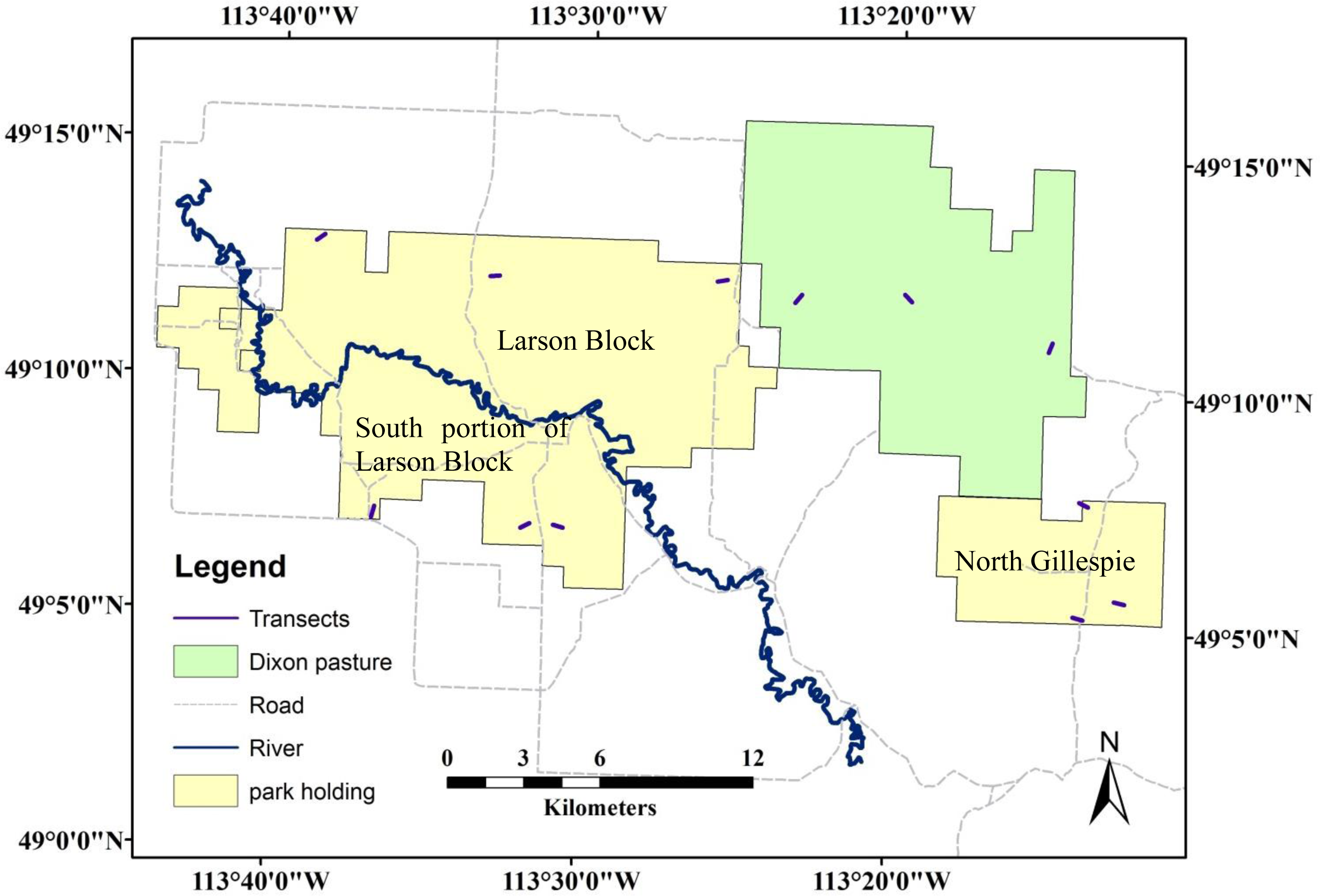
The study was conducted in GNP and the surrounding provincial community pastures in Saskatchewan, Canada (49°N, 107°W) (Figure 1). This area, located along the border with the United States of America, represents the northern extent of mixed grasslands. The park spans approximately 906 km² in area and incorporates two discontinuous blocks, the West Block and East Block (not shown in Figure 1). The climate of the region is semi-arid with approximately 350 mm of annual precipitation and 347 mm of annual evapotranspiration [14]. Three broad vegetation landscape units occur in the park: riparian shrubland, upland grassland, and valley grassland [15]. Upland grassland covers approximately two thirds of the park area. The dominant plant community in the uplands is needle and thread (Stipa comate Trin. and Rupr.), blue grama grass (Bouteloua gracilis (HBK) Lang. ex Steud.) and western wheatgrass (Pascopyrum smithii Rydb.). Valley grasslands are dominated by western wheatgrass and northern wheatgrass (Agropyron dasystachyum (Hook.) Scribn.) along with higher densities of shrubs and occasional trees. Common soil types in the park area are chernozemic (dark brown soil) and solonetzic soils (brown soil) [16]. Chernozemic soil is the most common in grassland communities with a dark color and high amount of organic content, and solonetzic soil has higher salinity and lighter color [8,17].

The park was established in 1984 and it was excluded from human disturbances, such as livestock grazing and prescribed burning, until 2005. Over nearly 30 years’ conservation, a large amount of senescence grasses have been accumulated. Although the surrounding pastures have been grazed, the grazing intensity was low and did not cause too much variation in terms of the percentage of dead material cover to the total land surface cover.

2.2. Sampling Design

The study was conducted in the West Block, including the southern portion of the Larson Block, the Larson and North Gillespie Blocks of GNP, and Dixon Provincial Community Pasture in 2008 (Figure 1). Among these regions, the southern portion of the Larson Block is excluded from grazing; the remaining three regions are grazed by large herbivores (bison and cattle). Grazing intensities in these sites are considered light to moderate. In each region, three long transects were established, formed by 128 quadrats, each 50 × 50 cm in size, and separated by a 3-m fixed interval. The location for each transect was predetermined by locating the study area with the Satellite Pour l’Observation de la Terre (SPOT) imagery acquired in June 2007 and a digital elevation model to make sure the transect was located in the upland grasslands to avoid the background variation caused by different soil types between upland and valley grasslands. In total, 12 transects were laid out. Each transect extended across the grazing pressure gradient from a water point to the upland, thus sampling areas of low and high dead materials, respectively.

2.3. Biophysical Data

Field work was conducted during the early growing season in 2008 from 20 May to 10 June. Within each quadrat, the percent cover of the following land-cover types were assessed visually: green grass, standing dead grasses, fallen litter, live forbs, live shrub, lichen, moss, bare ground and rock. After Daubenmire [18], the percentage of each quadrat covered by each land-cover type was first assigned to one of the six cover-classes: 0%–5%, 5%–25%, 25%–50%, 50%–75%, 75%–95%, and 95%–100%, then plant cover was further refined to the nearest 5% for cover values from 5% to 95% and to the nearest 1% for cover less than 5% and greater than 90%. The summed cover of standing dead grasses and fallen vegetation litter in each quadrat was used to represent the cover of dead material for that quadrat.

2.4. Remote Sensing Data

An ASD FieldSpec FR spectroradiometer (ASD, Boulder, CO, USA) was used to collect canopy reflectance data within each quadrat. The wavelength range is 350 nm to 2500 nm, with a spectral resolution of 1 nm. The canopy reflectance was collected with a fibre-optic tube having a 25° field of view (FOV) which corresponds to a FOV of approximately 1.5 m² with the spectroradiometer lens held approximately 1 m above the ground. All hyperspectral data were collected under clear-sky conditions within two hours of local solar noon. To reduce the atmospheric condition changes, the spectroradiometer was calibrated using a white spectral reference panel (Labsphere, Inc., North Sutton, NH, USA) at approximately 10-min intervals.

2.5. Vegetation Indices

Vegetation indices based on a combination of red and near-infrared wavelengths, or green, red, and near-infrared wavelengths were tested in this study (

Table 1. Vegetation indices tested in this study. The coefficients a (gain) and b (offset) in the equations for ATSAVI and L-ATSAVI are derived from the near-infrared vs. red rock–soil base line. In this study area a = 1.22 and b = 0.03 (X. Guo, unpublished data).

Vegetation Indices	Equation	Reference
SR (Simple Ratio Index)	$\frac{\rho 800}{\rho 670}$	[19]
NDVI (Normalized Difference Vegetation Index)	$\frac{\rho 800-\rho 670}{\rho 800+\rho 670}$	[20]
MSAVI (Modified Soil-Adjusted Vegetation Index)	$\frac{1}{2}\left[2\rho 800+1-\sqrt{{(2\rho 800+1)}^2-8(\rho 800-\rho 670)}\right]$	[26]
SAVI (Soil-Adjusted Vegetation Index)	$\frac{(1+L)(\rho 800-\rho 670)}{(\rho 800+\rho 670+L)}$	[24]
ATSAVI (Adjusted Transformed Soil-Adjusted Vegetation Index)	L = 0.5 $\frac{\alpha (\rho 800-\rho 670-b)}{\alpha \rho 800+\rho 670-ab+X(1+{\alpha }^2)}$	[25]
L-ATSAVI (Litter-Adjusted ATSAVI)	where X = 0.08 $\frac{\alpha (\rho 800-\alpha \rho 670-b)}{\alpha \rho 800+\rho 670-ab+X(1+{\alpha }^2)+L[0.5(\rho 2000+\rho 2200)-\rho 2100]}$	[1]
EVI (Enhanced Vegetation Index)	where X = 0.08 and L = 10 $\frac{2.5\times (\rho 800-\rho 670)}{L+\rho 800+c1\times \rho 670-c2\times \rho 550}$	[21]
WDVI (Weighted Difference Vegetation Index)	L = 1,C1 = 6.0,C2 = 7.5 ρ800 − α × ρ670	[22]
TVI (Triangular Vegetation Index)	60 × (ρ750 − ρ550) − 100(ρ670 − ρ550)	[27]

). The ratio-based indices of red and near-infrared bands [19–22], such as NDVI are some of the most widely used VIs available from different sensors with different spatial and temporal resolutions, such as the advanced very high resolution radiometer (AVHRR), moderate-resolution imaging spectroradiometer (MODIS), Landsat thematic mapper (TM) and Satellite Pour l’Observation de la Terre (SPOT) [23]. Soil-adjusted indices such as SAVI, TVI, MSAVI, and ATSAVI have been developed to minimize the soil background influence by using a soil line to characterize the soil spectra, and are useful in vegetation estimation in semi-arid systems where bare soil is exposed due to sparse vegetation [24–27]. L-ATSAVI was specifically designed for this study area; however, this index can be applied to other vegetated regions of a similar landscape. This index incorporates both the soil and dead material-adjusted factor in its definition. It is intended to perform well at estimating the green vegetation in a dead material dominant system [1].

2.6. Data Analysis

To test how the performance of vegetation indices was affected by various dead materials, the relationship between these two variables was examined using univariate regression analysis. Both linear and nonlinear models were applied in the regression analysis to fit the relationship. The model with high coefficient of determination (r²) was applied to describe the relationship between the dead material cover and VIs. Before conducting the regression analysis, all VIs and dead material cover data were pooled together. Vegetation indices were averaged for the quadrat with the same dead material cover. Dead material cover from different quadrats with same value was also averaged. On the basis of regression analysis, the sensitivities of the VIs to dead material cover were investigated using a sensitivity parameter(s) developed by Ji and Peters [28], which is defined as the ratio of the first derivative to the standard error of the regression function. Compared with current parameters for sensitivity analysis including goodness-of-fit measures (such as coefficient of determination (R²) and root mean squared error (RMSE) [29], relative equivalent noise (REN) [20], vegetation equivalent noise (VEN) [30,31], and relative sensitivity (Sr) [32], this new parameter not only indicates the sensitivity of the vegetation indices as a function of biophysical variables but also takes the estimation error of the regression function into account. Thus, it could express the sensitivity of the VIs comprehensively. The function of the parameter is defined as:

$$s=\frac{\widehat{y}}{{\sigma }_{\widehat{y}}}$$

(1)

where ŷ is a first derivative of the bivariate regression model using biophysical variables as independent variables (x) and each VI as the dependent variable (y). The fitted regression model is given by:

$$y=f(x)$$

(2)

and ŷ is expressed as:

$$\widehat{y}=f^{\prime }(x)=\frac{d(y)}{d(x)}$$

(3)

In linear and curvilinear regression function, σ_ŷ is given by:

$${\sigma }_{{\widehat{y}}_i}=\sqrt{{\sigma }^2{X^{\prime }}_i{\left(X^{\prime }X\right)}^{-1}{X}_i}$$

(4)

and for nonlinear regression function, σ_ŷ is given by:

$${\sigma }_{{\widehat{y}}_i}=\sqrt{{\sigma }^2{F^{\prime }}_i{\left(F^{\prime }F\right)}^{-1}{F}_i}$$

(5)

where σ² is the mean square error, X is the matrix of independent variables, and X_i is the ith row of X, F is the matrix of derivatives for approximating least squares estimations and F_i denotes the ith row of F matrix [33]. Student’s t-test was applied to test the significance of ŷ, and p < 0.05 was used to determine the significance.

3. Results

3.1. Mixed Grassland Biophysical Characteristics

In the study area, dead materials were a major component of the vegetation canopy while green grass, which ranked second, provided a relatively small proportion (

Table 2. Descriptive statistics of biophysical variables of mixed grasslands. STD stands for standard deviation; CV stands for coefficient of Variance and N stands for sample size.

Value	Canopy Cover (%)
	Green Grass	Forb	Shrub	Dead Materials	Moss	Lichen	Bare Ground	Rock
Mean	8.8	2.4	2.8	66.7	8.1	5.7	2.9	2.7
Median	8	1	0	69	8	2	0	0
Min	0	0	0	4.0	0	0	0	0
Max	50	30	35	100	35	60	70	74
STD	5.7	3.5	5.2	15.9	8.1	8.0	7.9	6.7
CV	1.5	0.7	0.5	4.2	1.0	0.7	0.4	0.4
N	1536	1536	1536	1536	1536	1536	1536	1536

). Dead materials covered about of 69% of ground surface. The cover of green grass was 8%. Dead materials together with green grass constituted almost 77% of the canopy cover. Unlike most of the semi-arid grassland ecosystems, the bare ground and rock in the study area were relatively small with the median value of 0%.

3.2. Spectral Features of Mixed Grasslands

The characteristics of vegetation composition affect its spectral response. Figure 2 showed the reflectance spectra of mixed grasslands in the study area. The spectral curve was the average of reflectance from all quadrats. The spectral reflectance curve showed an increasing trend from the blue to the green wavelength region, relatively stable between the green and red wavelength regions and high reflectance in the near-infrared and mid-infrared regions.

3.3. Relationship between Dead Material Cover and Vegetation Indices

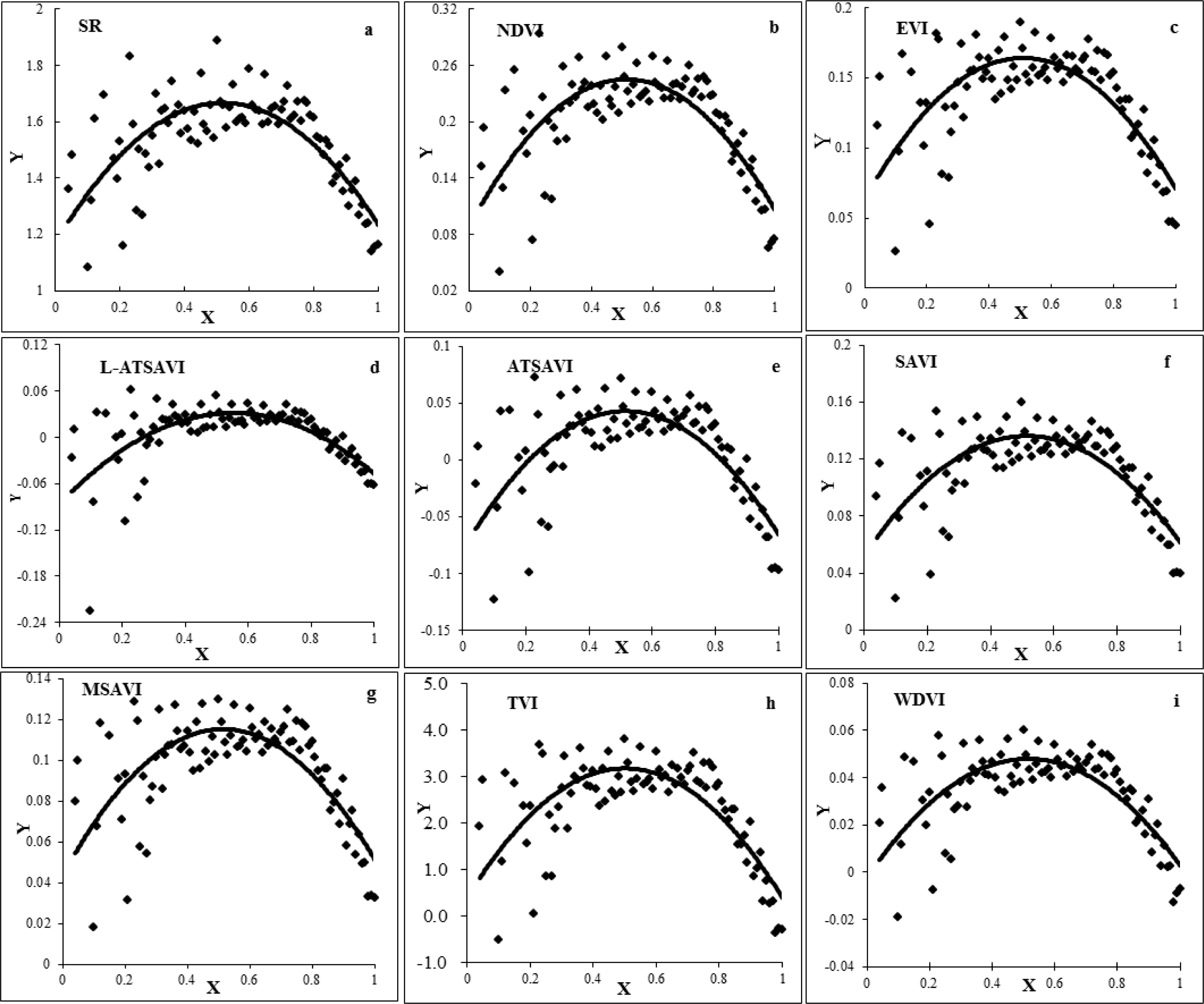
The quadratic model was found best fitting the relationship between dead material cover and VIs (Figure 3 and

Table 3. Summary statistics for the relationships between VIs and dead material cover.

Vegetation Indices	Equation	R2	df(y)/df(x)	Dead Material Cover with df(y)/df(x) = 0
SR	Y = −1.85x2 + 1.92x + 1.17	0.56	0	50%
NDVI	Y = −0.59x2 + 0.61x + 0.09	0.56	0	50%
ATSAVI	Y = −0.46x2 + 0.47x − 0.08	0.54	0	48%
L-ATSAVI	Y = −0.39x2 + 0.43x − 0.09	0.40	0	56%
SAVI	Y = −0.32x2 + 0.33x + 0.05	0.53	0	55%
EVI	Y = −0.38x2 + 0.4x + 0.06	0.53	0	50%
WDVI	Y = −0.19x2 + 0.2x − 0.002	0.54	0	50%
MSAVI	Y = −0.27x2 + 0.28x + 0.04	0.53	0	45%
TVI	Y = −11.13x2 + 11.13 + 0.38	0.56	0	50%

). According to the r² values (Table 3), NDVI, SR and TVI showed a slightly higher correlation with dead material cover, and the performances of soil-adjusted indices (ATSAVI, SAVI, MSAVI) and WDVI were all similar. Among all VIs, L-ATSAVI had the lowest correlation with dead material cover. Overall, the quadratic model indicated that at lower level of dead material cover (<30%), positive relationships were evident between VIs and the dead material cover. At mid dead material cover levels (30%–60%), the VIs were not sensitive to changes in dead material cover; and where the dead material cover exceeds 60%, negative relationships were evident (Figure 3).

The quadratic relationship (Figure 3) cannot be applied to estimate the cover of dead materials from VIs. Therefore, we split the dataset into two groups to fit linear regressions. For each VI tested, the breakpoint of the dataset was determined as the graph (Figure 3) where slope was zero. The changes in slopes of the developed models reflect the changes in relationships between VIs and dead material cover. The corresponding dead material cover where the slope of the model developed for each VI turns to zero was used as the breakpoint. The breakpoints for most VIs were 50% and the rest were around 50% (Table 3). Applying different breakpoints to VIs caused different dataset size among VIs. To avoid the effect of different dataset sizes on model fit and sensitivity among VIs, 50% dead material cover was used as the breakpoint of dataset for all VIs to make sure that they all had the same dataset size.

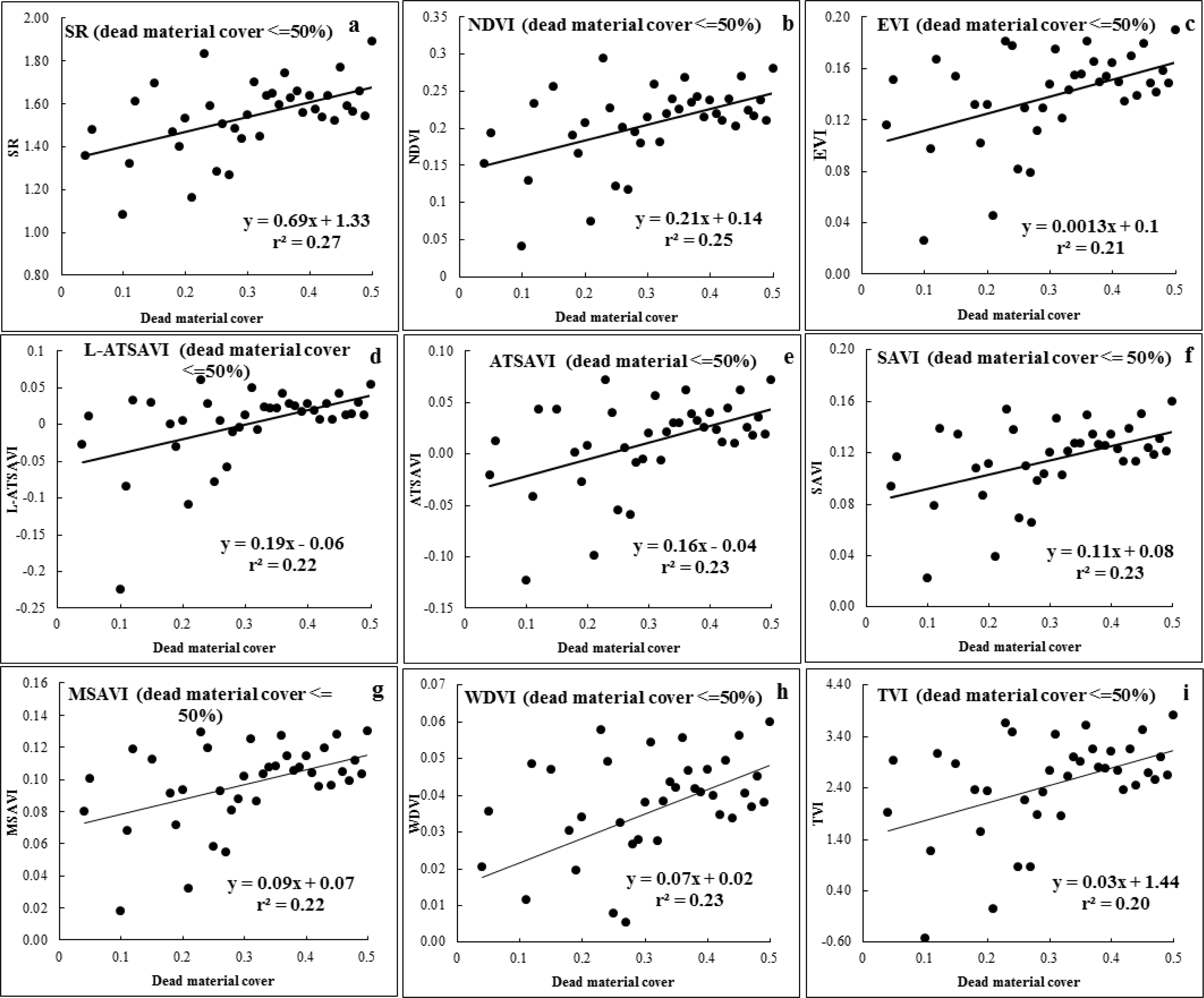
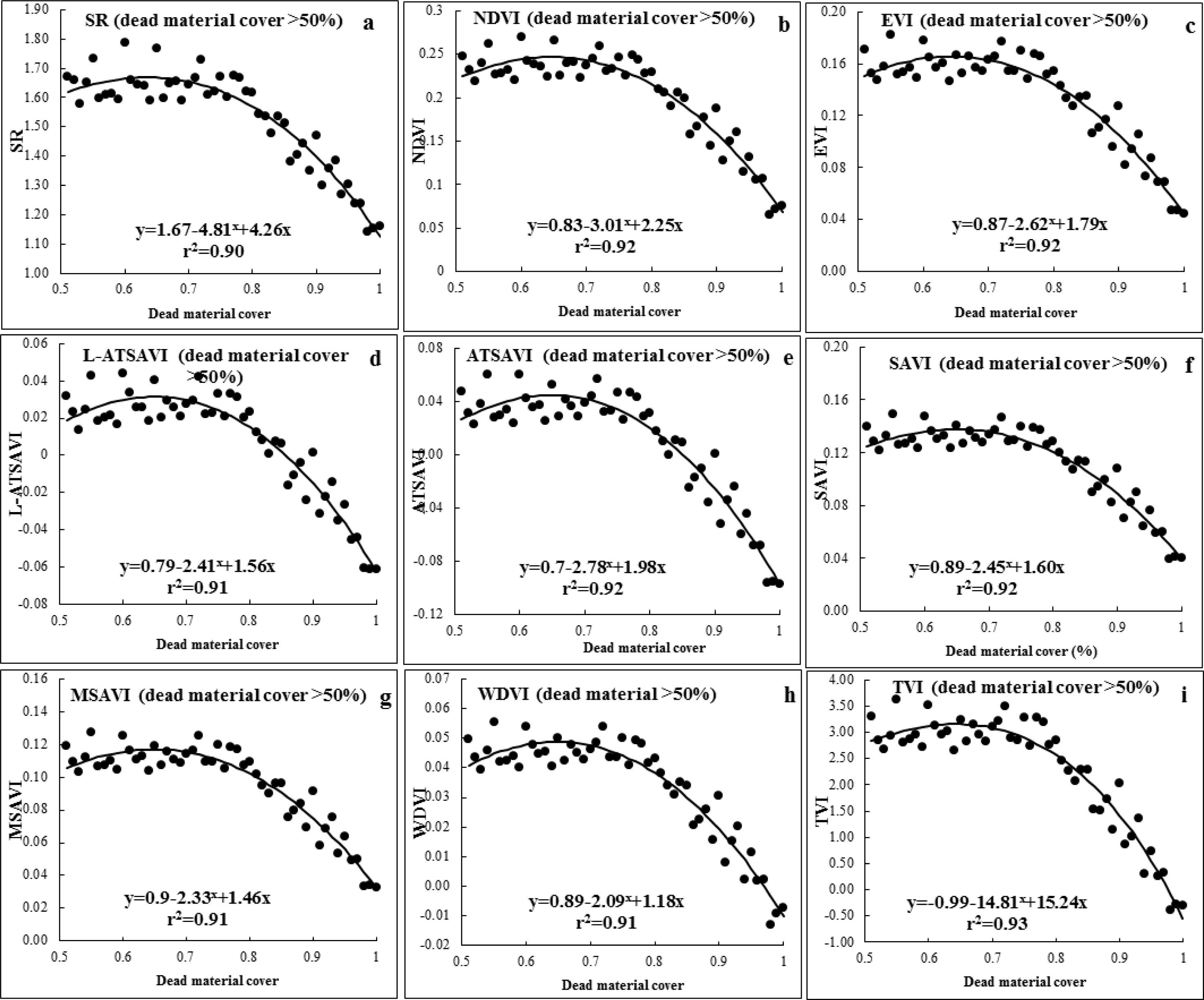
After the dataset was divided into two groups, regression analysis was applied to each of them separately to re-evaluate the relationship between VIs and dead material cover. Using this segmented regression analysis, we found that the relationship was positive (but weak) with less than 50% cover of dead material (Figure 4) but negative where the cover was greater than 50% (Figure 5). A combined exponential and linear model best fitted the relationship between VIs and dead material cover that was greater than 50%, with r² higher than 0.90 (Figure 5).

3.4. Sensitivity of the Vegetation Indices

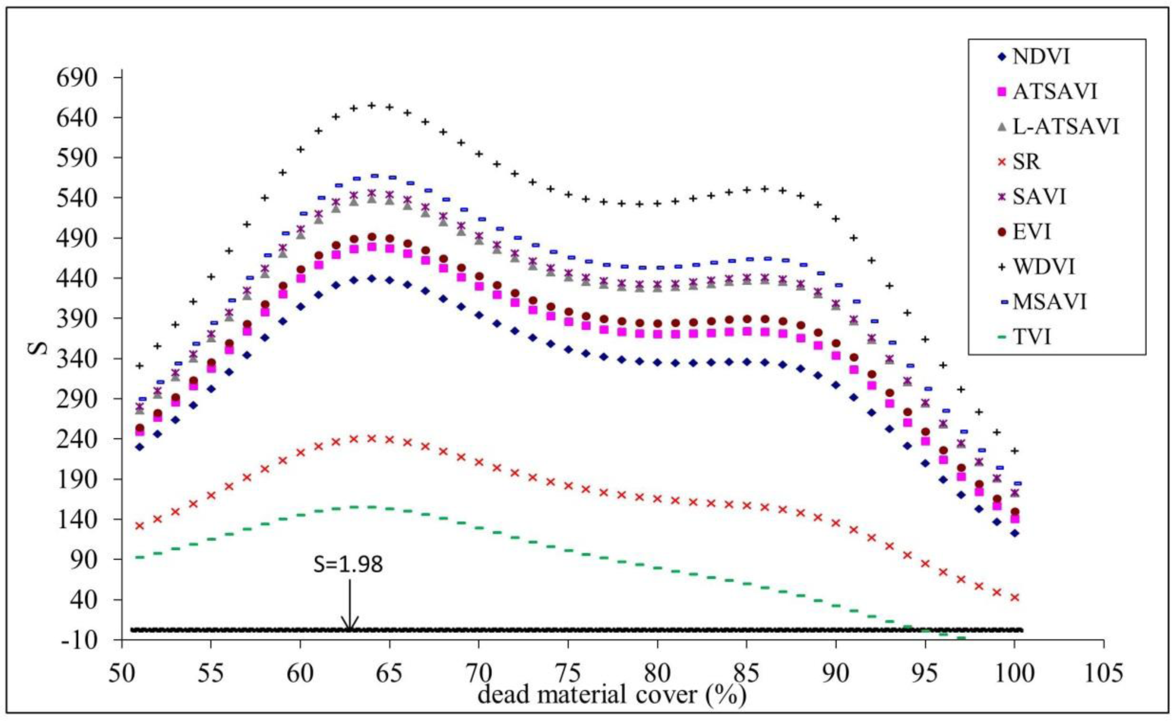
A sensitivity analysis was conducted to further investigate how sensitive each VI is to a change in dead material cover higher than 50% as shown in Figure 6. A relatively high sensitivity was found for VIs when dead material cover was >60% and <90% except TVI and SR which had higher sensitivity when dead material cover was >60% and <70%. Among the nine VIs, WDVI had the highest sensitivity over the entire range of dead material cover. The sensitivities of TVI and SR were relatively low compared to the remaining VIs. T-statistics indicated that the t-scores (same as s values) were all greater than 1.98 for the nine VIs, except TVI, which had an s-value less than 1.98 when dead material cover was >94%. In this analysis, 1.98 is the critical value in a two-tailed t-test (α = 0.05, degree of freedom (df) = 48) for rejecting the null hypothesis. Thus we concluded that all VIs were significantly sensitive to dead material cover, except TVI, which was not significant when dead material cover was greater than 94%.

4. Discussion

Changes in the condition and composition of vegetation lead to changes in the spectral signature of the land surface. Dead materials are a major component of the study area. With the amount of dead materials accumulated, the vegetation spectral curve of the study area showed increasing reflectance in blue, red and mid-infrared wavelength regions and decreasing reflectance in the near-infrared wavelength region, compared to the abundant closed green vegetation canopies. The reflectance in the visible region of the spectrum (0.35–0.7 μm) is primarily a function of vegetation density (for example, biomass per unit) and of the chlorophyll content of the leaves [34]. For our case, the increases of reflectance in blue and red regions were more likely due to the reduced chlorophyll content of dead materials. The decrease in reflectance of near-infrared and increase in mid-infrared were potentially attributed to the larger intercellular space and less water content of dead materials when compared with green vegetation [35]. The spectral signature of the study area illustrated that dead materials were one of the major surface components controlling the spectral behavior of vegetation canopies.

The linear relationship between VIs and vegetation properties has been reported in previous studies [8,9,36]; however, we found the responses of VIs were not consistent along the whole range of dead material cover. As indicated by Van Leeuwen and Huete [31] the variability among, and the differences between, the spectral properties of dead materials, green vegetation and soil determined whether the vegetation index response increases or decreases. The weak relationships between VIs and dead material cover that is less than 50% may be attributed to the confounding effects of soil background. Previous studies [11,37] have indicated the poor performance of Red-NIR based vegetation indices for discriminating dead materials due to the similar spectral features of dead materials and soil at VIS-NIR wavelength ranges [38]. As dead materials increase and cover the majority of land surface, the effects of soil are much less than at low dead material covers. Significant relationships between VIs and dead material cover were found when dead material cover was higher than 50%, which suggested their suitability for estimating the cover of dead material.

The sensitivity analysis which tracks the sensitivities of VIs through the range of dead material cover provides more detailed information on VIs’s performance. Although VIs have similar r², their sensitivity varied with the WDVI having the highest sensitivity over the entire range of dead material cover. The insignificant sensitivity of TVI in dead material cover higher than 94% implied that TVI was not suitable for predicting dead material cover with high density (for example >94%). By just focusing on the dead material cover with high density (>50%), the performance of VIs on estimation of dead material cover in terms of r² (>0.9) was dramatically improved compared to previous studies [8,38]. For example, Zhang et al. [8] reported the correlation coefficients (r) between dead grass cover with VIs derived from SPOT 5 images including NDVI, AISAVI, normalized cover index (NDCI) and ratio cover index (RCI) ranged from 0.47 to 0.56, which equal to r² of 0.22 to 0.30. Daughtry et al. [37] reported an r² of 0.89 when relating crop residue to the cellulose absorption index (CAI), an index based on narrow bands, which was designed for quantification of senescent grass cover [13].

5. Conclusions

Understanding the responses of commonly used VIs to dead material cover in mixed grassland is essential for quantifying green vegetation biophysical properties as the dead material is one of the major vegetation components in this area which confounds the spectral feature of green vegetation. Results from this study indicated that the responses of VIs tested in this study were not consistent along the whole range of dead material cover. VIs tested in this study could be used for estimating dead material cover that is greater than 50% in mixed grasslands. WDVI, which has the highest sensitivity and similar r² to the remaining Vis, provided the best performance for estimation of dead materials cover higher than 50%, among VIs tested in this study. The VIs selected for this study were primarily based on red and near-infrared bands and limited for estimation of dead material cover with high density (>50%). VIs based on other wavelength regions (for example, mid-infrared wavelength) are worthy of being tested using the methods applied in this study in future work.

References

- He, Y.; Guo, X.; Wilmshurst, J.F. Studying mixed grassland ecosystem I: Suitable hyperspectral vegetation indices. Can. J. Remote Sens 2006, 32, 98–107. [Google Scholar]
- Paruelo, J.M.; Epstein, H.E.; Lauenroth, W.K.; Burke, I.C. ANNP estimations from NDVI for the central grassland region of the United States. Ecology 1997, 7, 953–958. [Google Scholar]
- Purevdorj, T.; Tateishi, R.; Ishiyama, T.; Honda, Y. Relationship between percent vegetation cover and vegetation indices. Int. J. Remote Sens 1998, 19, 3519–3535. [Google Scholar]
- Moreau, S.; Bosseno, R.; Gu, X.F.; Baret, F. Assessing the biomass dynamic of Andean bofedal and totora high-protein wetland grasses from NOAA/AVHRR. Remote Sens. Environ 2003, 85, 516–529. [Google Scholar]
- Jackson, R.D.; Huete, A.R. Interpreting vegetation indices. Prebentive Vet. Med 1991, 11, 185–200. [Google Scholar]
- Pickup, G.; Chewings, V.H.; Nelson, D.J. Estimating changes in vegetation cover over time in arid rangelands using Landsat MSS data. Remote Sens. Environ 1993, 43, 243–263. [Google Scholar]
- Guo, X.; Zhang, C.; Wilmshurst, J.F.; Sissons, R. Monitoring grassland health with remote sensing approaches. Prairie Perspect 2005, 8, 11–22. [Google Scholar]
- Zhang, C.; Guo, X. Monitoring northern mixed prairie health using broadband satellite imagery. Int. J. Remote Sens 2008, 29, 2257–2271. [Google Scholar]
- Yang, X.; Guo, X.; Fitzsimmons, M. Assessing light to moderate grazing effects on grassland production using satellite imagery. Int. J. Remote Sens 2012, 33, 5087–5104. [Google Scholar]
- Frank, A.B.; Aase, J.K. Residue effects on radiometric reflectance measurements of Northern Great Plains rangelands. Remote Sens. Environ 1994, 49, 195–199. [Google Scholar]
- Daughtry, C.S.T.; McMurtrey, J.E., III; Nagler, P.L.; Kim, M.S.; Chappelle, E.W. Spectral Reflectance of Soil and Crop Residues. In Near Infrared Spectroscopy: The Future Waves; Davies, A.M.C., Williams, P., Eds.; NIR Publications: Chichester, UK, 1996; pp. 505–511. [Google Scholar]
- Goward, S.N.; Huemmrich, K.F. Vgetation canopy PAR absorptance and the normalized difference vegetation index: An assessment using the SAIL model. Remote Sens. Environ 1991, 39, 119–140. [Google Scholar]
- Nagler, P.L.; Daughtry, C.S.T.; Goward, S.N. Plant litter and soil reflectance. Remote Sens. Environ 2000, 71, 207–215. [Google Scholar]
- Environment Canada, 2003 Canadian Climate Normals or Average 1971–2000. Available online: http://www.climate.weatheroffice.ec.gc.ca/climate_normals/index_e.html(accessed on 24 August 2009).
- Michalsky, S.J.; Ellise, R.A. Vegetation of Grasslands National Parks; D.A. Westworth and Associates Ltd.: Calgary, AB, Canada, 1994. [Google Scholar]
- Fargey, K.S.; Larson, S.D.; Grant, S.J.; Fargey, P.; Schmidt, C. Grasslands National Park Field Guide; Prairie Wind and Silver Sage—Friends of Grasslands Inc.: Val Marie, SK, Canada, 2000. [Google Scholar]
- Zhang, C.; Guo, X. Measuring biological heterogeneity in the northern mixed prairie: A remote sensing approach. Can. Geogr 2007, 51, 462–474. [Google Scholar]
- Daubenmier, R. A canopy-coverage method of vegetational analysis. Northwest. Sci 1959, 33, 43–64. [Google Scholar]
- Jordan, C.F. Derivation of leaf area index from quality of light on the first floor. Ecology 1969, 50, 663–666. [Google Scholar]
- Rouse, J.W.; Haas, R.H.; Schell, J.A.; Deering, D.W.; Harlan, J.C. Monitoring the Vernal Advancement of Retrogradation of Natural Vegetation. In Type III, Final Report; National Aeronautics and Space Administration, Goddard Space Flight Centre (NASA/GSFC): Greenbelt, MD, USA, 1974; p. 371. [Google Scholar]
- Liu, H.Q.; Huete, A.R. A feedback based modification of the NDVI to minimize canopy background and atmospheric noise. IEEE Trans. Geosci. Remote Sens 1995, 33, 457–465. [Google Scholar]
- Clevers, J.C.P.W. The application of a weighted infrared-red vegetation index for estimating leaf area index by correcting for soil moisture. Remote Sens. Environ 1989, 29, 25–37. [Google Scholar]
- Petoorelli, N.; Vik, J.O.; Mysterud, A.; Gaillard, J.; Tucker, C.J.; Stenseth, N.C. Using the satellite–derived NDVI to assess ecological responses to environmental change. Trends Ecol. Evol 2005, 20, 503–510. [Google Scholar]
- Huete, A.R. A soil-adjusted vegetation index (SAVI). Remote Sens. Environ 1988, 25, 295–309. [Google Scholar]
- Baret, F.; Guyot, G. Potential and limits of vegetation indices for LAI and APAR assessment. Remote Sens. Environ 1991, 35, 161–173. [Google Scholar]
- Qi, J.; Chehbouni, A.; Huete, A.R.; Kerr, Y.H.; Sorooshian, S. A modified soil adjusted vegetation index. Remote Sens. Environ 1994, 48, 119–126. [Google Scholar]
- Broge, N.H.; Leblanc, E. Comparing prediction power and stability of broadband and hyperspectral vegetation indices for estimation of green leaf area index and canopy chlorophyll density. Remote Sens. Environ 2000, 76, 156–172. [Google Scholar]
- Ji, L.; Peters, A.J. Performance evaluation of spectral vegetation indices using a statistical sensitivity function. Remote Sens. Environ 2007, 106, 59–65. [Google Scholar]
- Yang, X.; Kovach, E.; Guo, X. Biophysical and spectral responses to various burn treatments in the northern mixed-grass prairie. Can. J. Remote Sens 2013, 39, 175–184. [Google Scholar]
- Huete, A.; Justice, C.; Liu, H. Development of vegetation and soil indices for MODIS-EOS. Remote Sens. Environ 1994, 49, 224–234. [Google Scholar]
- Van Leeuwen, W.J.D.; Huete, A.R. Effects of standing litter on the biophysical interpretation of plant canopies with spectral indices. Remote Sens. Environ 1996, 55, 123–138. [Google Scholar]
- Gitelson, A.A. Wide dynamic range vegetation index for remote quantification of biophysical characteristics of vegetation. J. Plant Physiol 2003, 161, 165–173. [Google Scholar]
- Schabenberger, O.; Pierce, F.J. Contemporary Statistical Models for the Plant and Soil Sciences; CRC Press: Boca Raton, FL, USA, 2002; p. 738. [Google Scholar]
- Woolley, J.T. Reflectance and transmittance of light by leaves. Plant Physiol 1971, 47, 656–662. [Google Scholar]
- Paltridge, G.W.; Barber, J. Monitoring grassland dryness and fire potential in Australia with NOAA/AVHRR data. Remote Sens. Environ 1988, 25, 381–394. [Google Scholar]
- Aase, J.K.; Tanaka, D.L. Reflectance from four wheat residue cover sensitivities as influenced by three soil background. Agron. J 1991, 83, 753–757. [Google Scholar]
- Daughtry, C.S.T.; Hunt, E.; McMurtrey, J.E., III. Assessing crop residue cover using shortwave infrared reflectance. Remote Sens. Environ 2004, 90, 126–134. [Google Scholar]
- Wiegand, C.L.; Richardson, A.J. Relating spectral observations of the agricultural landscape to crop yield. Food Struct 1992, 11, 249–258. [Google Scholar]