Transferability of a Visible and Near-Infrared Model for Soil Organic Matter Estimation in Riparian Landscapes

 ,
, 
Abstract
: The transferability of a visible and near-infrared (VNIR) model for soil organic matter (SOM) estimation in riparian landscapes is explored. The results indicate that for the soil samples with air-drying, grinding and 2-mm sieving pretreatment, the model calibrated from the soil sample set with mixed land-use types can be applied in the SOM prediction of cropland soil samples (r2Pre = 0.66, RMSE = 2.78 g·kg−1, residual prediction deviation (RPD) = 1.45). The models calibrated from cropland soil samples, however, cannot be transferred to the SOM prediction of soil samples with diverse land-use types and different SOM ranges. Wavelengths in the region of 350–800 nm and around 1900 nm are important for SOM estimation. The correlation analysis reveals that the spectral wavelengths from the soil samples with and without the air-drying, grinding and 2-mm sieving pretreatment are not linearly correlated at each wavelength in the region of 350–1000 nm, which is an important spectral region for SOM estimation in riparian landscapes. This result explains why the models calibrated from samples without pretreatment fail in the SOM estimation. The Kennard–Stone algorithm performed well in the selection of a representative subset for SOM estimation using the spectra of soil samples with pretreatment, but failed in soil samples without the pretreatment. Our study also demonstrates that a widely applicable SOM prediction model for riparian landscapes should be based on a wide range of SOM content.1. Introduction
Soil organic matter (SOM) content is a key soil property in soil surveying, because of its important role in the global carbon cycle, precise agricultural management and soil erosion evaluation [1–3]. In riparian landscapes, SOM is also considered as an important indicator for soil quality, because of its relationship with critical soil functions, such as productivity, erodibility and purification ability [4]. In spite of their important roles in geomorphology and hydrology, many of the riparian zones in the population-dense areas of China are suffering from the adverse impacts of agricultural practices [5,6]. Thus, it is necessary to monitor the spatial and temporal dynamics of SOM for a better management of the land resources in riparian landscapes.
Conventional measurements of organic matter in soil still require time-consuming field sampling and intensive laboratory work, which could be costly [7,8]. Visible and near-infrared (VNIR) spectroscopy, which began to take off around the year 2008 [9], provides an alternative to SOM measurement in the laboratory [10], as well as in the field [11,12]. It has proven to be a rapid and efficient technique for estimating a variety of soil properties, including the SOM content [3,13,14]. The prediction accuracies of the VNIR models for SOM content have, however, varied from less than satisfactory [15] to satisfactory [16], depending on the land use [7], the source of the VNIR data, the calibration methods, scanning environments, soil chromophores (e.g., iron oxide) and even the spectroscopic instruments [10,11,13,17]. The mechanisms for the VNIR estimation of SOM content are its broad absorptions in the visible region, due to chromophores and the darkness of humic acid, and the absorptions in the NIR region from the overtones of O-H, C-H and N-H, or their combination [13,18].
Although there have been extensive studies of the VNIR estimation of SOM content, it is generally agreed that most of the models are location-dependent and data-specific [13,19,20]. A frequently asked question by the potential users of VNIR models for SOM estimation is: will a model calibrated from samples in a certain location work in other locations? When referring to other locations, the soil parent materials, range of SOM content, land use and land cover could be different. It has been revealed that the transferability of a VNIR model depended on whether or not the calibrations contained the variability of the target site soil [20]. In order to take full advantage of the VNIR spectroscopy for soil characterization, it would be desirable to minimize the number of calibration samples [21]. Recent efforts have been made for better predictions of soil properties, with the assistance of soil spectral libraries at continental [7], national [21,22], regional [23] and local scales [22]. Nevertheless, it remains a challenge to develop an effective strategy for the VNIR estimation of SOM when the local soil spectral libraries are unavailable and in the areas where the soils are largely influenced by human activities. Hence, it is essential to carry out a study concerning the VNIR estimation of SOM content with samples from different locations with different land-use types and a range of SOM content.
Moreover, most of the previous studies have focused more on the laboratory measurement of air-dried, ground and sieved soil samples using VNIR spectroscopy [24]. Very few of the studies have explored the relationship between the spectra from soil samples with different pretreatments at each single wavelength. The feasibility of the VNIR estimation of soil properties with different sample pretreatments and spectral transformations has not been fully studied. Such studies are both important and necessary because of the recent migration of the VNIR estimation of soil properties from laboratory to in situ applications [25]. Thus, a case study implementing correlation analysis is essential to provide a statistical inspection of the effects of soil sample preparation and spectral transformations.
The aim of this paper is to explore the transferability of several VNIR models for SOM estimation in riparian landscapes, where quick and easy access to SOM data is becoming an increasingly important concern for the sustainable use of land resources. Several sample division strategies have been used to achieve our goal: training and test sets divided by sample locations and land-use types, SOM content and the Euclidean distance of soil spectra (using the Kennard–Stone algorithm). Reflectance and absorbance from soil samples with and without air-drying, grinding and 2 mm-sieving pretreatment have been used in our study. Besides, we explore the relationship between the spectra from soil samples with different pretreatments at each single wavelength and compare the suitability of the proposed sample division strategies for an accurate estimation of SOM content with spectra from differently pretreated soils.
2. Material and Methods
In this section, we confirm that the owner of the land gave permission for us to conduct the study on this site. The field studies did not involve endangered or protected species.
2.1. Description of the Study Area
The study area is located in the Honghu City area (Hubei Province) in the Jianghan plain (Figure 1), which is a core food production area in Hubei Province, with a sown area of grain reaching 884 km2 and a total grain production of 670 thousand tons in the year 2012, increasing by 9.2% and 2.2%, respectively, in comparison with the year 2011 (according to the report by the Ministry of Agriculture of the People’s Republic of China, http://www.moa.gov.cn/). The Honghu City area is also known for its riparian landscape, as well as the dramatic changes in terms of land use and land cover since the 1950s [26]. Ecological concerns have been recently raised because of the ever-increasing impact that human activities exert on the environment in this area [27,28].
The landform of the study area is flat, with an average elevation of below 50 m. Inceptisols dominate the study area, according to USDA soil taxonomy. Water bodies, lacustrine vegetation, floodplain, cropland and open land are the major land-cover types [29]. According to the field survey conducted in December 2011, artificial forest and meadow are also now important components of the land-cover types in this region. Paddy field and irrigated cropland are the major land-use types of the cropland areas.
2.2. Field Sampling
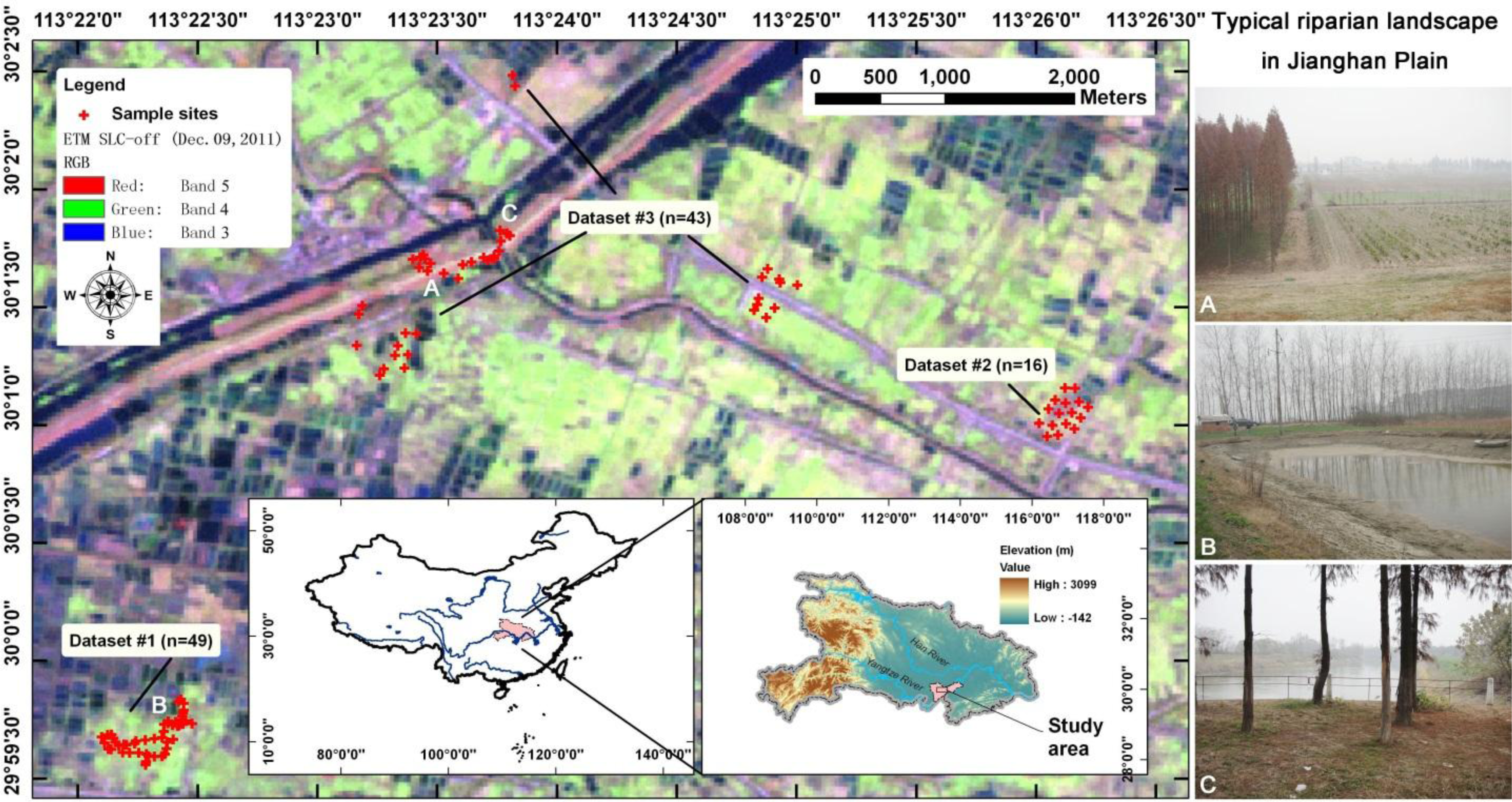
From 20 December 2011 to 21 December 2011, with the permission of the local residents, a total of 108 top-layer (0–15 cm) soil samples were collected in the study area. Figure 1 shows the spatial distribution of the sample sites, with a false-color composite Enhanced Thematic Mapper (ETM) image (RGB corresponding to Band 5, Band 4 and Band 3, respectively) showing the landscape of the study area. The spectral range of Band 5 is 1.55–1.75 μm; Band 4 is 0.76–0.90 μm, and Band 3 is 0.63–0.69 μm. The vegetated areas therefore show as green, while the water bodies (e.g., breeding ponds) appear to be blue. The total set of the soil samples (Dataset 0, n = 108) was divided into three subsets by the land-use types and locations, namely Dataset 1 (n = 49), Dataset 2 (n = 16) and Dataset 3 (n = 43). The first two datasets were from cropland. As the study was conducted in winter, further classification of the cropland into paddy field and irrigated cropland was not made. It should be noted that Dataset 1 was much closer to the breeding pond area, while Dataset 2 was surrounded by cropland. Differing significantly from Dataset 1 and Dataset 2, Dataset 3 covered a larger geographical region and mixed land-use types, including cropland covered by a variety of vegetation, artificial forest, meadows and breeding ponds. The samples of the breeding ponds were collected from surface sediment. The minimum distance between each sampling site was approximately 20 m. The fine sampling density of the cropland was subject to the high spatial heterogeneity of SOM [30], as well as the diverse management practices, land use and land cover identified in the field survey. The geographical coordinates were recorded by a hand-held global positioning system (GPS) with a positional error of <5 m. All the soil samples were taken to the laboratory on 22 December 2011.
2.3. Laboratory VNIR Reflectance Analyses
In order to examine the relationship between the spectra from soil samples with different pretreatments at each single wavelength, the reflectance of the soil samples was measured from soil samples with and without the air-drying, grinding and 2-mm sieving pretreatment [13,31].
An ASD FieldSpec 3 portable spectroradiometer with a wavelength of 350–2500 nm was used to measure the reflectance of the soil samples. The sampling interval and spectral resolution were 1.4 nm and 3 nm for the 350–1000 nm range and 2 nm and 10 nm for the 1000–2500 nm range ( http://www.asdi.com). A standardized white Spectralon® panel was used for the reflectance calibration. A white light source matched with the spectroradiometer was used with a 45° incidence angle. A soil sample of around 300 g, spanning a diameter of approximately 20 cm and a sample depth of approximately 10 mm, was scanned by the spectroradiometer, with a distance of 12 cm from the probe to the sample surface and a zenith angle of 90°. The whole scanning procedure was carried out in a dark room at night, minimizing the influence of external light.
Two spectral datasets were obtained after the laboratory VNIR reflectance analyses. Spectra from the soil samples with the air-drying, grinding and 2-mm sieving pretreatment were denoted as AP. The spectra from the samples without pretreatment were denoted as BP.
2.4. Chemical Analyses of Soil Properties
The SOM content of all the 108 soil samples was measured by wet oxidation at 180 °C with a mixture of potassium dichromate and sulfuric acid [32].
2.5. Spectral Pre-Processing
Spectral pre-processing is essential in chemometrics modeling and can largely eliminate the baseline shift and non-linearities [33]. For the VNIR estimation of SOM content, transformations, such as absorbance (log 1/R, R = reflectance), are wildly used [34,35]. MATLAB® (R2008a, MathWorks, Inc.) was used here to transform the reflectance to absorbance.
2.6. Statistical Analyses
Statistical analyses, including descriptive statistics, histograms, box plots and Pearson correlation analyses were implemented using MATLAB® (R2008a). The Pearson correlation coefficient was used to assess the relationships between: (1) the spectra and the SOM content, with a confidence level of 99.999% (two-tailed); (2) wavelength pairs (e.g., spectra at 380 nm and spectra at 800 nm) of reflectance from different soil sample sets; and (3) the spectra at a specific wavelength from soil samples without preparation and the spectra at the same wavelength from the pretreated samples.
2.7. PLSR Modeling of Soil Organic Matter
Nine modeling schemes were designed to fulfill the objectives of this study. Scheme 1 was designed to examine the transferability of the VNIR model for SOM estimation with soil samples from the same land-use type, but from different plots with different data ranges of SOM content. The total sample set (Dataset 0) was split into a training set with 49 samples from cropland in one plot (Dataset 1) and a test set with 16 samples from cropland in another plot (Dataset 2). With soil samples from different land-use types forming Dataset 3, Scheme 2 to Scheme 6 employed this dataset as a training set or a test set to answer the question of “whether the VNIR model for SOM estimation calibrated for one subset of land use can be transferred to other classes without further calibration”.
In addition to the division of the total sample set (Dataset 0) into three subsets by geographical location, Dataset 0 was divided into two sets (Dataset D and Dataset S) of 54 samples each, according to the sorting of the SOM content. Dataset 0 was first sorted in ascending order, then Dataset D was formed from the odd samples and Dataset S was formed from the even samples. It was assumed that such a process would ensure a relatively equal distribution of the samples of different land-use types and a similar range of SOM content. With Dataset D (or Dataset S) as the training set and Dataset S (or Dataset D) as the test set, Scheme 7 (or Scheme 8) was designed to evaluate the general predictive capacity of the VNIR model for SOM estimation, regardless of the land-use type and the geographical location of the samples.
Scheme 9, with the training set (Dataset KSc) and test set (Dataset KSp) divided by the Kennard–Stone algorithm [36,37], was used to examine the research question of whether half of the total samples selected according to their spectral differences could be representative enough to calibrate a successful model for predicting the SOM content of the remaining samples. By computing the Euclidean distances on full spectra (350–2500 nm) between all pairwise spectra of soil samples, the Kennard–Stone algorithm first selected the two samples farthest apart from each other. The third sample selected was the one farthest from the first two. The selection process continued, until 54 samples (50% of the total sample set) were selected. These selected samples were used as training set (Dataset KSc), while the remaining 54 samples were used as test set (Dataset KSp). The Kennard–Stone algorithm has been regarded as an effective method for the selection of a representative subset in the VNIR modeling of soil properties [7,22,37]. This algorithm, however, has seldom been applied using spectra from soil samples without air-drying, grinding and 2-mm sieving pretreatment. Therefore, it is necessary to examine its performance in soils with different pretreatments.
PLSR coupled with leave-one-out cross-validation was used to relate the two spectral datasets BP and AP (explanatory variables) to the SOM content (response variable). PLSR is a routine modeling technique used for quantitative spectral analysis and is particularly useful when dealing with highly correlated predictor variables whose number is much larger than that of the samples [17,38]. The PLSR projects explanatory variables (spectral data) and response variable (SOM content) into a low-dimensional space, maximizing the covariance between the scores of the explanatory variables and response variable. The PLSR method can be implemented in a variety of software packages, such as ParLeS [39] and The Unscrambler ( http://www.camo.com/). Thus, the algorithm is not introduced here, but can be referred to in a number of previous studies [38,40]. This study used the PLS toolbox (Version 6.7.1) from Eigenvector Research, Inc. (Wenatchee, WA, USA), which is MATLAB-based software. Leave-one-out cross-validation was used to decide the optimal number of factors retained in the calibration models by minimization of the root mean square error (RMSE) for the cross-validation (RMSECV). Variable importance in the projection (VIP), with a threshold of 1, was used to determine the important wavelengths used in the PLSR calibration [13,41,42].
Two validation strategies, namely leave-one-out cross-validation and external validation using an independent dataset, were adopted to examine the model performance. Residual prediction deviation (RPD), along with the coefficient of determination (r2) and the RMSE for the cross-validation (r2cv, RMSECV) and prediction (r2Pre, RMSEP), were computed to interpret the model predictive ability [42,43]. For the VNIR estimation of the soil properties, RPD > 1.4 indicates an acceptable predictive ability for the model [43].
3. Results and Discussion
3.1. Sample Characterization
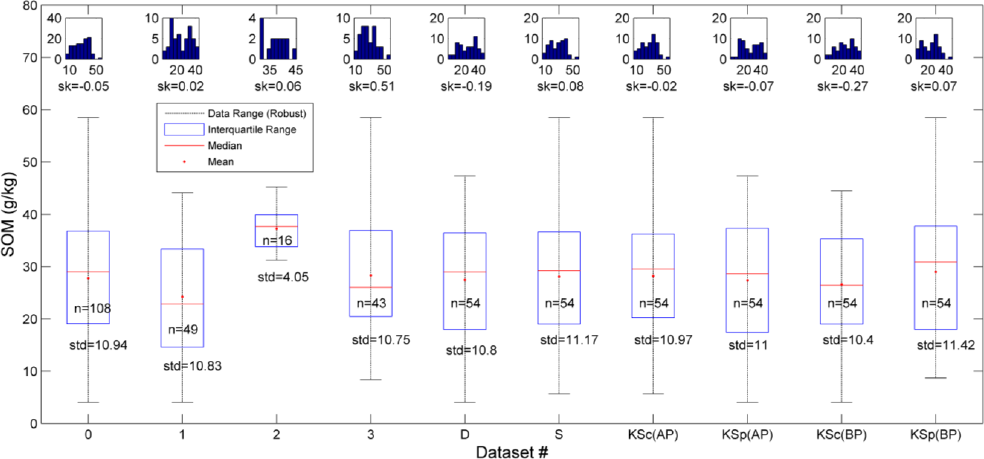
By means of box plots and histograms, Figure 2 presents the statistical characteristics of the SOM content for the total sample set (Dataset 0) and its subsets (divided by location: Dataset 1, Dataset 2 and Dataset 3; divided by the sorting of SOM content: Dataset D and Dataset S; and divided by the Kennard–Stone algorithm: Dataset KSc (AP) and Dataset KSp (AP) for soil samples with pretreatment, Dataset KSc (BP) and Dataset KSp (BP) for soil samples without pretreatment). The SOM contents vary from 4.06 to 58.54 g·kg−1 and show an average of 27.80 g·kg−1 for the 108 samples (Dataset 0). In comparison, the SOM content of the 1381 samples collected in the paddy fields of the Jianghan plain ranged from 9.1 g·kg−1 to 56.5 g·kg−1, with an average of 26.9 g·kg−1 [44].
Dataset 1 and Dataset 3 cover a relatively wide range: 4.06–44.12 g·kg−1 and 8.37–58.54 g·kg−1, showing an average of 24.22 g·kg−1 and 28.35 g·kg−1. Despite the fact that both Dataset 1 and Dataset 2 are from cropland, a narrower range and a much higher mean is observed for Dataset 2: 31.24–45.22 g·kg−1 and 37.30 g·kg−1. With the dividing strategy that attempts to divide the total sample set into two similar subsets, Dataset D and Dataset S have a similar interquartile range, mean and median. The range, standard deviation and skewness of these two datasets, however, are a little different. Such differences could be attributed to the relatively small sample size.
The box plots for these datasets do not suggest any outliers. Histograms indicate the approximate symmetry of the distributions of all the datasets, except for Dataset 3. The skewness of Dataset 3 is 0.51, indicating that the soil samples from this dataset have relatively few high values of SOM content. This could be because Dataset 3 represents soil samples from different land-use types. The histograms of Dataset D and Dataset S only show a little difference, as the skewness of Dataset D < 0 and the skewness of Dataset S > 0. Thus, it is interesting to further examine the performance of models calibrated from datasets with different ranges of SOM content, using other datasets as the prediction datasets.
The Kennard–Stone algorithm was used to select those spectrally-representative samples for model calibrations. For soil samples with pretreatment, the training set, Dataset KSc (AP), has a wider range of SOM content than the test set, Dataset KSp (AP), does. These two datasets are similar in terms of mean, median, standard derivation and skewness. For soil samples without pretreatment, however, the Kennard–Stone divided datasets differ in terms of mean, median, standard derivation and skewness. This could be attributed to the soil moisture and particle size that both affect soil reflectance. Therefore, the Kennard–Stone algorithm does not perform well in the division of soil samples without pretreatment according to their reflectance.
3.2. Correlation Analyses
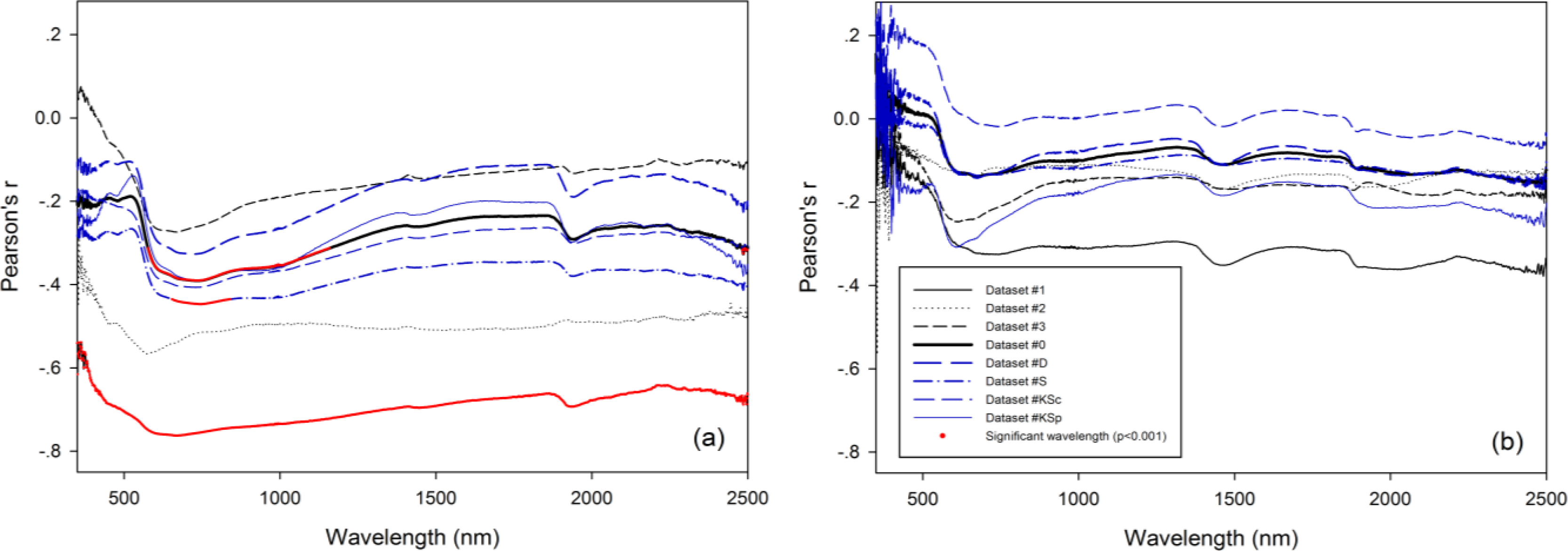
The Pearson correlation between SOM and the reflectance spectra from soil samples with different pretreatments was explored (Figure 3a). For Dataset 1 (samples from the paddy fields), it can be seen that the reflectances of the soil samples with pretreatment are significantly and negatively correlated with the SOM content in the whole spectral region (350–2500 nm) at a confidence interval of 0.001. For the total sample set, the significant wavelengths mainly appear in the region of 550–1200 nm. Dataset D and Dataset S show similar curve shapes to Dataset 0. The curve for Dataset S is generally lower than for Dataset 0, while Dataset D is generally higher. Although the absolute values of Pearson’s r for Dataset S are greater than for Dataset 0 in the region of 550–1200 nm, the significant wavelengths only exist in a narrower region around 750 nm. This result could be attributed to the smaller number of samples in Dataset S, which is half the size of Dataset 0. Dataset KSc and Dataset KSp also show similar curve shapes to Dataset 0. Compared with Dataset D and Dataset S, the correlation coefficient curves for Dataset KSc and Dataset KSp are closer to that of Dataset 0 (Figure 3a). For the soil samples without pretreatment, however, the correlation coefficient curves for Dataset D and Dataset S are closer to that of Dataset 0 (Figure 3b). These results may indicate that the Kennard–Stone algorithm performs better than the “sorted by SOM content” strategy in the division of training and test sets for the soil samples with pretreatment, while the “sorted by SOM content” strategy outperforms the Kennard–Stone algorithm for the soil samples without pretreatment.
No wavelengths are significantly correlated with the SOM content at a confidence interval of 0.001, for Dataset 2, Dataset 3, Dataset D, Dataset KSc and Dataset KSp. It is also observed in Figure 3b that for all eight datasets, no wavelengths (spectra from soil samples without pretreatment) are significantly correlated with the SOM content at a confidence interval of 0.001. This indicates that it is not feasible to estimate the SOM content with a single wavelength.
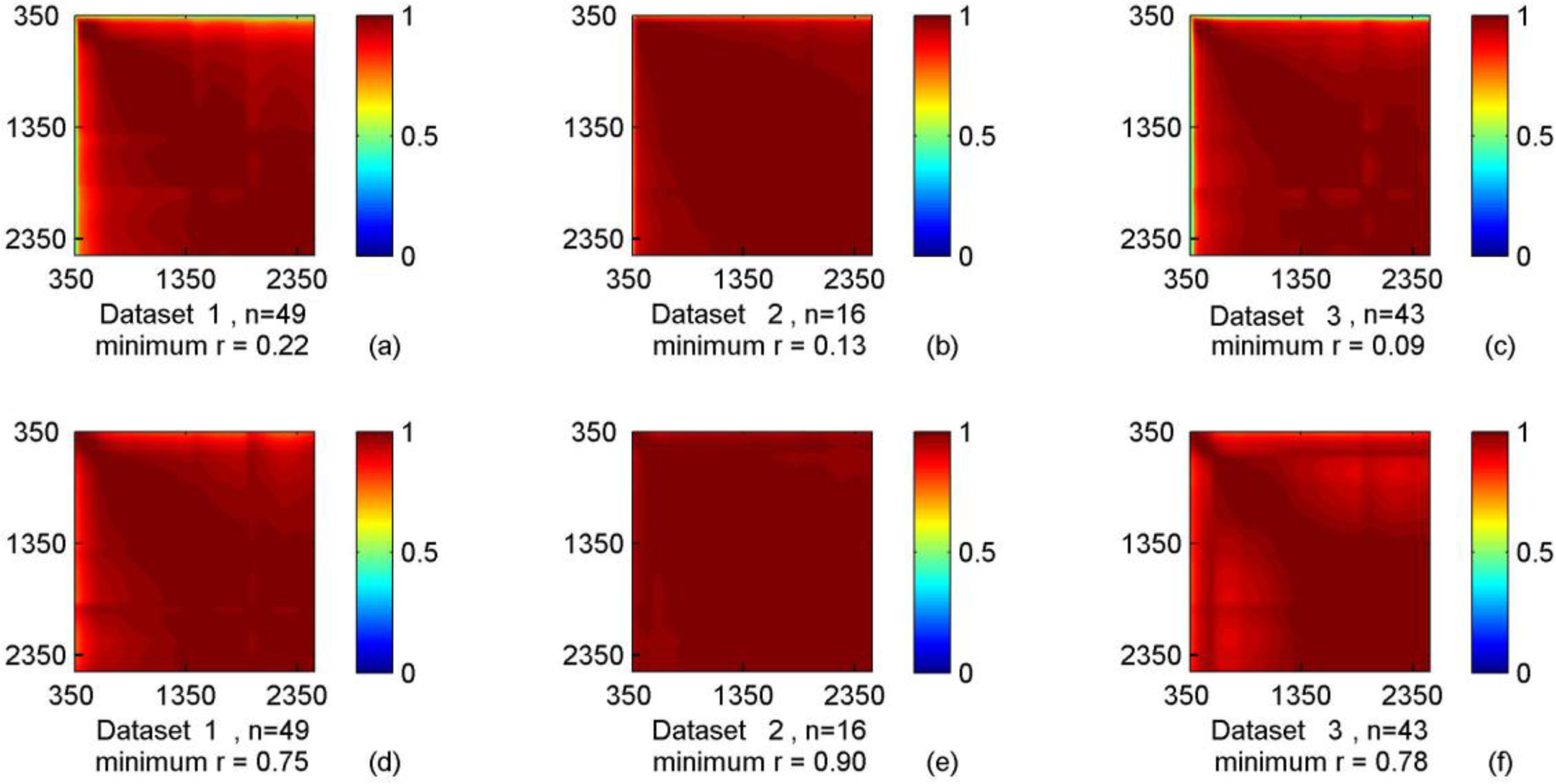
Correlation coefficient maps of the reflectance wavelength pairs from different soil sample sets are shown in Figure 4. The general patterns in the subplots indicate that the spectral wavelengths from the soil samples with different pretreatments are highly correlated with each other in the region of 500–2500 nm (r > 0.8, p < 0.001). With the air-drying, grinding and 2-mm sieving process, the minimum Pearson’s r values between the spectral wavelengths increases from 0.22, 0.13 and 0.09 to 0.75, 0.90 and 0.78 for Dataset 1, Dataset 2, and Dataset 3, respectively. Such significant correlations between spectral variables are known as multicollinearity, which is a typical problem in the VNIR estimation of soil properties. PLSR is a good option to handle such a problem by projecting the highly correlated spectral variables from the original dataset into a small number of latent variables that are orthogonal to each other [38].
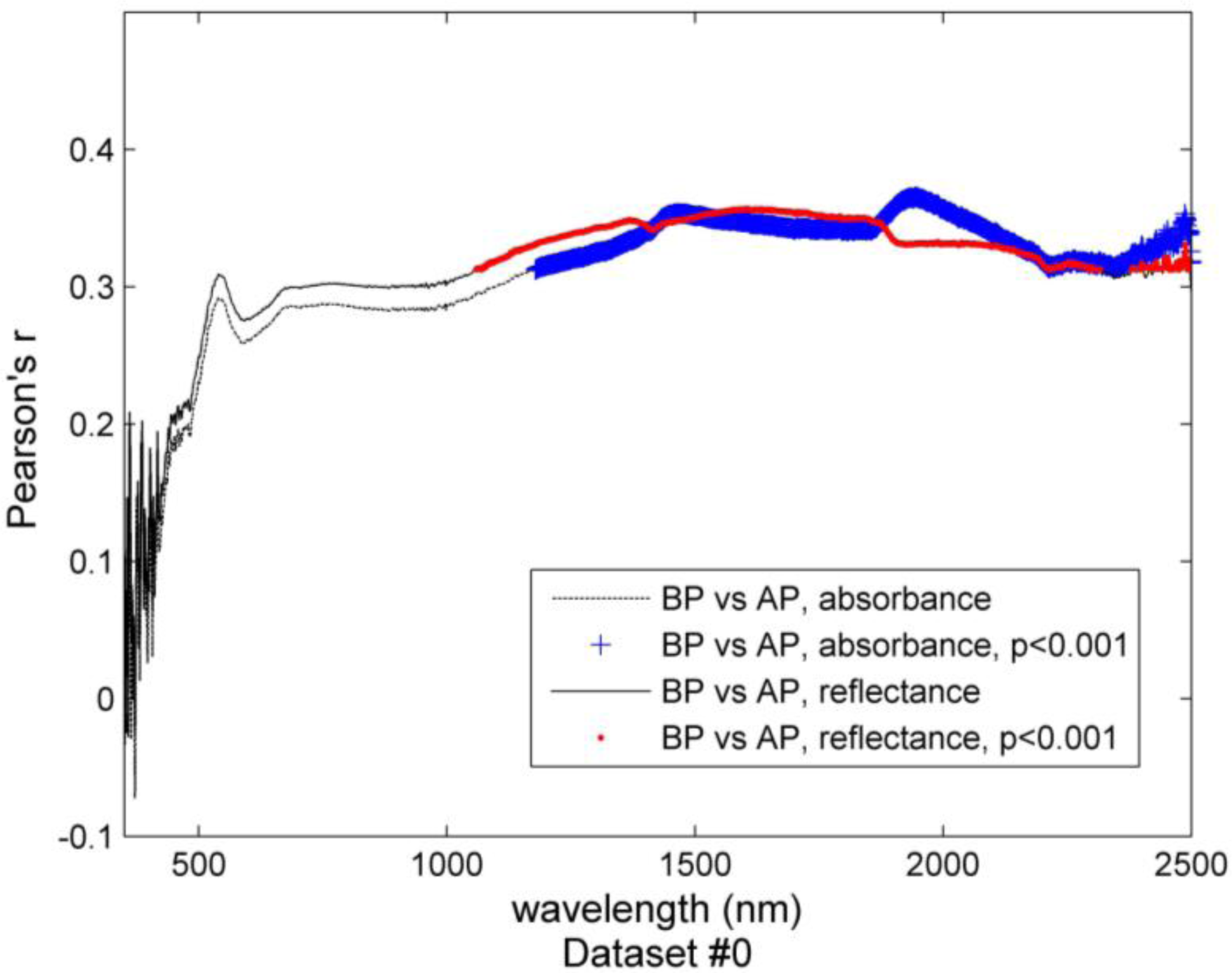
The correlations between spectra at specific wavelengths from soil samples without pretreatments and the spectra at the same wavelength from the pretreated soil samples are explored in Figure 5. The spectral wavelengths that are significantly correlated at a confidence interval of 0.001 are highlighted with specific point symbols. It can be observed that in the visible and short-wave near-infrared region (VSNIR region, 350–1000 nm), the spectral wavelengths from differently prepared soil samples are not significantly correlated (p > 0.001). This indicates that the air-drying, grinding and 2-mm sieving pretreatments significantly modify the linear relationships between the spectral wavelengths in the VSNIR region, but not in most parts of the later region (1000–2500 nm).
3.3. Calibration and Validation
The calibration and validation results of the PLSR models for SOM content estimation are presented in Table 1. For the soil samples without pretreatment, the PLSR models fail to predict the SOM content from the VNIR spectra in all the modeling schemes using both reflectance and absorbance. The r2CV values range from 0.16 to 0.49, while the minimum RMSECV is greater than 7.5 g·kg−1, indicating the failure of the model calibrations. The RPD values in all the schemes are less than 1.4, suggesting that the calibrated models cannot be used for the prediction of SOM content in the specific test set. This could be attributed to the weak signals of SOM in the VNIR region, which are hindered by the moist and/or soil particle effect.
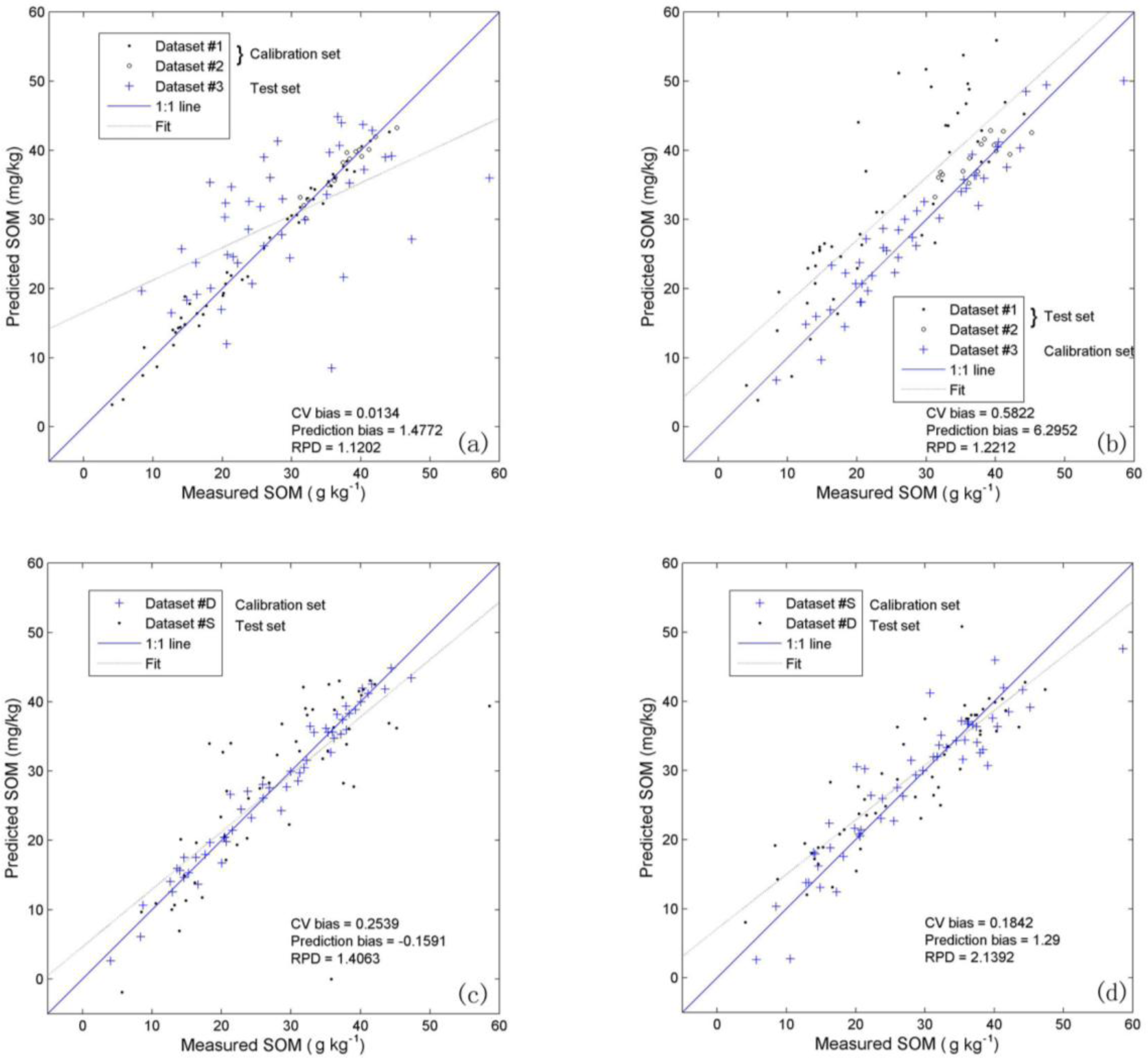
For the soil samples with pretreatment, the models calibrated from Dataset 1 fail to predict the SOM content of Dataset 2 (Scheme 1) or Dataset 3 (Scheme 2) using either reflectance or absorbance. Together with Dataset 1 and Dataset 2 as the training set (Scheme 3), the calibrated models again fail in the prediction of the SOM content of Dataset 3. It is noted that for this scheme, the calibrated models show high values of r2CV (>0.80) and relatively low values of RMSECV. For the reflectance-based model, the CV bias is quite close to zero, indicating the success of the calibrated model from different plots of cropland with different ranges of SOM content (Figure 6a). This indicates that the calibrated models can effectively explain the variance from the calibration dataset. These models, however, do not necessarily perform well in SOM prediction for datasets with different ranges of SOM content, as indicated by the RPD (<1.4) with a relatively low r2Pre and high RMSEP. Such results suggest that a model calibrated from samples collected in cropland cannot be transferred when the soil samples are from different land-use types, as the range of SOM content could be greatly different. Examination of the measured-predicted plot (Figure 6a) of Scheme 3 shows further evidence of the poor transferability of the cropland-based models. The prediction bias is large, with many points of the test set deviating from the 1:1 line.
With regard to Dataset 3 as the training set, the r2CV values reach 0.63 and 0.50 for the reflectance-based and the absorbance-based models, respectively. With Dataset 1 (Scheme 4), Dataset 2 (Scheme 5) or their combination (Scheme 6) as the test set, the coefficients of determination for the test set (r2Pre) range from 0.19 to 0.66 for the absorbance-based models, whereas all the RPD values are less than one. For the reflectance-based models, the r2Pre values are around 0.70, with the RPD ranging from 1.04 to 1.45. Thus, the reflectance-based models generally perform better than the absorbance-based models in these three schemes. It is also noted that the reflectance-based models generally use one more latent variable than the absorbance-based models. The highest RPD value of 1.45 is found with Scheme 5 (Dataset 3 as the training set and Dataset 2 as test set), which indicates a fair model for SOM prediction. It is noted that the mean and median values of Dataset 2 and Dataset 3 are quite different. The SOM content of Dataset 2 is within the range of the SOM content of Dataset 3. This might indicate that the PLSR models calibrated from the reflectance of soil samples, which are from different land-use types, could be operational in the SOM prediction of samples from cropland with a SOM range within that of the training set. This result implicates that a widely applicable SOM prediction model for use in riparian landscapes should be based on a wide range of SOM values and soils from different land-use types. The external validation results of Scheme 6 are shown in Figure 6b. Here, it can be seen that the model-predicted SOM values of Dataset 1 and Dataset 2 are generally greater than the laboratory-measured values. The prediction bias reaches as high as 6.3, and the fit line does not even intersect the 1:1 line in the range of SOM.
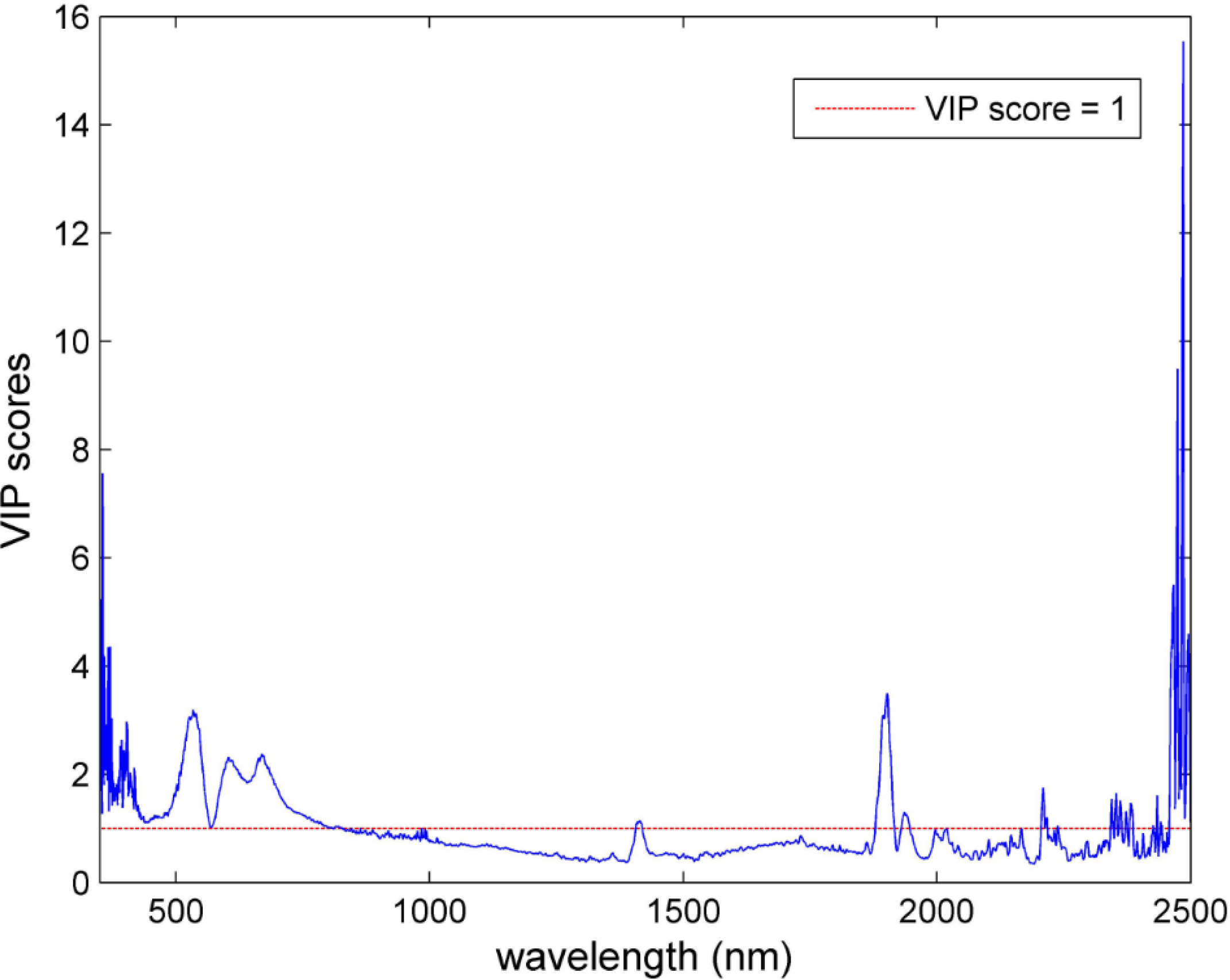
The equal division of Dataset 0 into Dataset D and Dataset S results in two modeling strategies: Dataset D as the calibration set, with Dataset S as the test set (Scheme 7); and Dataset S as the calibration set, with Dataset D as the test set (Scheme 8). The assessment of the two strategies is shown in Table 1. For Scheme 7, the absorbance-based model is superior to the reflectance-based model, with less latent variables and larger r2Pre and RPD values. In the case of Scheme 8, the reflectance-based model performs better in terms of r2Pre, RMSEP and RPD. Comparisons of the reflectance-based models using Scheme 7 and Scheme 8 are shown in Figure 6c,d. The former has a smaller absolute prediction bias and RPD, whereas the latter has an RPD value of greater than 2.0, which indicates a very good result [43]. The VIP scores of this model are shown in Figure 7. The important variables mainly lie in the region of 350–800 nm and around 1900 nm, with some in the region of 2000–2500 nm. This finding reinforces the evidence given by Brown, et al. [45], in which noticeable peaks of VIPs were found at 540 nm, 550 nm and 1910 nm. The comparisons of the statistical distributions of these two datasets indicate that it might be better to use a dataset with a larger range and standard derivation as the calibration set, to ensure a robust model. The results also suggest that models calibrated from a relatively small-sized sample set might be more vulnerable to the variation in the data distribution and, thus, suffer from inconsistent results. Therefore, a larger-sized calibration dataset is suggested for the VNIR estimation of SOM content. Although these two modeling strategies generally outperform the previous schemes, it should be noted that the prior information of SOM content is used in the division of calibration and prediction sets.
Without any prior information about the SOM content, the performance of Scheme 9 is comparable to that of Scheme 7 and Scheme 8. Both RPDs for reflectance-based and absorbance-based models are larger than 1.4 for soil samples with pretreatment. The failure of this scheme in the prediction of SOM content for soil samples without pretreatment may reinforce the previous implication that a widely applicable SOM prediction model should be based on a wide range of SOM contents.
4. Conclusions
In this study, the transferability of several VNIR models for SOM estimation in riparian landscapes has been explored. Three sample division strategies, namely training and test sets divided by sample locations and land-use types, SOM content and the Euclidean distance of soil spectra, have been implemented. Soil samples with and without air-drying, grinding and 2-mm sieving pretreatment were used. Comprehensive comparisons were made for the combinations of different pretreatments for soil samples and modeling strategies.
For the soil samples without pretreatment, the PLSR models failed to predict the SOM content using the VNIR spectra with all the modeling schemes. For the soil samples with pretreatment, models calibrated from the reflectance of a soil sample set with mixed land-use types could be applied in the SOM prediction of cropland soil samples with a suitable range of SOM content (r2Pre = 0.66, RMSE = 2.78 g·kg−1, RPD = 1.45). The models calibrated from cropland soil samples, however, could not be transferred to the SOM prediction of soil samples with diverse land-use types, nor could they be applied in the prediction of SOM content from cropland soil samples in another location in our study, which differed in its distributional characteristic. The correlation analysis revealed that the air-drying, grinding and 2-mm sieving pretreatment significantly modifies the linear relationships between the spectral wavelengths from the soil samples with and without pretreatment in the region of 350–1000 nm. The result also suggests that the wavelengths in the region of 350–1000 nm could be important for SOM estimation in riparian landscapes, considering the failure of the VNIR estimation of SOM content from samples without pretreatment.
The Kennard–Stone algorithm has been regarded as an effective method for the selection of representative subset in the VNIR modeling of soil properties [7,22]. Our studies has revealed that this algorithm performed well in the selection of a representative subset for SOM estimation using the spectra of soil samples with air-drying, grinding and 2-mm sieving pretreatment, but failed in soil samples without this pretreatment. Such results could be important for in situ applications of the soil spectral library in the estimation of SOM content with soil spectra.
Acknowledgments
This research was funded by the National Key Technology R&D Program of China (Grant No. 2012BAH28B02). The authors would like to thank Xuankai Deng and Chengshun Wang for their participation in the fieldwork and Guofeng Wu for his valuable comments.
Author Contributions
Yaolin Liu, Qinghu Jiang and Yiyun Chen designed the research. Qinghu Jiang, Teng Fei and Yiyun Chen performed all the modelling. Junjie Wang, Tiezhu Shi, Kai Guo and Xiran Li participated in the data analyses. Yaolin Liu, Qinghu Jiang and Yiyun Chen were involved in drafting and revising the manuscript.
Conflict of Interest
The authors declare no conflict of interest.
References
- Schmidt, M.W.; Torn, M.S.; Abiven, S.; Dittmar, T.; Guggenberger, G.; Janssens, I.A.; Kleber, M.; Kögel-Knabner, I.; Lehmann, J.; Manning, D.A. Persistence of soil organic matter as an ecosystem property. Nature 2011, 478, 49–56. [Google Scholar]
- Diacono, M.; Castrignanò, A.; Troccoli, A.; de Benedetto, D.; Basso, B.; Rubino, P. Spatial and temporal variability of wheat grain yield and quality in a mediterranean environment: A multivariate geostatistical approach. Field Crops Res 2012, 131, 49–62. [Google Scholar]
- Conforti, M.; Buttafuoco, G.; Leone, A.P.; Aucelli, P.P.C.; Robustelli, G.; Scarciglia, F. Studying the relationship between water-induced soil erosion and soil organic matter using vis–NIR spectroscopy and geomorphological analysis: A case study in southern Italy. Catena 2013, 110, 44–58. [Google Scholar]
- Mander, Ü.; Hayakawa, Y.; Kuusemets, V. Purification processes, ecological functions, planning and design of riparian buffer zones in agricultural watersheds. Ecol. Eng 2005, 24, 421–432. [Google Scholar]
- Zhou, Y.; Wang, Y.; Li, Y.; Zwahlen, F.; Boillat, J. Hydrogeochemical characteristics of central Jianghan Plain, China. Environ. Earth Sci 2013, 68, 765–778. [Google Scholar]
- Zeng, C.; Liu, Y.L.; Liu, Y.F.; Hu, J.M.; Bai, X.G.; Yang, X.Y. An integrated approach for assessing aquatic ecological carrying capacity: A case study of Wujin district in the Tai Lake basin, china. Int. J. Environ. Res. Public Health 2011, 8, 264–280. [Google Scholar]
- Nocita, M.; Stevens, A.; Toth, G.; Panagos, P.; van Wesemael, B.; Montanarella, L. Prediction of soil organic carbon content by diffuse reflectance spectroscopy using a local partial least square regression approach. Soil Biol. Biochem 2014, 68, 337–347. [Google Scholar]
- Conant, R.T.; Ogle, S.M.; Paul, E.A.; Paustian, K. Measuring and monitoring soil organic carbon stocks in agricultural lands for climate mitigation. Front. Ecol. Environ 2010, 9, 169–173. [Google Scholar]
- Bellon-Maurel, V.; Fernandez-Ahumada, E.; Palagos, B.; Roger, J.-M.; McBratney, A. Critical review of chemometric indicators commonly used for assessing the quality of the prediction of soil attributes by NIR spectroscopy. Trends Anal. Chem 2010, 29, 1073–1081. [Google Scholar]
- Ge, Y.; Morgan, C.L.S.; Grunwald, S.; Brown, D.J.; Sarkhot, D.V. Comparison of soil reflectance spectra and calibration models obtained using multiple spectrometers. Geoderma 2011, 161, 202–211. [Google Scholar]
- Gomez, C.; Viscarra Rossel, R.A.; McBratney, A.B. Soil organic carbon prediction by hyperspectral remote sensing and field vis-NIR spectroscopy: An australian case study. Geoderma 2008, 146, 403–411. [Google Scholar]
- Selige, T.; Böhner, J.; Schmidhalter, U. High resolution topsoil mapping using hyperspectral image and field data in multivariate regression modeling procedures. Geoderma 2006, 136, 235–244. [Google Scholar]
- Viscarra Rossel, R.A.; Behrens, T. Using data mining to model and interpret soil diffuse reflectance spectra. Geoderma 2010, 158, 46–54. [Google Scholar]
- Xie, X.-L.; Pan, X.-Z.; Sun, B. Visible and near-infrared diffuse reflectance spectroscopy for prediction of soil properties near a copper smelter. Pedosphere 2012, 22, 351–366. [Google Scholar]
- Ben-Dor, E.; Banin, A. Near-infrared analysis as a rapid method to simultaneously evaluate several soil properties. Soil Sci. Soc. Am. J 1995, 59, 364–372. [Google Scholar]
- Reeves, J., III; McCarty, G. Quantitative analysis of agricultural soils using near infrared reflectance spectroscopy and a fibre-optic probe. J. Near Infrared Spectrosc 2001, 9, 25–34. [Google Scholar]
- Viscarra Rossel, R.A.; Walvoort, D.J.J.; McBratney, A.B.; Janik, L.J.; Skjemstad, J.O. Visible, near infrared, mid infrared or combined diffuse reflectance spectroscopy for simultaneous assessment of various soil properties. Geoderma 2006, 131, 59–75. [Google Scholar]
- Clark, R.N.; King, T.V.V.; Klejwa, M.; Swayze, G.A.; Vergo, N. High spectral resolution reflectance spectroscopy of minerals. J. Geophys. Res 1990, 95, 12653–12680. [Google Scholar]
- Sankey, J.B.; Brown, D.J.; Bernard, M.L.; Lawrence, R.L. Comparing local vs. Global visible and near-infrared (VisNIR) diffuse reflectance spectroscopy (DRS) calibrations for the prediction of soil clay, organic C and inorganic C. Geoderma 2008, 148, 149–158. [Google Scholar]
- Guerrero, C.; Stenberg, B.; Wetterlind, J.; Viscarra Rossel, R.; Maestre, F.; Mouazen, A.; Zornoza, R.; Ruiz-Sinoga, J.; Kuang, B. Assessment of soil organic carbon at local scale with spiked NIR calibrations: Effects of selection and extra-weighting on the spiking subset. Eur. J. Soil Sci 2014, 65, 248–263. [Google Scholar]
- Wetterlind, J.; Stenberg, B. Near-infrared spectroscopy for within-field soil characterization: Small local calibrations compared with national libraries spiked with local samples. Eur. J. Soil Sci 2010, 61, 823–843. [Google Scholar]
- Gogé, F.; Gomez, C.; Jolivet, C.; Joffre, R. Which strategy is best to predict soil properties of a local site from a national vis–NIR database? Geoderma 2014, 213, 1–9. [Google Scholar]
- Guerrero, C.; Zornoza, R.; Gómez, I.; Mataix-Beneyto, J. Spiking of NIR regional models using samples from target sites: Effect of model size on prediction accuracy. Geoderma 2010, 158, 66–77. [Google Scholar]
- Stenberg, B.; Viscarra Rossel, R.A.; Mouazen, A.M.; Wetterlind, J. Visible and Near Infrared Spectroscopy in Soil Science. In Advances in Agronomy; Donald, L.S., Ed.; Academic Press: Waltham, MA, USA, 2010; Volume 107, pp. 163–215. [Google Scholar]
- Stevens, A.; Nocita, M.; Tóth, G.; Montanarella, L.; van Wesemael, B. Prediction of soil organic carbon at the european scale by visible and near infrared reflectance spectroscopy. PLoS One 2013, 8. [Google Scholar] [CrossRef]
- Fang, J.; Rao, S.; Zhao, S. Human-induced long-term changes in the lakes of the Jianghan Plain, Central Yangtze. Front. Ecol. Environ 2005, 3, 186–192. [Google Scholar]
- Wang, H.-Z.; Song, M.-J.; Li, R.-D.; Yu, G.-M. Study on spatial-temporal pattern and driving forces of construction land expansion in Jianghan plain from 1996 to 2005. Resour. Environ. Yangtze Basin 2011, 20, 416–421. [Google Scholar]
- Wang, H.; Shao, Q.; Li, R.; Song, M.; Zhou, Y. Governmental policies drive the LUCC trajectories in the Jianghan Plain. Environ. Monit. Assess 2013, 185, 10521–10536. [Google Scholar]
- Zhao, S.; Fang, J.; Ji, W.; Tang, Z. Lake restoration from impoldering: Impact of land conversion on riparian landscape in Honghu Lake area, Central Yangtze. Agric. Ecosyst. Environ 2003, 95, 111–118. [Google Scholar]
- Stevens, A.; van Wesemael, B.; Bartholomeus, H.; Rosillon, D.; Tychon, B.; Ben-Dor, E. Laboratory, field and airborne spectroscopy for monitoring organic carbon content in agricultural soils. Geoderma 2008, 144, 395–404. [Google Scholar]
- Vohland, M.; Bossung, C.; Frund, H.C. A spectroscopic approach to assess trace-heavy metal contents in contaminated floodplain soils via spectrally active soil components. J. Plant Nutr. Soil Sci 2009, 172, 201–209. [Google Scholar]
- Agricultural Chemistry Committee of China. Conventional Methods of Soil and Agricultural Chemistry Analysis; Science Press: Beijing, China, 1983. (In Chinese) [Google Scholar]
- Rinnan, A.; van den Berg, F.; Engelsen, S.B. Review of the most common pre-processing techniques for near-infrared spectra. TrAC Trend Anal. Chem 2009, 28, 1201–1222. [Google Scholar]
- Bartholomeus, H.M.; Schaepman, M.E.; Kooistra, L.; Stevens, A.; Hoogmoed, W.B.; Spaargaren, O.S.P. Spectral reflectance based indices for soil organic carbon quantification. Geoderma 2008, 145, 28–36. [Google Scholar]
- Cozzolino, D.; Morón, A. Potential of near-infrared reflectance spectroscopy and chemometrics to predict soil organic carbon fractions. Soil Tillage Res 2006, 85, 78–85. [Google Scholar]
- Kennard, R.W.; Stone, L.A. Computer aided design of experiments. Technometrics 1969, 11, 137–148. [Google Scholar]
- Daszykowski, M.; Walczak, B.; Massart, D. Representative subset selection. Anal. Chim. Acta 2002, 468, 91–103. [Google Scholar]
- Wold, S.; Sjöström, M.; Eriksson, L. PLS-regression: A basic tool of chemometrics. Chemom. Intell. Lab. Syst 2001, 58, 109–130. [Google Scholar]
- Viscarra Rossel, R.A. Parles: Software for chemometric analysis of spectroscopic data. Chemom. Intell. Lab. Syst 2008, 90, 72–83. [Google Scholar]
- Wold, S.; Trygg, J.; Berglund, A.; Antti, H. Some recent developments in PLS modeling. Chemom. Intell. Lab. Syst 2001, 58, 131–150. [Google Scholar]
- Chong, I.-G.; Jun, C.-H. Performance of some variable selection methods when multicollinearity is present. Chemom. Intell. Lab. Syst 2005, 78, 103–112. [Google Scholar]
- Chang, C.W.; Laird, D.A. Near-infrared reflectance spectroscopic analysis of soil C and N. Soil Sci 2002, 167, 110–116. [Google Scholar]
- Mouazen, A.M.; Kuang, B.; de Baerdemaeker, J.; Ramon, H. Comparison among principal component, partial least squares and back propagation neural network analyses for accuracy of measurement of selected soil properties with visible and near infrared spectroscopy. Geoderma 2010, 158, 23–31. [Google Scholar]
- Wang, W.; Lu, J.; Lu, M.; Dai, Z.; Li, X. Status quo and variation of soil fertility in paddy field—A case study of Hubei province. Acta Pedol. Sinica 2012, 49, 319–330. (In Chinese). [Google Scholar]
- Brown, D.J.; Shepherd, K.D.; Walsh, M.G.; Mays, M.D.; Reinsch, T.G. Global soil characterization with VNIR diffuse reflectance spectroscopy. Geoderma 2006, 132, 273–290. [Google Scholar]


| Pre-Processing of Spectra | Soil Sample before Pretreatment | Soil Sample after Pretreatment | ||||||||||
|---|---|---|---|---|---|---|---|---|---|---|---|---|
| LVs | r2CV | RMSECV | r2Pre | RMSEP | RPD | LVs | r2CV | RMSECV | r2Pre | RMSEP | RPD | |
| Scheme 1: training set (Dataset 1, N = 49), test set (Dataset 2, N = 16)
| ||||||||||||
| Reflectance | 8 | 0.24 | 10.55 | 0.03 | 8.80 | 0.46 | 8 | 0.84 | 4.39 | 0.18 | 6.16 | 0.66 |
| Absorbance | 2 | 0.16 | 10.00 | 0.08 | 14.28 | 0.28 | 10 | 0.86 | 4.02 | 0.72 | 14.27 | 0.28 |
| Scheme 2: training set (Dataset 1, N = 49), test set (Dataset 3, N = 43)
| ||||||||||||
| Reflectance | 8 | 0.24 | 10.55 | 0.05 | 10.79 | 1.00 | 8 | 0.84 | 4.39 | 0.13 | 16.76 | 0.64 |
| Absorbance | 2 | 0.16 | 10.00 | 0.09 | 11.06 | 0.97 | 10 | 0.86 | 4.02 | 0.09 | 19.42 | 0.55 |
| Scheme 3: training set (Dataset 1 + Dataset 2, N = 65), test set (Dataset 3, N = 43)
| ||||||||||||
| Reflectance | 3 | 0.36 | 8.87 | 0.04 | 17.23 | 0.62 | 13 | 0.89 | 3.74 | 0.30 | 9.59 | 1.12 |
| Absorbance | 3 | 0.38 | 8.78 | 0.09 | 14.67 | 0.73 | 10 | 0.89 | 3.68 | 0.20 | 10.68 | 1.00 |
| Scheme 4: training set (Dataset 3, N = 43), test set (Dataset 1, N = 49)
| ||||||||||||
| Reflectance | 6 | 0.45 | 8.10 | 0.32 | 9.27 | 1.17 | 9 | 0.63 | 6.75 | 0.74 | 10.38 | 1.04 |
| Absorbance | 5 | 0.49 | 7.60 | 0.12 | 10.36 | 1.05 | 8 | 0.50 | 8.05 | 0.64 | 12.8 | 0.85 |
| Scheme 5: training set (Dataset 3, N = 43), test set (Dataset 2, N = 16)
| ||||||||||||
| Reflectance | 6 | 0.45 | 8.10 | 0.24 | 9.60 | 0.42 | 9 | 0.63 | 6.75 | 0.66 | 2.78 | 1.45 |
| Absorbance | 5 | 0.49 | 7.60 | 0.04 | 12.85 | 0.31 | 8 | 0.50 | 8.05 | 0.19 | 4.91 | 0.82 |
| Scheme 6: training set (Dataset 3, N = 43), test set (Dataset 1+ Dataset 2, N = 65)
| ||||||||||||
| Reflectance | 6 | 0.45 | 8.10 | 0.28 | 9.36 | 1.19 | 9 | 0.63 | 6.75 | 0.70 | 9.12 | 1.12 |
| Absorbance | 5 | 0.49 | 7.60 | 0.07 | 11.02 | 1.01 | 8 | 0.50 | 8.05 | 0.46 | 11.38 | 0.98 |
| Scheme 7: training set (Dataset D, N = 54), test set (Dataset S, N = 54)
| ||||||||||||
| Reflectance | 4 | 0.33 | 8.91 | 0.24 | 10.12 | 1.10 | 11 | 0.78 | 5.17 | 0.59 | 7.94 | 1.41 |
| Absorbance | 4 | 0.25 | 9.57 | 0.21 | 10.07 | 1.11 | 8 | 0.65 | 6.60 | 0.62 | 7.05 | 1.58 |
| Scheme 8: training set (Dataset S, N = 54), test set (Dataset D, N = 54)
| ||||||||||||
| Reflectance | 7 | 0.36 | 9.10 | 0.55 | 8.23 | 1.31 | 9 | 0.56 | 7.61 | 0.79 | 5.05 | 2.14 |
| Absorbance | 9 | 0.19 | 11.10 | 0.46 | 8.68 | 1.24 | 9 | 0.50 | 8.37 | 0.65 | 6.61 | 1.63 |
| Scheme 9: training set (Dataset KSc, N = 54), test set (Dataset KSp, N = 54)
| ||||||||||||
| Reflectance | 8 | 0.47 | 7.73 | 0.41 | 9.12 | 1.25 | 7 | 0.52 | 7.72 | 0.70 | 6.11 | 1.80 |
| Absorbance | 7 | 0.18 | 11.00 | 0.36 | 9.04 | 1.21 | 9 | 0.52 | 7.45 | 0.74 | 5.81 | 1.94 |
© 2014 by the authors; licensee MDPI, Basel, Switzerland This article is an open access article distributed under the terms and conditions of the Creative Commons Attribution license (http://creativecommons.org/licenses/by/3.0/).
Share and Cite
Liu, Y.; Jiang, Q.; Fei, T.; Wang, J.; Shi, T.; Guo, K.; Li, X.; Chen, Y. Transferability of a Visible and Near-Infrared Model for Soil Organic Matter Estimation in Riparian Landscapes. Remote Sens. 2014, 6, 4305-4322. https://0-doi-org.brum.beds.ac.uk/10.3390/rs6054305
Liu Y, Jiang Q, Fei T, Wang J, Shi T, Guo K, Li X, Chen Y. Transferability of a Visible and Near-Infrared Model for Soil Organic Matter Estimation in Riparian Landscapes. Remote Sensing. 2014; 6(5):4305-4322. https://0-doi-org.brum.beds.ac.uk/10.3390/rs6054305
Chicago/Turabian StyleLiu, Yaolin, Qinghu Jiang, Teng Fei, Junjie Wang, Tiezhu Shi, Kai Guo, Xiran Li, and Yiyun Chen. 2014. "Transferability of a Visible and Near-Infrared Model for Soil Organic Matter Estimation in Riparian Landscapes" Remote Sensing 6, no. 5: 4305-4322. https://0-doi-org.brum.beds.ac.uk/10.3390/rs6054305