Scattering Mechanisms for the “Ear” Feature of Lop Nur Lake Basin


Abstract
: Lop Nur is a famous dry lake in the arid region of China. It was an important section of the ancient “Silk Road”, famous in history as the prosperous communication channel between Eastern and Western cultures. At present, there is no surface water in Lop Nur Lake basin, and on SAR (Synthetic Aperture Radar) images, it looks like an “Ear”. The objective of this paper is to interpret the Lop Nur phenomenon from the perspective of scattering mechanisms. Based on field investigation and analysis of sample properties, a two-layer scattering structure is proposed with detailed explanations of scattering mechanisms. In view of the rough surface, the MIEM (Modified Integral Equation Model) was introduced to represent air-surface scattering in Lop Nur. Then, a two-layer scattering model was developed which can describe surface scattering contribution. Using polarimetric decomposition, validations were carried out, and the RMSE (root mean square error) values for the HH and VV polarizations were found to be 1.67 dB and 1.06 dB, respectively. Furthermore, according to model parametric analysis, surface roughness was identified as an apparent reason for the “Ear” feature. In addition, the polarimetric decomposition result also showed that the volume scattering part had rich texture information and could portray the “Ear” feature exactly compared with the other two parts. It is maintained that subsurface properties, mainly generating volume scattering, can determine the surface roughness under the certain climate conditions, according to geomorphological dynamics, which can help to develop an inversion technology for Lop Nur.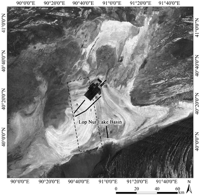
1. Introduction
Lop Nur was a huge lake located at the eastern end of the Tarim Basin, Xinjiang Uygur Autonomous Region, in northwestern China, in an important section of the ancient “Silk Road”, famous in history as the prosperous communication channel between Eastern and Western cultures. At present, Lop Nur has lost its last water drop and appears as an “Ear” feature (interchanging bright-grey appearance) on SAR images (Figure 1); its formation has always been a mystery. Some assumptions have been made about this issue, but they remain to be proven by scientific evidence. Because it is a catchment basin for major rivers in Tarim, Lop Nur is rich in mineral salts, especially potassium deposits. Lop Nur has been described as the “Drought Pole” of the world, with many salts at the surface and very low moisture. With the penetration ability of SAR signals and the arid environment of Lop Nur, it is believed that SAR can detect subsurface targets. To explain the Lop Nur phenomenon more precisely, a proper analysis of scattering mechanisms and an appropriate scattering model are needed, which could help to find reasons for the formation of the “Ear” feature.
In the field of SAR remote sensing technology, analysis of scattering mechanisms and modeling are always the focus. During the last three decades, many experts in electromagnetic calculation have devoted their efforts to developing theoretical scattering models for simple typical targets (Kirchhoff model [1], SPM (Small Perturbation Model) [2], and IEM (Integral Equation Model) [3]). Such models, based on the second Green’s vector theorem, have been used to retrieve target parameters from SAR images. However, under certain circumstances, applying theoretical models like IEM to natural soil surfaces presents inconsistencies compared to experimental measurements. This is why empirical approaches were developed based on field investigations and theoretical analysis [4,5]. In view of application requirements, several researchers have tried to simplify and recombine various theoretical models to establish practical algorithms or models [6]. More recently, numerical simulation methods were used to describe the scattering behavior, which is helpful to analyze the scattering phenomenon and model [7,8]. Therefore, a proper understanding of scattering mechanisms is a prerequisite for using SAR data accurately and is the basis for development of an applicable inversion technology.
SAR is sensitive to the geometric and dielectric properties of its targets. More specifically, as for surface targets, roughness can represent geometric properties, and its contribution to the final backscattering intensity is usually more important than that of dielectric properties. Generally, most algorithms place particular emphasis on excluding the roughness contribution and retrieving parameters related to dielectric properties such as moisture and salinity [9–13]. In scattering models, surface roughness is difficult to describe, and its scattering process or spectral signature is always a focus of study. After the IEM was proposed by Fung in 1992, several researchers tried to modify it to simulate scattering intensity more accurately by means such as multiscale surface roughness spectral functions, transition models for reflection coefficients, and an absolute phase term to describe multiple scattering contributions [14–19]. In the case of rough surfaces or interfaces, the multiple scattering contributions are no longer small and should not be ignored. In the original IEM, the absolute phase term in Green’s function was eliminated to simplify the mathematical manipulations. The absolute phase term represents downward and upward propagating waves, which should contribute, especially in the case of serious roughness, to the total scattered fields. In recent years, based on a scattering modeling of one interface, a two-layer structure composed of two homogeneous media with two interfaces has become a hot topic. Pinel proposed a two-layer scattering model under the geometric optics approximation which describes scattering mechanisms in detail and simulates scattering behavior for some geoscience applications [20,21].
In this research, a scattering structure for Lop Nur has been determined based on field investigations and analysis of physical and chemical properties. Detailed scattering mechanisms have also been described. Two surface scattering processes were emphasized, which occur at surface and subsurface interfaces, respectively. The MIEM (Modified Integral Equation Model) developed by Hsieh in 1996 was introduced to portray the scattering contribution at the air-surface interface. Then, considering scattering at the subsurface interface and the absorption effect during signal propagation in the subsurface layer, a two-layer scattering model was proposed which can represent the surface scattering contribution. Based on analysis of model parameters, an apparent cause of the “Ear” feature has been proposed, and a preliminary discussion of the geomorphological dynamics of surface roughness as controlled by certain subsurface properties, including knowledge of geological evolution in arid regions, has been included.
2. Test Site and Field Investigations
2.1. Test Site Description
Lop Nur is located in the east Tarim Basin in the Xinjiang Uygur Autonomous Region in northwestern China. It is the depocenter of the largest depression basin north of the Tibetan Plateau and the lowest part of the Tarim Basin at the convergence of surface water and groundwater. Historically, major rivers flowed into Lop Nur, including the Tarim, Kongqi, and Qarqan Rivers, carrying tremendous amounts of mineral salts. Due to its special geographical position in the Tarim Basin, mineral salts accumulated and resulted in high salt concentrations in this area, in particular very rich potassium deposits. Lop Nur is the most arid region of Eurasia, with less than 20 mm annual precipitation and over 3000 mm evaporation. It has been called the “Drought Pole” and the “Sea of Death” because of its extremely dry conditions and poor accessibility. A well-developed water system indicates a wet and pleasant environment in the recent history of the Lop Nur region, but today these systems are deteriorating, and rivers have zero flow as a result of the extremely arid climate. The lake area can go through expansion and shrinkage phases several times because of the short-term occurrence of moist airflows or flooding.
2.2. Field Investigation and Sample Collection
A total of five field trips were carried out for this study, with the first field investigation conducted in November 2006. The authors visited the ruins of the Loulan Kingdom and the Lop Nur Lake basin, where lacustrine deposits were sampled along a 41 km profile at intervals of 2 km to the northeast of Lop Nur Lake, as shown in Figure 1. Surface roughness was measured with an instrument made by the authors. One hundred and fifty sticks installed in a frame at intervals of 1 cm were used to record the surface micro-topography, and photographs were taken. The recorded surface pattern was digitized to calculate the RMS (Root Mean Square) height and correlation length. Lacustrine samples from the surface and subsurface were collected at every sampling site, providing a total of 80 samples. Twelve salt crystal and brine samples were also collected from certain sampling sites. The second field investigation was conducted in November 2008, when GPR (Ground Penetrating Radar) was first used to collect Lop Nur subsurface structural information. Three routes, four study areas, and 78 sampling sites were selected along a profile length of 62 km, as shown in Figure 1. These sampling sites were projected onto the georeferenced SAR images. The geographic coordinates of each sampling site were recorded using a GPS (Global Positioning System). Another three field trips were completed in December 2008, April 2010, and November 2010 to determine the northern and western parts of the shoreline and to verify the existence of the shoreline of East Lop Nur Lake, which has been buried by the lacustrine deposits of West Lop Nur Lake.
According to their sedimentary characteristics, six lacustrine deposit samples were collected for each sampling site from the surface to the base of each sampling pit at different depths and numbered as samples one through six. The depth of the pits ranged from 50 cm to 120 cm. The samples were kept fresh in sampling boxes and transported to the laboratory for analysis, including moisture testing, ion content (e.g., Na+, Ca2+, K+, Cl−, SO42−), particle size, pH value, and the real part (ɛ′) and imaginary part (ɛ″) of the dielectric constant.
3. Results and Discussion
3.1. Scattering Mechanisms for Lop Nur Lake Basin
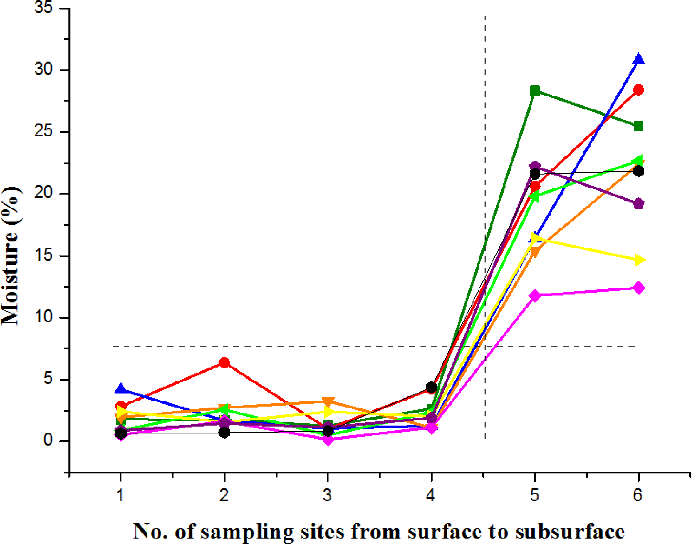
At present, the bed of Lop Nur Lake is extremely flat and uniform, with an endless dry salt crust in all directions. The upper layer of the salt crust is extremely dry with zero water content, resulting in a very low complex dielectric constant (ɛ = 3 − j0.2 for 5.25 GHz, C band, and ɛ = 3.5 − j1 for 1.25 GHz, L band. j means imaginary part of dielectric constant). However, with further digging into the lacustrine deposits, a moist layer was found beneath the upper dry layer on all sampling sites; moreover, at some of the sampling sites, brine was clearly visible and even gushed out. In general, brine is visible at depths of 50–60 cm. Figure 2 shows that the moisture increased abruptly rather than gradually from the fourth sample (average depth of 40 cm) to the fifth sample (average depth of 50 cm) counting from surface to base in each sampling pit. The locations of the fourth and the fifth samples are not fixed, because every sample site has its specific subsurface condition. The average moisture of the first four samples was approximately 2%, but the moisture of the fifth sample increased to 10% at least. From the center to the edge of the lake, the variation of moisture in lacustrine deposits at the same layer position is not obvious.
As for subsurface layers of Lop Nur, the SAR signal cannot penetrate further into the moist layer or into brine water because of the strong electromagnetic attenuation caused by the high dielectric media. The subsurface structure of Lop Nur can be regarded as consisting of two layers with different dielectric properties, an upper dry layer and a moist saline subsurface layer [22]. The GPR detected a boundary between the dry upper layer and the wet lower layer at a depth of approximately 50–55cm ranging from the center to the edge of Lop Nur Lake basin. The microwave penetration path through the dry upper layer of loose aeolian deposits and dry salt crusts of low dielectric constant is shown in Figure 3. Microwaves reached the moist saline layer of lacustrine deposits with very high dielectric constant, which acted as a strong reflector and generated a strong signal back to the SAR antenna. This is why the strong backscattering intensity were obtained in Lop Nur Lake basin, and mean values of HH polarization at L and C band extracted from SAR data were −4 dB and −6 dB, respectively.
From the perspective of scattering mechanisms, the SAR signal can penetrate the rough surface to detect subsurface targets because the top layer has lower dielectric properties, which means that the attenuation effect on the signal is weak. Based on the measured parameters and the analysis described above, a two-layer structure is shown in Figure 4. When the signal arrives at the top interface, strong surface scattering will happen because of the rough micro-topography. Then, the transmission effect will allow a partial signal to propagate sequentially into layer 1, where absorption and volume scattering may attenuate signal intensity. Here, to ease the complexity of modeling and to conduct validation combined with polarimetric decomposition results, only the absorption effect is considered. After attenuation, the signal arrives at the bottom interface, where surface scattering happens once again. Note that in view of the simple sedimentary environment of Lop Nur, the roughness of the bottom interface is not serious. This point agrees with the GPR results, which show that the subsurface interface is much smoother. The signal will transmit continuously into the lower layer, but because of its notable dielectric properties, especially the imaginary part (ɛ″), which accounts for attenuation ability, there is no strong backscattering intensity. In summary, for the scattering mechanisms of Lop Nur, only surface scattering at the top and bottom interfaces and absorption attenuation are considered.
3.2. Scattering Behavior at the Air-Surface Interface
In the Lop Nur Lake basin, the surface micro-topography is rough. The average RMS height (s) is 5.9 cm, and in order to describe scattering behavior at different frequencies, normalized RMS height (ks) is used, k = 2π/λ. Thus, ks for the L-band (1.25 GHz) is 1.54 and for the C-band (5.25 GHz) is 6.6. For such rough surfaces, the original IEM cannot describe scattering behavior exactly. In the late 1980s, surface backscattering enhancement was reported based on both field experiments and numerical simulations. This phenomenon occurs more obviously on rough surfaces. Hsieh developed MIEM, which particularly considers the multiple scattering term [23]. It has been indicated that the multiple scattering contribution appears more important when surface roughness is more pronounced. When multiple scattering becomes notable, backscattering enhancement will occur.
The multiple scattering coefficient consists of two parts, upward and downward contributions. Similarly to the single scattering coefficient, but keeping the absolute phase term in Green’s function with shadowing functions inside and outside the integral for numerical calculation, it can therefore be expressed as:
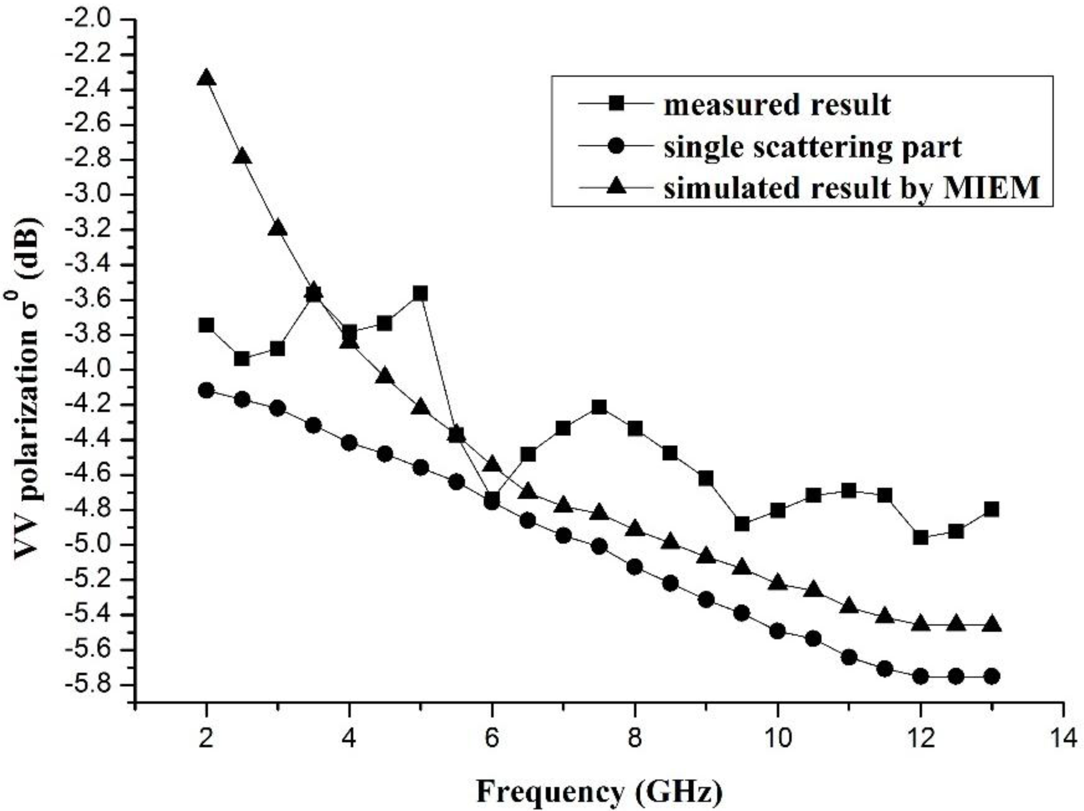
To prove the importance of the multiple scattering part, a standard data set of backscattering coefficients for a rough dielectric surface acquired by EMSL (European Microwave Signature Laboratory) has been used here. This is a Gaussian distributed, Gaussian correlated, and dielectric rough surface. Its RMS height (s) is 2.5 cm, and its correlation length (l) is 6.0 cm. The like- and cross-polarized backscattering measurements were obtained in the frequency range of 2–18 GHz, with incidence angles ranging from 10° to 50°. Figure 5 shows the importance of the multiple scattering part based on MIEM. It has been found that the model including the multiple scattering part can approximate measured data better, especially in the low-frequency band. Actually, the EMSL surface is not extremely rough because its RMS slope under the Gaussian assumption ( ×s/l) is 0.59, which is only a little larger than 0.5. Therefore, the significance of multiple scattering is not clear enough. As for Lop Nur, it is believed that the MIEM can represent scattering behavior at the air-surface interface accurately.
3.3. Surface Scattering for a Two-Layer Structure
Based on field investigations and analysis of the dielectric properties of multiple layers, scattering mechanisms for the Lop Nur Lake basin and their corresponding scattering structures have been identified (Figure 4). Usually, the total scattered intensity from a layered media with irregular boundaries consists of two contributions: one comes from scattering by the top rough interface, and the other from the multiple layers. In mathematical terms,
Actually, all four terms in Equation (2) are often not all important simultaneously. Some approximations can ease the complexity of modeling to make the equation applicable. Generally, the fourth term, Ivgt, is small compared to the other three terms and can be ignored. The volume scattering contribution, Ivt, depends on the propagation path of the signal and the media characteristics. As for the subsurface structure of Lop Nur, the thickness of layer 1 is finite, and generally there is a dielectric interface at depths of 50–55 cm below the surface. In addition, the signal propagation path is also controlled by incidence angle. A small incidence angle can shorten the propagation distance. In extreme situations, vertical incidence means that the effective propagation distance is approximately equal to the thickness of layer 1. Therefore, the finite thickness of layer 1 and the controlled incidence angle can limit the volume scattering contribution, and in this paper, Ivt is not considered. Thus, Equation (2) can be changed as follows to represent the surface scattering of the top surface and bottom interface,
In view of the special surface conditions in Lop Nur, the MIEM is regarded as a specific expression of σ°top. In addition, the bottom interface is much smoother because of the simple sedimentary environment, and the original IEM is used to represent σ°bottom. Considering transmission and absorption effects, the complete expression for σ°bottom is:
To validate the two-layer scattering model, the surface scattering contribution in Lop Nur should be explored first. There is currently much interest in the use of polarimetry for SAR remote sensing. Polarimetric technology can extract physical information from the observed scattering of microwaves by surface and volume structures. The most important observable entity measured by the SAR system is the 3 × 3 coherency matrix [T] or covariance matrix [C]. This matrix accounts for local variations in the scattering matrix and is the lowest operator suitable to extract polarimetric parameters for distributed scattering. Target decomposition theorems are aimed at breaking down the polarimetric scattering signature of a distributed scatter, which is in general given by the superposition of different scattering contributions inside the resolution cell, into a sum of elementary scattering contributions related to specific scattering processes [25]. In this paper, eigenvector-eigenvalue based decomposition, which is based on an eigenvalue analysis of the coherency matrix [26,27], has been used to extract the surface scattering part from SAR images, after which the backscattering coefficients of HH and VV polarization (σ°HH, σ°VV) for this contribution can be calculated.
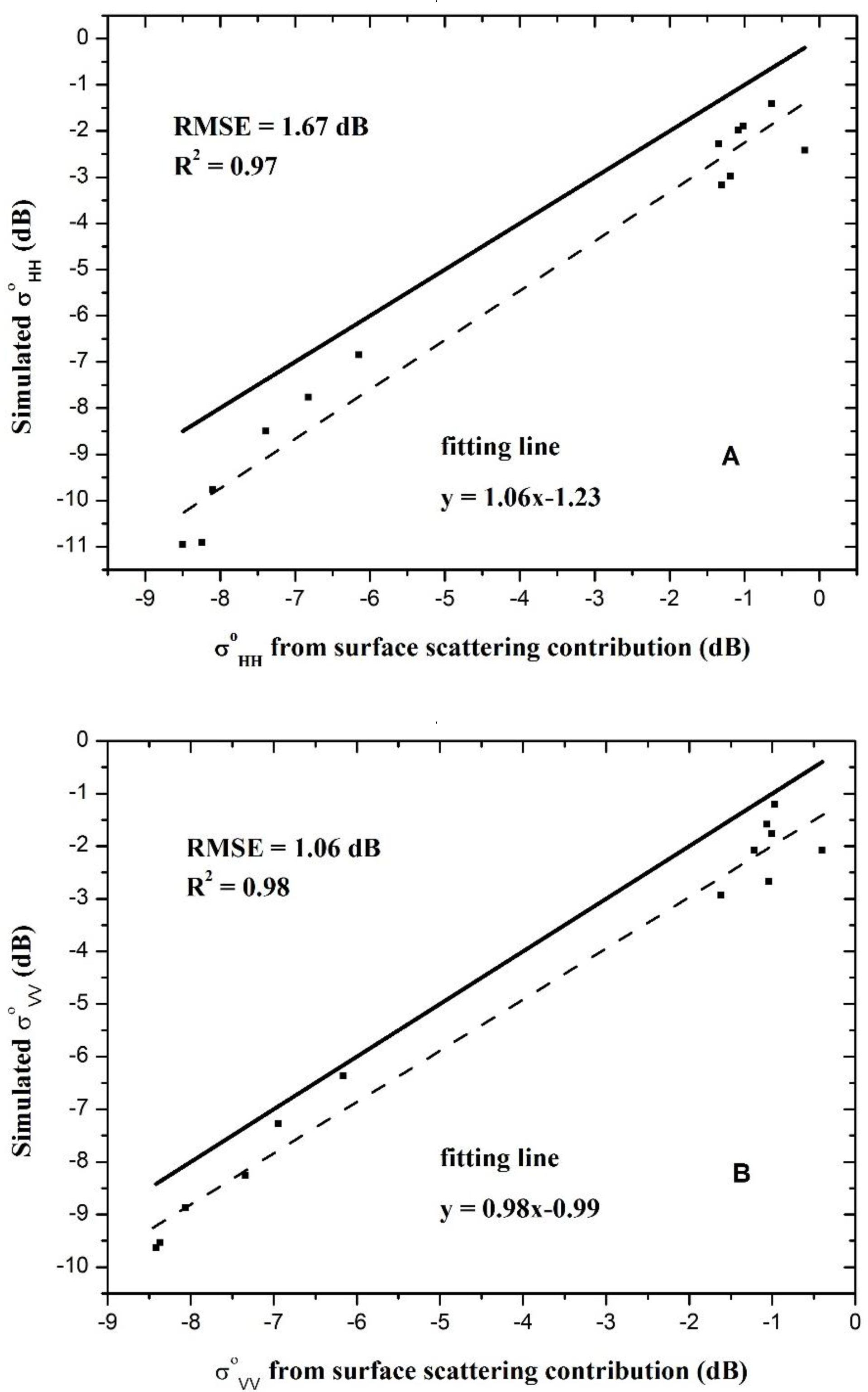
Figure 6 shows a comparison between σ° from the surface scattering contribution using eigenvector-eigenvalue based decomposition and simulated results using the two-layer scattering model. Two scenes of ALOS-PALSAR polarimetric data (L-band, quad-polarization, 23.9° and 25.6° incidence angles for 19 April and 6 May 2009) were used. The input parameters used in these simulations are listed in Table 1. It was found that the two-layer scattering model could represent the surface scattering contribution in Lop Nur, with RMSE values for HH and VV polarization of 1.67 dB and 1.06 dB, respectively. By comparing the solid and dashed lines in each diagram (Figure 6), it is apparent that the simulated results are smaller than the SAR response as a whole. This may be due to a mismatch between the selected window size for polarimetric decomposition and target’s scattering constitution, resulting in confusion of the scattering mechanisms in a resolution cell, or due to the noise level of the SAR system. Nevertheless, the relatively good consistency still shows the applicability of the model.
Among the parameters in the two-layer scattering model, the dielectric properties of layer 1 and the roughness condition of the bottom interface are relatively stable in Lop Nur, and therefore the RMS height at the top surface, the ɛ″ value of layer 2, and the thickness of layer 1 will be considered in parametric analysis. Through 3-D graphic effects, the variation patterns of simulated σ°VV from the two-layer scattering model with RMS height of top surface (s1) and ɛ″ of layer 2 are shown in Figure 7. It has been confirmed that with the increase in s1, the simulated σ°VV values increase drastically. Moreover, different ɛ″ values for layer 2 produce almost the same σ°VV over a large s1 range. Only when s1 is small ɛ″bottom have a relatively deterministic effect on σ°VV. In summary, RMS height of surface should be a major factor in the two-layer scattering model compared with ɛ″ of layer 2. Furthermore, when ɛ” of layer 2 increase, the overall level of simulated σ°VV gets higher, which means the dielectric properties of layer 2 create strong backscattering intensity as a background.
In addition, Figure 8 shows the variation patterns of the simulated σ°VV values with RMS height of top surface and the thickness of layer 1. Although top-layer thickness can influence σ°VV to a certain extent, in Lop Nur it varies over a narrow range, from 30 cm to 70 cm on average (Table 1). In this range, sensitivity to the thickness of layer 1 is limited. However, as for s1, it is still regarded as a strong influencing factor in the model, especially for greater thickness. That means that the RMS height of top surface can largely determine σ°. At this stage, surface roughness is concluded as an apparent reason for the “Ear” feature of Lop Nur.
4. Scattering Contribution to the “Ear” Feature
Through analysis of model parameters, it is evident that the apparent reason for the “Ear” feature of Lop Nur is surface roughness. However, the backscattering intensity in Lop Nur Lake basin is very strong, and a rough surface alone cannot produce the “Ear” feature completely because of its insignificant dielectric properties. With the penetration ability of the SAR signal, it can be seen that the strong backscattering intensity results from subsurface targets with hyper-moist and hyper-saline properties and from surfaces with different roughness conditions lying over these targets, both of which are the causes of the “Ear” feature. Therefore, the “Ear” feature is a joint result of surface roughness conditions and subsurface dielectric properties. However, as for scattering contribution from subsurface, it contains volume scattering in layer 1 and surface scattering at subsurface interface, and the two-layer scattering model as described above only considers the surface scattering part.
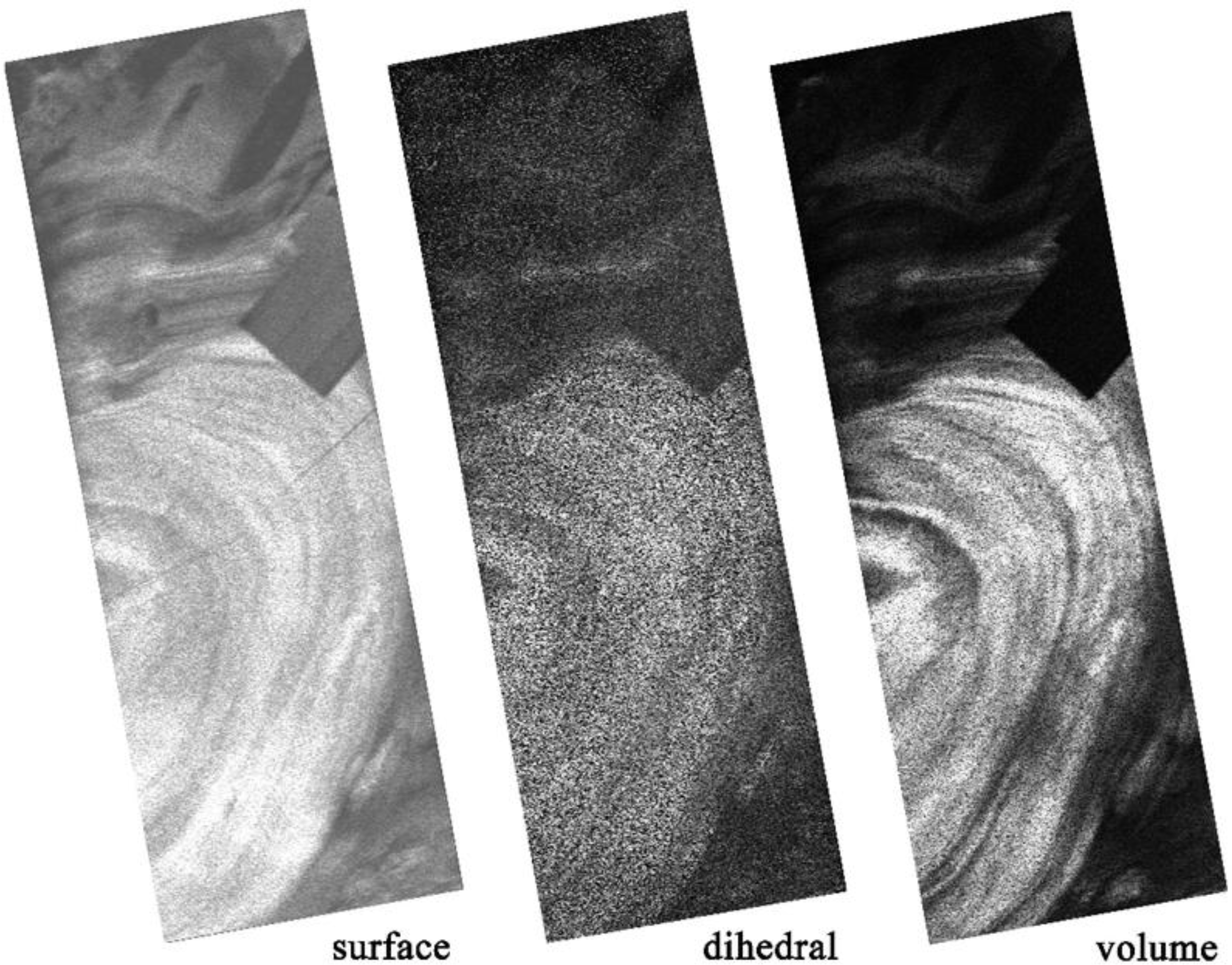
Furthermore, in accordance with scattering mechanisms, to conduct analysis of scattering contributions to the “Ear” feature, model-based decomposition was used to separate the backscattering intensity into several pure scatterings. Such an approach is to use physical models of typical scatters to determine the number and parameterization of each component, and the contribution of each kind of scattering could be obtained [28–32]. Yamaguchi developed a four-component decomposition, which included non-symmetric features to consider more general volume scattering terms, allowing for a relaxation of the azimuthal symmetry assumption to reflection symmetry [33]. Figure 9 shows the Yamaguchi decomposition results in surface scattering, dihedral scattering and volume scattering. The variance of the clarity for the “Ear” feature can be seen from these three images. According to the analysis of scattering mechanism, surface scattering should consist of two parts. One part is generated by the air-surface interface, and the other part arises from subsurface interfaces between media with different dielectric properties. Because of the rough surface conditions of Lop Nur, surface scattering at top surface does not have enough dynamic range to express the differences in SAR response between the bright and grey strips with different image textures. In addition, because of the autochthonous characteristics of Lop Nur, the subsurface interface between media with different dielectric properties is relatively smooth. That means the echo from the subsurface interface cannot exactly represent the image texture. Therefore, the representation of the Lop Nur “Ear” on the surface scattering image was not obvious.
Dihedral scattering occurs mainly at the surface in response to the micro-topography of a target with an approximate dihedral angle structure, and it is able to express the image features to some extent, but not clearly enough. In Lop Nur, salt crusts are distributed in the entire basin, and some of them can form the dihedral structure. However, considering the long-term evolution process and wind erosion, the difference between them is very small, and this is the reason that the dihedral scattering contribution cannot portray the “Ear” feature exactly.
Model-based decomposition reveals that volume scattering is the result of the depolarization effect, which mainly happens in subsurface layers (layer 1). It was determined that this kind of scattering can represent the “Ear” feature exactly, because of its rich texture information compared with the surface scattering part. This result seems inconsistent with the viewpoint stated above that surface roughness is the apparent reason for the “Ear” feature. Actually, the two-layer scattering model ignored the volume scattering part, and just this part has enough dynamic range to show the “Ear” feature. Moreover, the authors maintain that surface patterns and certain subsurface properties are correlated as a result of geomorphological dynamics. Specifically, the bed of Lop Nur Lake was relatively shallow, and no factors other than climate affected its evolution. The brine in the subsurface layers of Lop Nur moved up to the ground surface through capillary rise in saline lacustrine deposits. Higher salinity near the surface with stronger top enrichment and salt crust expansion effects occurred because of the extremely dry weather. Salt crystallization resulted in a very significant change in surface morphology. That means subsurface properties, such as salt content, salt compositions, moisture and so on, can determine the surface roughness under the certain climate conditions. Therefore, it is possible to combine properties from the surface and the subsurface, which is helpful in proposing an inversion technology for Lop Nur using SAR data. Moreover, the content and composition of sedimentary salts are closely related to the paleoclimatic state, which means that reconstruction of the historical evolution of Lop Nur, based on microwave remote sensing technology, remains a future research topic.
5. Conclusions
Based on analysis of the physical and chemical properties of lacustrine deposits, a subsurface scattering structure for Lop Nur has been proposed. The upper layer of the dry mixture of lacustrine deposits with salts and the subsurface layer with high moisture and salinity make significant contributions to a very high intensity on SAR images. SAR has proved to be able to penetrate the superficial dry media and to detect subsurface targets. As a result, detailed scattering mechanisms for the Lop Nur Lake basin have been pointed out. As for scattering behavior at the air-surface interface, MIEM has been introduced to represent its contribution, which particularly refines the impact of multiple scattering. Then, a two-layer scattering model was proposed to describe the surface scattering part. Using polarimetry technology, surface scattering contribution was extracted to validate the developed model. Through 3-D graphic effects, analysis of model parameters was conducted, and the apparent influencing factors on the “Ear” feature of Lop Nur were identified.
Furthermore, the composition of the total backscattering intensity for Lop Nur Lake basin on SAR images has been analyzed. To express the image texture more clearly, model-based decomposition algorithm (Yamaguchi four-component decomposition) was used, and each kind of scattering mechanism was discussed. It was observed that the “Ear” feature of Lop Nur was shown with different degrees of clarity in these three images. It was also confirmed that surface patterns and certain subsurface properties are correlated according to geomorphological dynamics. Based on this viewpoint, it is possible to combine properties from the surface and the subsurface, which is helpful in proposing an inversion technology for Lop Nur using SAR data. In addition, given the paleoclimate significance of the content and composition of sedimentary salts in subsurface layers, reconstruction of the historical evolution of Lop Nur remains a topic for future research.
Acknowledgments
The authors would like to take this opportunity to express their sincere appreciation to the anonymous reviewers. This work was funded by the CAS Knowledge Innovation Program (KZCX2-EW-320), the National Natural Science Foundation of China (41201346, U1303285, 41301394, 41301464), the fund of the State Key Laboratory of Remote Sensing Science (Y1Y00201KZ), IRSA/CAS (Y3SG1900CX, Y1S01200CX), and major special industry application projects (05-Y30B02-9001-13/15-03).
Author Contributions
Huaze Gong was responsible for the development of the two-layer scattering model employed in the research and the corresponding analysis on scattering mechanisms, in addition to reviewing the final manuscript. Yun Shao provided guidance about scattering structure of Lop Nur Lake basin, and some environmental meanings and process were pointed out by her. Tingting Zhang conducted model testing and data analysis, and she also checked the description of this paper in order to make it to be understood better for readers. Long Liu and Zhihong Gao plotted all the figures in this paper and took part in some works of data analysis.
Conflicts of Interest
The authors declare no conflict of interest.
References and Notes
- Ulaby, F.; Moore, R.; Fung, A. Microwave Remote Sensing: Active and Passive. Volume 1-Microwave Remote Sensing Fundamentals and Radiometry; Artech House: Norwood, MA, USA, 1981. [Google Scholar]
- Tsang, L.; Kong, J.A.; Shin, R.T. Theory of Microwave Remote Sensing; Wiley-Interscience: New York, NY, USA, 1985. [Google Scholar]
- Fung, A.K.; Li, Z.; Chen, K. Backscattering from a randomly rough dielectric surface. IEEE Trans. Geosci. Remote Sens 1992, 30, 356–369. [Google Scholar]
- Dubois, P.C.; Van Zyl, J.; Engman, T. Measuring soil moisture with imaging radars. IEEE Trans. Geosci. Remote Sens 1995, 33, 915–926. [Google Scholar]
- Oh, Y.; Sarabandi, K.; Ulaby, F.T. An empirical model and an inversion technique for radar scattering from bare soil surfaces. IEEE Trans. Geosci. Remote Sens 1992, 30, 370–381. [Google Scholar]
- Shi, J.; Wang, J.; Hsu, A.Y.; O’Neill, P.E.; Engman, E.T. Estimation of bare surface soil moisture and surface roughness parameter using L-band SAR image data. IEEE Trans. Geosci. Remote Sens 1997, 35, 1254–1266. [Google Scholar]
- Warnick, K.F.; Chew, W.C. Numerical simulation methods for rough surface scattering. Wave. Random Media 2001, 11, R1–R30. [Google Scholar]
- Simonsen, I. Optics of surface disordered systems: A random walk through rough surface scattering phenomenon. Eur. Phys. J. Spec. Top 2010, 181, 1–103. [Google Scholar]
- Aly, Z.; Bonn, F.J.; Magagi, R. Analysis of the backscattering coefficient of salt-affected soils using modeling and RADARSAT-1 SAR data. IEEE Trans. Geosci. Remote Sens 2007, 45, 332–341. [Google Scholar]
- Metternicht, G. Fuzzy classification of JERS-1 SAR data: an evaluation of its performance for soil salinity mapping. Ecol. Model 1998, 111, 61–74. [Google Scholar]
- Metternicht, G.; Zinck, J. Remote sensing of soil salinity: potentials and constraints. Remote Sens. Environ 2003, 85, 1–20. [Google Scholar]
- Shao, Y.; Hu, Q.; Guo, H.; Lu, Y.; Dong, Q.; Han, C. Effect of dielectric properties of moist salinized soils on backscattering coefficients extracted from RADARSAT image. IEEE Trans. Geosci. Remote Sens 2003, 41, 1879–1888. [Google Scholar]
- Taylor, G.R.; Mah, A.H.; Kruse, F.A.; Kierein-Young, K.S.; Hewson, R.D.; Bennett, B.A. Characterization of saline soils using airborne radar imagery. Remote Sens. Environ 1996, 57, 127–142. [Google Scholar]
- Chen, K.-S.; Wu, T.-D.; Tsay, M.-K.; Fung, A.K. Note on the multiple scattering in an IEM model. IEEE Trans. Geosci. Remote Sens 2000, 38, 249–256. [Google Scholar]
- Fung, A.K.; Chen, K. An update on the IEM surface backscattering model. IEEE Geosci. Remote Sens. Lett 2004, 1, 75–77. [Google Scholar]
- Hsieh, C.-Y.; Fung, A.K.; Nesti, G.; Sieber, A.J.; Coppo, P. A further study of the IEM surface scattering model. IEEE Trans. Geosci. Remote Sens 1997, 35, 901–909. [Google Scholar]
- Manninen, A. Multiscale surface roughness and backscattering-Summary. J. Electromagn. Wave. Appl 1997, 11, 471–475. [Google Scholar]
- Wu, T.-D.; Chen, K.-S. A reappraisal of the validity of the IEM model for backscattering from rough surfaces. IEEE Trans. Geosci. Remote Sens 2004, 42, 743–753. [Google Scholar]
- Wu, T.-D.; Chen, K.-S.; Shi, J.; Fung, A.K. A transition model for the reflection coefficient in surface scattering. IEEE Trans. Geosci. Remote Sens 2001, 39, 2040–2050. [Google Scholar]
- Pinel, N.; Bourlier, C. Scattering from very rough layers under the geometric optics approximation: Further investigation. JOSA A 2008, 25, 1293–1306. [Google Scholar]
- Pinel, N.; Johnson, J.; Bourlier, C. Fully polarimetric scattering from random rough layers under the geometric optics approximation: Geoscience applications. Radio Sci 2011. [Google Scholar] [CrossRef]
- Gong, H.; Shao, Y.; Brisco, B.; Hu, Q.; Tian, W. Modeling the dielectric behavior of saline soil at microwave frequencies. Can. J. Remote Sens 2013, 39, 1–10. [Google Scholar]
- Hsieh, C.Y. Multiple scattering from randomly rough surfaces. Ph.D. Thesis, University of Texas at Arlington, Dallas, USA,. 1996. [Google Scholar]
- Fung, A.K. Microwave Scattering Emission Models and Their Applications; Artech House: Norwood, MA, USA, 1994. [Google Scholar]
- Hajnsek, I.; Pottier, E.; Cloude, S.R. Inversion of surface parameters from polarimetric SAR. IEEE Trans. Geosci. Remote Sens 2003, 41, 727–744. [Google Scholar]
- Cloude, S.R.; Pottier, E. A review of target decomposition theorems in radar polarimetry. IEEE Trans. Geosci. Remote Sens 1996, (34), 498–518. [Google Scholar]
- Cloude, S.R.; Pottier, E. An entropy based classification scheme for land applications of polarimetric SAR. IEEE Trans. Geosci. Remote Sens 1997, 35, 68–78. [Google Scholar]
- Van Zyl, J.J. Unsupervised classification of scattering behavior using radar polarimetry data. IEEE Trans. Geosci. Remote Sens 1989, 27, 36–45. [Google Scholar]
- Freeman, A.; Durden, S.L. A three component model for polarimetric SAR data. IEEE Trans. Geosci. Remote Sens 1998, 36, 963–973. [Google Scholar]
- Yamaguchi, Y.; Moriyama, T.; Ishido, M.; Yamada, H. Four-component scattering model for polarimetric SAR image decomposition. IEEE Trans. Geosci. Remote Sens 2005, 43, 1699–1706. [Google Scholar]
- Yamaguchi, Y.; Sato, A.; Boerner, W.M.; Sato, R.; Yamada, H. Four-component scattering power decomposition with rotation of coherency matrix. IEEE Trans. Geosci. Remote Sens 2011, 49, 2251–2258. [Google Scholar]
- Cui, Y.; Yamaguchi, Y.; Yang, J.; Kobayashi, H.; Park, S.E.; Singh, G. On complete model-based decomposition of polarimetric SAR coherency matrix data. IEEE Trans. Geosci. Remote Sens 2014, 52, 1991–2001. [Google Scholar]
- Cloude, S.R. Polarisation: Applications in Remote Sensing; Oxford University Press: Oxford, UK, 2010. [Google Scholar]


| Serial No. | (s, l)1 * | (ɛ′, ɛ″)1 # | (s, l)2 | (ɛ′, ɛ″)2 | Thickness & |
|---|---|---|---|---|---|
| 1 | (7.00, 50.00) | (4.43, 0.10) | (0.40, 6.10) | (19.94, 71.58) | 35 |
| 2 | (6.49, 45.00) | (3.10, 0.10) | (0.41, 6.00) | (21.48, 67.79) | 36 |
| 3 | (5.38, 38.00) | (3.76, 0.10) | (0.43, 5.90) | (22.18, 63.62) | 30 |
| 4 | (6.12, 40.00) | (3.38, 0.10) | (0.50, 6.70) | (16.35, 33.59) | 40 |
| 5 | (4.81, 30.00) | (3.07, 0.10) | (0.34, 6.60) | (25.10, 77.34) | 32 |
| 6 | (6.18, 46.00) | (5.07, 0.10) | (0.37, 6.10) | (18.41, 49.27) | 60 |
| 7 | (8.36, 56.00) | (3.35, 0.10) | (0.43, 6.30) | (24.50, 92.12) | 47 |
| 8 | (5.80, 52.00) | (3.51, 0.10) | (0.49, 7.30) | (33.30, 112.41) | 55 |
| 9 | (5.16, 47.00) | (3.35, 0.10) | (0.36, 6.60) | (12.05, 32.08) | 70 |
| 10 | (3.83, 35.00) | (3.36, 0.10) | (0.45, 6.56) | (27.31, 80.67) | 55 |
| 11 | (6.89, 85.00) | (3.63, 0.10) | (0.38, 6.80) | (25.47, 75.61) | 48 |
| 12 | (3.91, 50.00) | (4.28, 0.10) | (0.55, 6.30) | (22.29, 61.54) | 56 |
| 13 | (4.89, 50.00) | (3.64, 0.10) | (0.68, 6.40) | (27.69, 85.62) | 55 |
*Subscripts 1 and 2 are for layer 1 and layer 2, respectively (Figure 4). Roughness condition is represented by RMS height (s) and correlation length (l), and they are shown in centimeter. The interface between layer 1 and layer 2 is measured by GPR and field surveys.#The ɛ′ and ɛ″ are the real and imaginary parts of dielectric constant.&Thickness value means the thickness of layer 1, shown in centimeter.
© 2014 by the authors; licensee MDPI, Basel, Switzerland This article is an open access article distributed under the terms and conditions of the Creative Commons Attribution license (http://creativecommons.org/licenses/by/3.0/).
Share and Cite
Gong, H.; Shao, Y.; Zhang, T.; Liu, L.; Gao, Z. Scattering Mechanisms for the “Ear” Feature of Lop Nur Lake Basin. Remote Sens. 2014, 6, 4546-4562. https://0-doi-org.brum.beds.ac.uk/10.3390/rs6054546
Gong H, Shao Y, Zhang T, Liu L, Gao Z. Scattering Mechanisms for the “Ear” Feature of Lop Nur Lake Basin. Remote Sensing. 2014; 6(5):4546-4562. https://0-doi-org.brum.beds.ac.uk/10.3390/rs6054546
Chicago/Turabian StyleGong, Huaze, Yun Shao, Tingting Zhang, Long Liu, and Zhihong Gao. 2014. "Scattering Mechanisms for the “Ear” Feature of Lop Nur Lake Basin" Remote Sensing 6, no. 5: 4546-4562. https://0-doi-org.brum.beds.ac.uk/10.3390/rs6054546