Carbon Stock Assessment Using Remote Sensing and Forest Inventory Data in Savannakhet, Lao PDR

Abstract
:1. Introduction
2. Methods
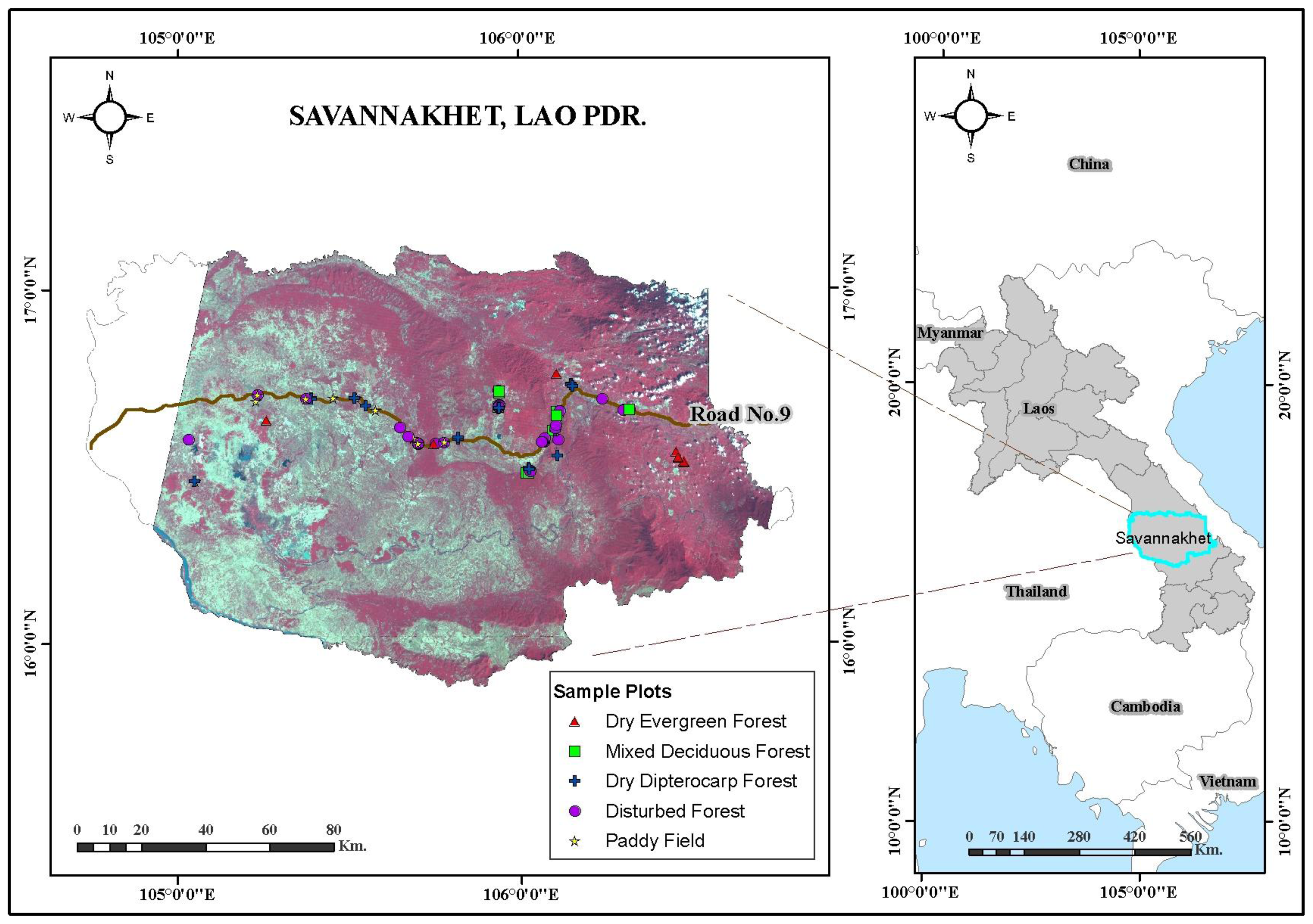
2.1. Study Area
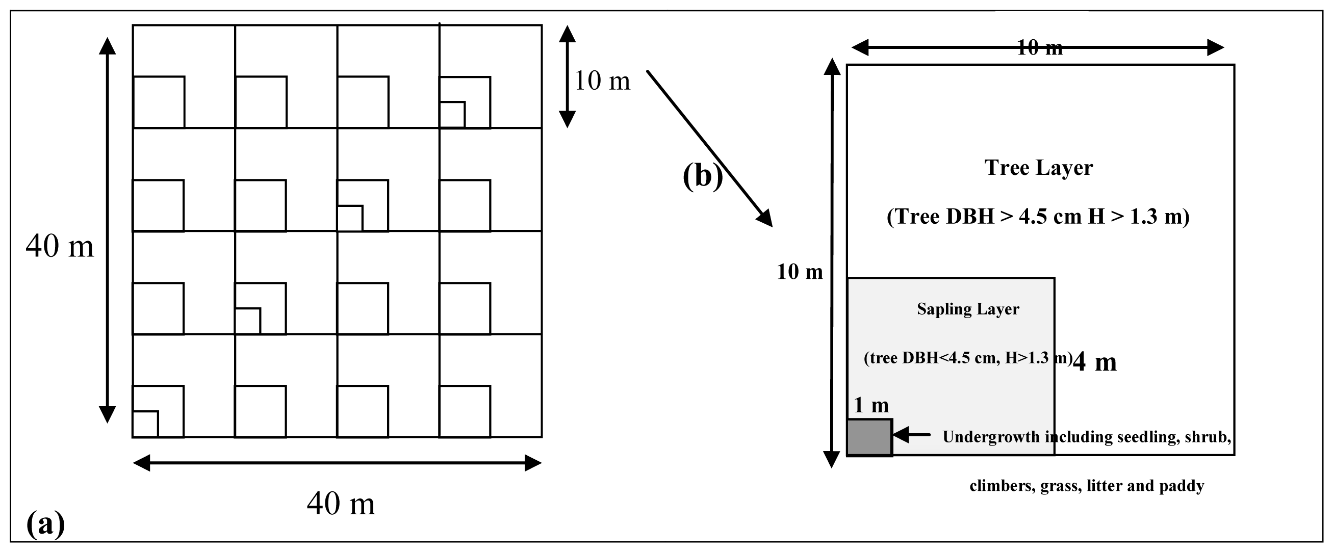
2.2. Field Data Collection
2.3. AGB and Soil Carbon Analysis from Field Data
2.4. Land-Cover Classification Method
2.5. The Correlation between AGB and RS Data
- Raw Landsat bands (B1–B5 and B7) as reflectance;
- VIs, including the simple ratio (SR), difference vegetation index (DVI), normalized difference vegetation index (NDVI), ratio vegetation index (RVI), global environmental monitoring index (GEMI), soil-adjusted vegetation index (SAVI), enhanced vegetation index (EVI), tasseled cap index of greenness (TCG), tasseled cap index of brightness (TCB), and tasseled cap index of wetness (TCW); and
- Topographically derived variables at a spatial resolution of 90 m, including elevation data generated from the SRTM 90-m digital elevation model (DEM) downloaded from the USGS.
2.6. Model Validation
3. Results and Discussion
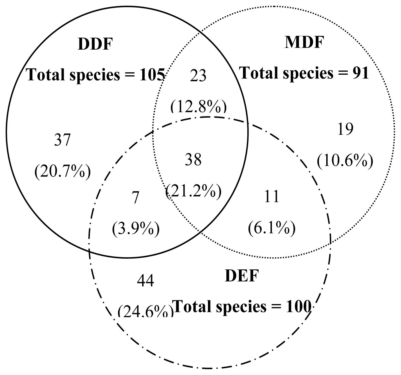
3.1. Vegetation Structure and Forest Composition
3.2. AGB and Soil Carbon Analysis from Field Data
3.2.1. The AGB Analysis of Each Component from Field Data
3.2.2. Total AGB Analysis of Land-Cover Types from Field Data
3.2.3. Soil Carbon Analysis from Field Data
3.2.4. Carbon Stock Analysis from Field Data
3.3. RS-Based Biomass Model
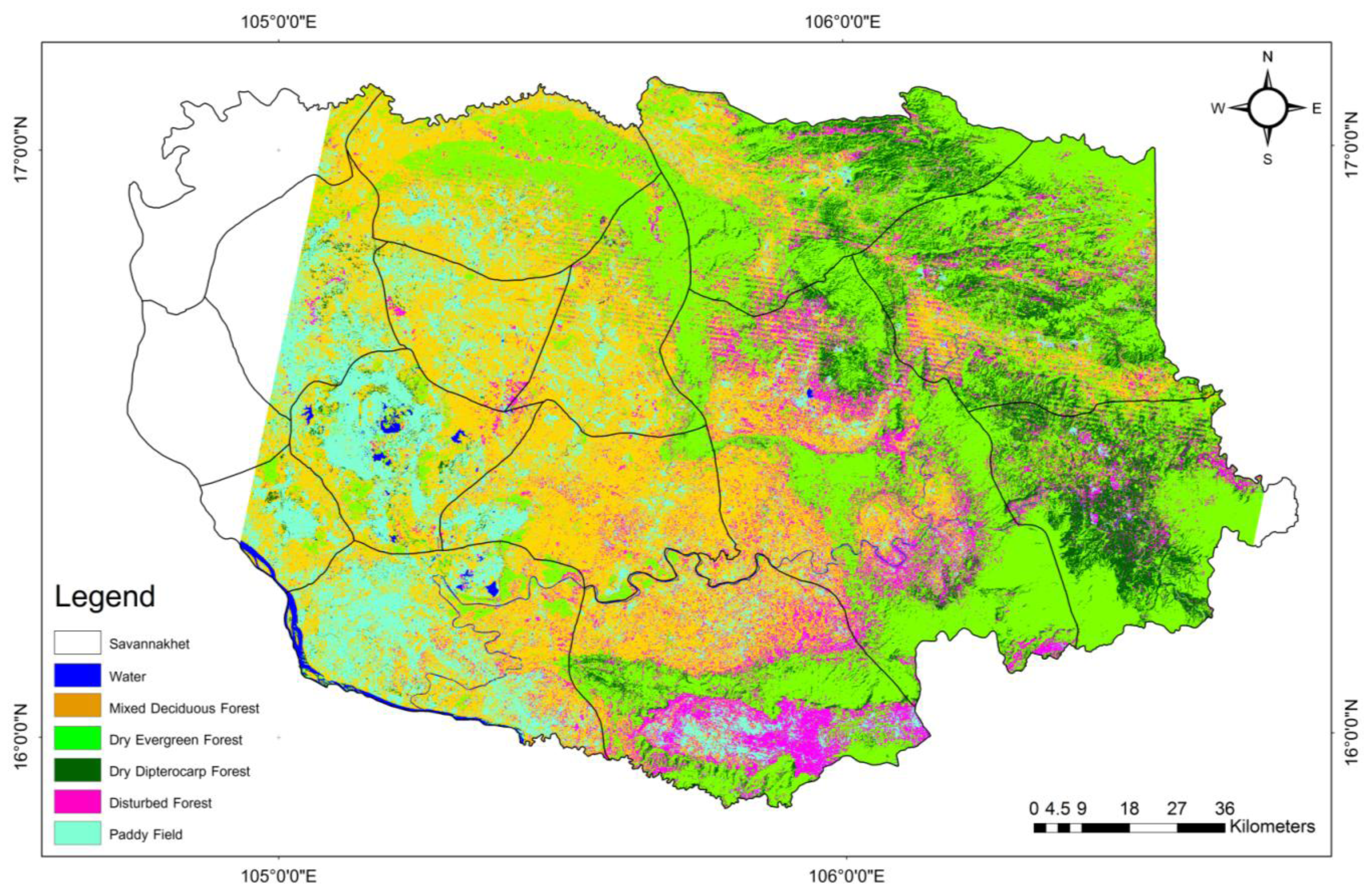
3.3.1. Land-Cover Classification
3.3.2. The AGB Regression Model
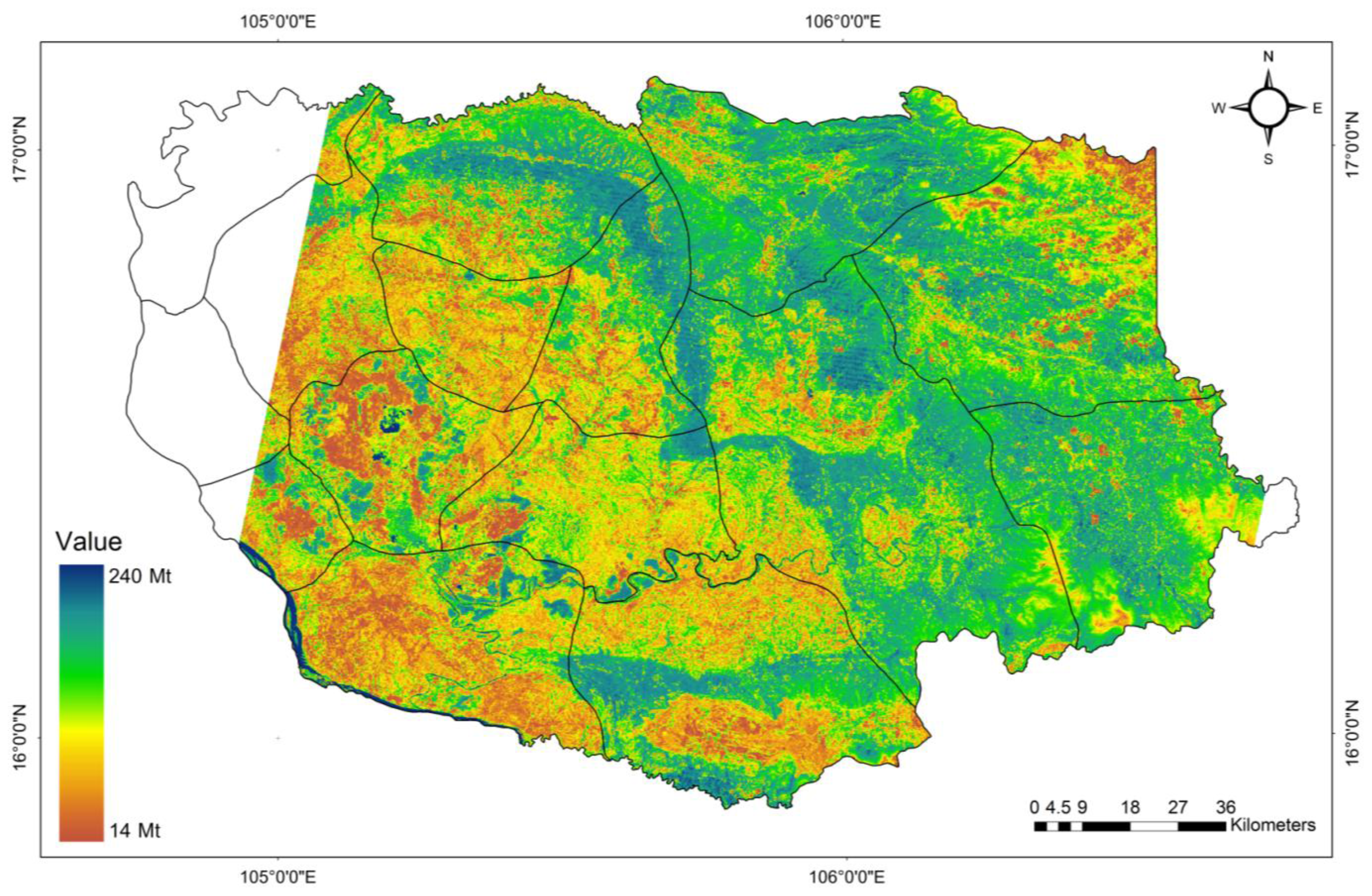
3.3.3. Total Carbon Stock in the Study Area
4. Conclusions
Acknowledgments
Appendix

| Land Cover | Independent | Variable | Constant | Coefficient | R | p-Value |
|---|---|---|---|---|---|---|
| DEF | TM Bands | TM1 | 123.855 | −1.255 | 0.366 | 0.268 |
| TM2 | 200.799 | −5.033 | 0.329 | 0.323 | ||
| TM3 | 164.703 | −5.016 | 0.31 | 0.354 | ||
| TM4 | 49.622 | 0.185 | 0.144 | 0.673 | ||
| TM5 | 212.605 | −1.941 | 0.424 | 0.194 | ||
| TM7 | 325.911 | −10.816 | 0.721 | 0.012 | ||
| VIs | SR | 41.63 | 5.311 | 0.23 | 0.497 | |
| DVI | 52.466 | 0.197 | 0.161 | 0.637 | ||
| NDVI | 44.322 | 36.591 | 0.203 | 0.549 | ||
| RVI | 74.483 | −30.21 | 0.185 | 0.585 | ||
| GEMI | 59.449 | 0.001 | 0.104 | 0.762 | ||
| SAVI | 44.346 | 24.476 | 0.203 | 0.549 | ||
| EVI | 53.628 | −3.323 | 0.198 | 0.559 | ||
| TCG | 55.742 | 0.289 | 0.192 | 0.571 | ||
| TCB | 101.013 | −0.288 | 0.109 | 0.751 | ||
| TCW | 90.012 | 1.48 | 0.383 | 0.244 | ||
| Topographic | Elevation | 18.086 | 0.145 | 0.312 | 0.351 | |
| MDF | TM Bands | TM1 | −45.634 | 3.203 | 0.163 | 0.654 |
| TM2 | 103.076 | 1.599 | 0.031 | 0.931 | ||
| TM3 | 84.647 | 2.586 | 0.117 | 0.748 | ||
| TM4 | −7.797 | 2.92 | 0.504 | 0.137 | ||
| TM5 | 402.993 | −3.102 | 0.198 | 0.584 | ||
| TM7 | 160.067 | −0.359 | 0.018 | 0.96 | ||
| VIs | SR | −131.759 | 138.281 | 0.69 | 0.027 | |
| DVI | 29.349 | 4.193 | 0.586 | 0.075 | ||
| NDVI | −23.569 | 590.49 | 0.65 | 0.055 | ||
| RVI | 414.139 | −458.119 | 0.622 | 0.056 | ||
| GEMI | 57.203 | 0.068 | 0.581 | 0.078 | ||
| SAVI | −23.013 | 394.673 | 0.694 | 0.042 | ||
| EVI | 39.471 | −358.781 | 0.544 | 0.104 | ||
| TCG | 132.285 | 6.638 | 0.614 | 0.059 | ||
| TCB | −71.973 | 1.92 | 0.301 | 0.398 | ||
| TCW | 403.099 | 8.689 | 0.605 | 0.064 | ||
| Topographic | Elevation | 242.599 | −0.385 | 0.122 | 0.736 | |
| DDF | TM Bands | TM1 | 11.748 | 0.613 | 0.265 | 0.273 |
| TM2 | 110.203 | −2.111 | 0.297 | 0.217 | ||
| TM3 | 81.724 | −1.361 | 0.292 | 0.225 | ||
| TM4 | 101.633 | −0.796 | 0.737 | 0.0003 | ||
| TM5 | 50.954 | −0.045 | 0.021 | 0.931 | ||
| TM7 | 46.938 | 0.02 | 0.005 | 0.984 | ||
| VIs | SR | 82.694 | −12.828 | 0.536 | 0.018 | |
| DVI | 83.058 | −0.829 | 0.717 | 0.001 | ||
| NDVI | 101.001 | −121.166 | 0.634 | 0.004 | ||
| RVI | −3.662 | 129.432 | 0.697 | 0.001 | ||
| GEMI | 65.501 | −0.008 | 0.666 | 0.002 | ||
| SAVI | 100.901 | −81.064 | 0.594 | 0.007 | ||
| EVI | 61.109 | 19.455 | 0.566 | 0.011 | ||
| TCG | 60.642 | −0.966 | 0.684 | 0.001 | ||
| TCB | 143.592 | −0.798 | 0.56 | 0.013 | ||
| TCW | 23.501 | −1.126 | 0.517 | 0.023 | ||
| Topographic | Elevation | −82.038 | 0.645 | 0.439 | 0.06 | |
| DF | TM Bands | TM1 | −10.123 | 0.644 | 0.234 | 0.221 |
| TM2 | 31.381 | −0.081 | 0.015 | 0.937 | ||
| TM3 | 34.893 | −0.237 | 0.055 | 0.778 | ||
| TM4 | 96.32 | −0.846 | 0.445 | 0.015 | ||
| TM5 | 40.879 | −0.135 | 0.104 | 0.591 | ||
| TM7 | 32.519 | −0.115 | 0.053 | 0.784 | ||
| VIs | SR | 57.476 | −8.613 | 0.314 | 0.097 | |
| DVI | 68.09 | −0.724 | 0.401 | 0.031 | ||
| NDVI | 67.291 | −75.413 | 0.298 | 0.116 | ||
| RVI | 1.097 | 83.44 | 0.37 | 0.048 | ||
| GEMI | 47.979 | −0.006 | 0.373 | 0.046 | ||
| SAVI | 67.388 | −50.646 | 0.271 | 0.155 | ||
| EVI | 44.601 | 19.81 | 0.402 | 0.031 | ||
| TCG | 46.782 | −0.868 | 0.405 | 0.029 | ||
| TCB | 70.735 | −0.31 | 0.221 | 0.25 | ||
| TCW | 28.632 | −0.008 | 0.005 | 0.979 | ||
| Topographic | Elevation | −87.027 | 0.574 | 0.412 | 0.026 | |
| PFi | TM Bands | TM1 | −21.89 | 0.562 | 0.303 | 0.365 |
| TM2 | 38.16 | −0.762 | 0.154 | 0.652 | ||
| TM3 | 29.51 | −0.556 | 0.206 | 0.544 | ||
| TM4 | 60.606 | −0.609 | 0.647 | 0.031 | ||
| TM5 | 28.145 | −0.174 | 0.115 | 0.731 | ||
| TM7 | 27.007 | −0.444 | 0.207 | 0.541 | ||
| VIs | SR | 34.562 | −8.333 | 0.433 | 0.184 | |
| DVI | 41.743 | −0.608 | 0.609 | 0.047 | ||
| NDVI | 51.703 | −93.096 | 0.612 | 0.045 | ||
| RVI | −30.766 | 103.482 | 0.616 | 0.043 | ||
| GEMI | 25.165 | −0.005 | 0.464 | 0.15 | ||
| SAVI | 51.63 | −62.232 | 0.426 | 0.191 | ||
| EVI | 23.573 | 12.683 | 0.43 | 0.187 | ||
| TCG | 23.94 | −0.695 | 0.58 | 0.061 | ||
| TCB | 72.31 | −0.431 | 0.434 | 0.182 | ||
| TCW | −1.596 | −0.524 | 0.271 | 0.42 | ||
| Topographic | Elevation | −125.23 | 0.75 | 0.506 | 0.112 |
Conflicts of Interest
- Author ContributionsPhutchard Vicharnakorn, Rajendra P. Shrestha, Masahiko Nagai, Abdul P. Salam, and Somboon Kiratiprayoon developed the research concept and methods. Phutchard Vicharnakorn and the GMS-EOC teams collected and prepared the data. Phutchard Vicharnakorn conducted the research. Phutchard Vicharnakorn and Prasong Thammapala performed and interpreted the data analyses, which were then discussed with all of the authors. Phutchard Vicharnakorn wrote the manuscript with contributions from all of the authors.
References
- Food and Agriculture Organization of the United Nations (FAO), State of World’s Forest; Food FAO: Rome, Italy, 2011.
- Gullison, R.E.; Frumhoff, P.C.; Canadell, J.G.; Field, C.B.; Nepstad, D.C.; Hayhoe, K.; Avissar, R.; Curran, L.M.; Friedlingstein, P.; Jones, C.D.; et al. Tropical forests and climate policy. Science 2007, 316, 985–986. [Google Scholar]
- Intergovernmental Panel on Climate Change (IPCC), Climate Change 2007: The Physical Science Basis: Working Group I Contribution to the Fourth Assessment Report of the IPCC; Cambridge University Press: Cambridge, UK, 2007.
- Brown, S. Estimating Biomass and Biomass Change of Tropical Forests; FAO Forest Resources Assessment Publication: Roma, Italy, 1997; p. 55. [Google Scholar]
- Achard, F.; Eva, H.D.; Stibig, H.; Mayaux, P.; Gallego, J.; Richards, T.; Malingreau, J. Determination of deforestation rates of the World’s humid tropical forests. Science 2002, 297, 999–1002. [Google Scholar]
- Mokany, K.; Raison, J.R.; Prokushkin, A.S. Critical analysis of root-shoot rations in terrestrial biomes. Glob. Chang. Biol 2006, 12, 84–96. [Google Scholar]
- Houghton, R.A.; Hall, F.; Goetz, S. Importance of biomass in the global carbon cycle. J. Geophys. Res 2009, 114, 1–13. [Google Scholar]
- International Conference on Emergency Medicine (ICEM), Lao PDR National Report on Protected Areas and Development. In Review of Protected Areas and Development in the Lower Mekong River Region; ICEM: Indooroopilly, QLD, Australia, 2003; p. 101.
- Attarchi, S.; Gloaguen, R. Improving of above groud biomass using dual polarimetric PALSAR and ETM+ data in the Hyrcanian fore tainnuomts (Iran). Remote Sens 2014, 6, 3693–3715. [Google Scholar]
- Maynard, C.L.; Lawrence, R.L.; Nielsen, G.A.; Decker, G. Modeling vegetation amount using bandwise regression and ecological site descriptions as an alternative to vegetation indices. GISci. Remote Sens 2007, 44, 68–81. [Google Scholar]
- Main-Knorn, M.; Moisen, G.G.; Healey, S.P.; Keeton, W.S.; Freeman, E.A.; Hostert, P. Evaluating the remote sensing and inventory-based estimation of biomass in the Western Carpathians. Remote Sens 2011, 3, 1427–1446. [Google Scholar]
- Neigh, C.S.R.; Bolton, D.K.; Diabate, M.; Williams, J.J.; Carvalhais, N. An automated approach to map the history of forest disturbance from insect mortality and harvest with Landsat Time-Series data. Remote Sens 2014, 6, 2782–2808. [Google Scholar]
- Lu, D. The potential and challenge of remote sensing-based biomass estimation. Int. J. Remote Sens 2006, 27, 1297–1328. [Google Scholar]
- Ramankutty, N.; Gibbs, H.K.; Achard, F.; DeFries, R.; Foley, J.A.; Houghton, R.A. Challenges to estimating carbon emissions from tropical deforestation. Glob. Chang. Biol 2007, 13, 51–66. [Google Scholar]
- Somphone, C. Participatory Forest Management: A Research Study in Savannakhet Province, Laos. In Laos Country Report 2003; Institute for Global Environmental Strategies: Kanagawa, Japan, 2004; pp. 44–45. [Google Scholar]
- Kankare, V.; Vastaranta, M.; Holopainen, M.; Raty, M.; Yu, X.; Hyyppa, J.; Hyyppa, H.; Alho, P.; Viitala, R. Retrieval of forest aboveground biomass and stem volume with airborne scanning LiDAR. Remote Sens 2013, 5, 2257–2274. [Google Scholar]
- Wannasiri, W.; Masahiko, N.; Kiyoshi, H.; Santitamnont, P.; Miphokasap, P. Extraction of mangrove biophysical parameters using Airborne LiDAR. Remote Sens 2013, 5, 1787–1808. [Google Scholar]
- Foody, G.M.; Boyd, D.S.; Cutler, M.E.J. Predictive relations of tropical forest biomass from Landsat TM data and their transferability between regions. Remote Sens. Environ 2003, 85, 463–474. [Google Scholar]
- Kobayashi, S.; Omura, Y.; Sanga-Ngoie, K.; Widyorini, R.; Kawai, S.; Supriadi, B.; Yamaguchi, Y. Characteristics of decomposition powers of L-band multi-polarimetric SAR in assessing tree growth of industrial plantation forest in the tropics. Remote Sens 2012, 4, 3058–3077. [Google Scholar]
- Clewley, D.; Lucas, R.; Accad, A.; Armston, J.; Bowen, M.; Dwyer, J.; Pollock, S.; Bunting, P.; McAlpine, C.; Eyre, T.; et al. An approach to mapping forest growth stages in Queensland, Australia through Integration of ALOS PALSAR and Landsat sensor data. Remote Sens 2012, 4, 2236–2255. [Google Scholar]
- Robinson, C.; Saatchi, S.; Neumann, M.; Gillespipe, T. Impacts of spatial variability on aboveground biomass estimation from L-band Radar in a temperate forest. Remote Sens 2013, 5, 1001–1023. [Google Scholar]
- Zheng, D.; Rademacher, J.; Chen, J.; Crow, T.; Bresee, M.; Le Moine, J.; Ryu, S. Estimating aboveground biomass using Landsat 7 ETM+ data across a managed landscape in Northern Wisconsin, USA. Remote Sens. Environ 2004, 93, 402–411. [Google Scholar]
- Coulibaly, L.; Migolet, P.; Adegbidi, G.H.; Fournier, R.; Hervet, E. Mapping Aboveground Forest Biomass from IKONOS Satellite Image and Multi-Source Geospatial Data Using Neural Networks and a Kriging Interpolation. Proceedings of IEEE International Geoscience and Remote Sensing Symposium, 2008 (IGARSS 2008), Boston, MA, USA, 7–11 June 2008; pp. 298–301.
- Castel, T.; Guerra, F.; Caraglio, Y.; Houllier, F. Retrieval biomass of a large Venezuelan pine plantation using JERS-1 SAR data. Analysis of forest structure impact on radar signature. Remote Sens. Environ 2002, 79, 30–41. [Google Scholar]
- Wijaya, A.; Gloaguen, R. Fusion of ALOS Palsar and Landsat ETM Data for Land Cover Classification and Biomass Modeling Using Non-Linear Methods. Proceedings of IEEE International Geoscience and Remote Sensing Symposium, 2009 (IGARSS 2009), Cape Town, South Africa, 12–17 June 2009; pp. 581–584.
- Anindya, M.K.; Yadavand, N. Applying enhanced k-Nearest neighbor approach on satellite images for forest biomass estimation of Vellore district. Eng. Sci. Technol. Int. J 2012, 2, 2250–3498. [Google Scholar]
- Terakunpisut, J.; Gajaseni, N.; Ruankawe, N. Carbon sequestration potential in aboveground biomass of Thong Pha Phum National Forest, Thailand. Appl. Ecol. Environ. Res 2007, 5, 93–102. [Google Scholar]
- Schlerf, M.; Alzberger, C.; Hill, J. Remote sensing of forest biophysical variables using HyMap imaging spectrometer data. Remote Sens. Environ 2005, 95, 177–194. [Google Scholar]
- Das, S.; Singh, T.P. Correlation analysis between biomass and spectral vegetation indices of forest ecosystem. Int. J. Eng. Res. Technol 2012, 1, 1–13. [Google Scholar]
- Patel, N.K.; Saxena, R.K.; Shiwalkar, A. Study of fractional vegetation cover using high spectral resolution data. J. Indian Soc. Remote Sens 2007, 35, 73–79. [Google Scholar]
- Zhang, C.; Franklin, S.E.; Wulder, M.A. Geostatistical and texture analysis of Airborne acquired images used in forest classification. Int. J. Remote Sens 2004, 25, 859–865. [Google Scholar]
- Samaniego, L.; Schulz, K. Supervised classification of agricultural land cover using a modified k-NN technique (MNN) and Landsat remote sensing imagery. Remote Sens 2009, 1, 875–895. [Google Scholar]
- Labrecque, S.; Fournier, R.; Luther, J.; Piercy, D. A comparison of four methods to maps biomass from Landsat-TM and inventory data in western Newfoundland. For. Ecol. Manag 2006, 226, 129–144. [Google Scholar]
- Ohmann, J.L.; Gregory, M.J. Predictive mapping of forest composition and structure with direct gradient analysis and nearest-neighbor imputation in coastal Oregon, USA. Canadian. J. For. Res 2002, 32, 725–741. [Google Scholar]
- Kamusoko, C.; Aniya, M. Hybrid classification of Landsat data and GIS for land use/cover change analysis of the Bindura district, Zimbabwe. Int. J. Remote Sens 2009, 30, 97–115. [Google Scholar]
- Yuan, F.; Bauer, M.E.; Heinert, N.J.; Holden, G. Multi-level Land Cover Mapping of the Twin Cities (Minnesota) Metropolitan area with multi-seasonal Landsat TM/ETM+ Data. Geocarto Int 2005, 20, 5–14. [Google Scholar]
- Food and Agriculture Organization of the United Nations (FAO), National Forest Products Statistics, Lao PDR. In An Overview of Forest Products Statistics in South and Southeast Asia: Forestry Statistics and Data Collection; FAO: Bangkok, Thailand, 2002; pp. 117–184.
- Committee for Planning and Cooperation, The National Committee for Poverty Eradication. In The National Poverty Eradication Programme; Committee for Planning and Cooperation: Vientiane, Laos, 2003.
- Tsutsumi, T.; Yoda, K.; Sahunalu, P.; Dhanmanonda, P.; Prachaiyo, B. Chapter 3. Shifting Cultivation: An Experiment at Nam Phrom, Northeast Thailand and Its Implications for Upland Farming in the Monsoon Tropics. In Forest: Felling, Burning and Regeneration; Kyoto University: Kyoto, Japan, 1983; pp. 13–62. [Google Scholar]
- Ogawa, H.; Yoda, K.; Ogino, K.; Kira, T. Comparative ecological studies on three main type of forest vegetation in Thailand II. Plant Biomass Nat. Life Southeast Asia 1965, 4, 49–80. [Google Scholar]
- Visaratana, T.; Chernkhuntod, C. Species and above Ground Biomass of Dry Evergreen Forest; Department of National Park, Wildlife, and Plant Conservation, Kasetsart University: Bangkok, Thailand, 2004. [Google Scholar]
- Suwannapinunt, W. A study on the biomass of Thyrsostachys siamensis GAMBLE forest at Hin-Lap, Kanchanaburi. J. Bamboo Res 1983, 2, 82–101. [Google Scholar]
- Glumphabutr, P.; Kaitpraneet, S.; Wachrinrat, C. Nutrient dynamics of natural evergreen forests in the eastern region of Thailand. Kasetsart J. Nat. Sci 2007, 41, 811–822. [Google Scholar]
- Chaiyo, U.; Garivait, S.; Wanthongchai, K. Structure and carbon storage in aboveground biomass of mixed deciduous forest in western region, Thailand. GMSARN Int. J 2012, 6, 143–150. [Google Scholar]
- Senpaseuth, P.; Navanugraha, C.; Pattanakiat, S. The estimation of carbon storage in dry evergreen and dry dipterocarp forest in Sang Khom District, Nong Khai province, Thailand. Environ. Nat. Resour. J 2009, 7, 1–11. [Google Scholar]
- Powers, J.S.; Corre, M.D.; Twine, T.E.; Veldkamp, E. Geographic bias of field observations of soil carbon stocks with tropical land-use changes precludes spatial extrapolation. Biol. Sci 2011, 108, 6318–6322. [Google Scholar]
- Vagen, T.G.; Winowiecki, L.A. Mapping of soil organic carbon stocks for spatially explicit assessments of climate change mitigation potential. Environ. Res. Lett 2013, 8, 1748–1793. [Google Scholar]
- Grossman, R.B.; Reinsch, T.G. The Solid Phase: 2.1. In Bulk Density and Linear Extensibility: Methods of Soil Analysis, Part 4; Soil Science Society of America Madison: Madison, WI, USA, 2002; pp. 201–225. [Google Scholar]
- Black, C.A. Hydrogen-ion Activity. In Methods of Soil Analysis Part II: Chemical and Microbiological Properties; America Society of Agronomy: Madison, WI, USA, 1965; pp. 771–1572. [Google Scholar]
- U.S. Geological Survey. Earth Resources Observation and Science Center (EROS). Available online: http://glovis.usgs.gov/ (accessed on 29 January 2014).
- Pradhan, R.; Ghose, M.K.; Jeyaram, A. Land cover classification of remotely sensed satellite data using Bayesian and Hybrid classifier. Int. J. Comput. Appl 2010, 7, 1–4. [Google Scholar]
- Bahadur, K. Improving Landsat and IRS image classification: Evaluation of unsupervised and supervised classification through band ratios and DEM in a mountainous landscape in Nepal. Remote Sens 2009, 1, 1257–1272. [Google Scholar]
- Lu, D.; Mausel, P.; Brondizio, E.; Moran, E. Assessment of atmospheric correction methods for Landsat TM data applicable to Amazon basin LBA research. Int. J. Remote Sens 2002, 23, 2651–2671. [Google Scholar]
- Wang, G.; Zhang, M.; Gertner, G.Z.; Oyana, T.; McRoberts, R.E.; Ge, H. Uncertainties of mapping aboveground forest carbon due to plot locations using national forest inventory plot and remotely sensed data. Scand. J. For. Res 2011, 26, 360–373. [Google Scholar]
- Powell, S.L.; Cohen, W.B.; Healey, S.P.; Kennedy, R.E.; Gretchen, G.M.; Pierce, K.B.; Ohmann, J.L. Quantification of live aboveground forest biomass dynamics with Landsat time-series and field inventory data: A comparison of empirical modeling approaches. Remote Sens. Environ 2010, 114, 053–1068. [Google Scholar]
- Piao, S.L.; Fang, J.Y.; Zhou, L.M.; Tan, K.; Tao, S. Changes in biomass carbon stocks in China’s grasslands between 1982 and 1999. Glob. Biogeochem. Cycles 2007, 21, 1–10. [Google Scholar]
- Richardson, A.J.; Wiegand, C.L. Distinguishing vegetation from soil background information. Photogramm. Eng. Remote Sens 1977, 43, 1541–1552. [Google Scholar]
- Huete, A.R. A soil-adjusted vegetation index (SAVI). Remote Sens. Environ 1988, 25, 295–309. [Google Scholar]
- Crist, E.P. A TM tasseled cap equivalent transformation for reflectance factor data. Remote Sens. Environ 1985, 17, 301–306. [Google Scholar]
- Healey, S.P.; Cohen, W.B.; Yang, Z.; Krankina, O.N. Comparison of Tasseled Cap-based Landsat data structures for forest disturbance detection. Remote Sens. Environ 2005, 97, 301–310. [Google Scholar]
- Tucker, C.J. Red and photographic infrared linear combinations for monitoring vegetation. Remote Sens. Environ 1979, 8, 127–150. [Google Scholar]
- Pearson, R.L.; Miller, D.L. Remote Mapping of Standing Crop Biomass for Estimation of the Productivity of the Short-Grass Prairie, Pawnee National Grassland, Colorado. Proceedings of the Eighth International Symposium on Remote Sensing of Environment, Michigan, MI, USA, 2–6 October 1972; pp. 1357–1381.
- Pinty, B.; Verstraete, M.M. GEMI: A non-linear index to monitor global vegetation from satellites. Vegetation 1992, 101, 15–20. [Google Scholar]
- Huete, A.; Keita, F.; Thome, K.; Privette, J.; Van Leeuwen, W.J.D.; Justice, C.; Morisette, J.A. Light aircraft radiometric package for MODLAND Quick Airborne Looks (MQUALS). Earth Obs 1999, 11, 22–25. [Google Scholar]
- Crist, E.P.; Laurin, R.; Cicone, R.C. Vegetation and Soils Information Contained in Transformed Thematic Mapper Data. Proceedings of 1986 International Geoscience and Remote Sensing Symposium (IGARSS’ 86) on Remote Sensing, Zurich, Switzerland, 8–11 September 1986; pp. 1465–1470.
- Cohen, W.B.; Goward, S.N. Landsat’s role in ecological applications of remote sensing. Bioscience 2004, 54, 535–545. [Google Scholar]
- Forestry Department Food and Agriculture Organization of the United Nations (FRA), Global Forest Resources Assessment 2010 Country Report Lao People’s Democratic Republic; Forestry FRA: Rome, Italy, 2010.
- Kang, M.N. Forest Cover and Carbon Mapping in the Greater Mekong Subregion and Malaysia; The Third Progress Workshop: Beijing, China, 2013. [Google Scholar]
- Petsri, S.; Pumijumnong, N. Aboveground carbon content in mixed deciduous forest and teak plantation. Environ. Natl. Resour. J 2007, 5, 1–10. [Google Scholar]
- Homchan, C.; Khamyong, S.; Anongrak, N. Plant Diversity and Biomass Carbon Storage in a Dry Dipterocarp Forest with Planted Bamboos at Huai Hong Krai Royal Development Study Center, Chiang Mai Province. Proceedings of the International Graduate Research Conference, Chiang Mai University, Chiang Mai, Thailand, 20 December 2013.
- Reduced Emissions from Deforestation and Forest Degradation. In REDD Concept Note, Biodiversity Corridor VietNam ADBR-PPTA 7459: GMS Biodiversity Conservation Corridors; National University of Laos: Laos, Vientiane, Thailand, 2010.
- Janmahasatien, S.; Phopinit, S.; Wichiennopparat, W. Soil Carbon in the Sakaerat Dry Evergreen Forest and the Maeklong Mixed Deciduous Forest; Department of National Parks, Wildlife, and Plant Conservation: Bangkok, Thailand, 2007. [Google Scholar]


| Land-Cover Type | Allometric Equation | Source | |
|---|---|---|---|
| Tree | DEF | Ws = 0.0509 DBH2H 0.919 | Tsutsumi et al. [39] |
| Wb = 0.00893 DBH2H 0.977 | |||
| Wl = 0.0140 DBH2H 0.669 | |||
| MDF | Ws = 0.0396 DBH2H 0.9326 | Ogawa et al. [40] | |
| DDF | Wb = 0.003487 DBH2H 1.0270 | ||
| Wl = (28.0/Wtc + 0.025)−1 | |||
| Sapling | DEF | Ws = 0.0702 DBH2H 0.8737 | Visaratana and Chernkhuntod [41] |
| Wb = 0.0093 DBH2H 0.9403 | |||
| Wl = 0.0244 DBH2H 1.0517 | |||
| MDF | Ws = 0.0893059 DBH2H 0.66513 | Suwannapinunt [42] | |
| DDF | Wb = 0.0153063 DBH2H 0.58255 | ||
| Wl = 0.0000140 DBH2H 0.44363 | |||
| Ws = Biomass of stem (kg) | |||
| Wb = Biomass of branch (kg) | |||
| Wl = Biomass of leaves (kg) | |||
| Total biomass (kg) = Ws + Wb + Wl) | |||
| DBH = Diameter at breast height (cm) | |||
| H = Tree height (m) |
| VIs for Landsat Multi-Spectral Scanner (MSS) and TM | ||
|---|---|---|
| Equation | Type of Index | Reference |
| SR | Tucker [61] | |
| DVI = TM4 − TM3 | DVI | Tucker [61] |
| NDVI | Tucker [61] | |
| RVI | Pearson and Miller [62] | |
| GEMI | Pinty and Verstraete [63] | |
| SAVI | Huete [58] | |
| EVI | Huete et al. [64] | |
| TCG = −0.2848 × TM1 −0.2435 × TM2 −0.5436 × TM3 +0.7243 × TM4 + 0.0840× TM5 −0.1800× TM7 | TCG | Crist et al. [65] |
| TCB = 0.3037 × TM1 +0.2793 × TM2 + 0.4743 × TM3 +0.5585 × TM4 + 0.5082 × TM5 +0.1863× TM7 | TCB | Crist et al. [65] |
| TCW = 0.1509 × TM1 +0.1973 × TM2 + 0.3279 × TM3 +0.3406 × TM4 − 0.7112 × TM5 −0.4572× TM7 | TCW | Crist et al. [65] |
| Vegetation Type | Land Cover | Avg. DBH (cm) | Avg. H (m) | Avg. Density (Number/ha) |
|---|---|---|---|---|
| Tree | DEF | 11.19 (7.1–16.8) | 10.14 (5.9–15.1) | 805 (331–1469) |
| MDF | 20.49 (9.2–53) | 12.4 (5.3–23) | 523 (144–1269) | |
| DDF | 13.31 (6.8–21.2) | 8.77 (5.2–12.2) | 605 (138–1238) | |
| DF | 13.37 (5.5–30.3) | 7.58 (3.4–15.3) | 407 (19–1400) | |
| PFi | 25.63 (10.9–39) | 9.55 (5.5–16.4) | 48 (6–100) | |
| Sapling | DEF | 1.9 (1.4–2.4) | 3.58 (2.3–6.2) | 16,804 (7031–32,344) |
| MDF | 2.05 (1.2–2.9) | 3.55 (2.3–5) | 7813 (156–18,125) | |
| DDF | 1.96 (0–3.2) | 2.77 (0–3.9) | 9688 (0–32,656) | |
| DF | 2.05 (1–3.6) | 2.88 (1.8–6.8) | 4882 (469–14,531) | |
| PFi | 0.29 (0–3.2) | 0.32 (0–3.5) | 43 (0–469) |
| Component | Land Cover | N | Avg. AGB (t/ha) | |
|---|---|---|---|---|
| Tree | Sapling | |||
| Stem | DEF | 11 | 46.04 (11.33–105.79) | 3.49 (1.02–8.02) |
| MDF | 10 | 112.88 (13.16–447.12) | 1.06 (0.03–2.5) | |
| DDF | 20 | 37.17 (15.71–72.33) | 1.18 (0–4.65) | |
| DF | 29 | 22.58 (0.2–77.86) | 0.52 (0.03–1.16) | |
| PFi | 11 | 9.85 (0.68–55.24) | 0.01 (0–0.11) | |
| Branch | DEF | 11 | 13.61 (3–32.41) | 0.76 (0.22–1.75) |
| MDF | 10 | 29.06 (3.06–122.77) | 0.14 (0–0.33) | |
| DDF | 20 | 7.77 (2.93–15.8) | 0.16 (0–0.6) | |
| DF | 29 | 4.74 (0.03–17.43) | 0.07 (0–0.15) | |
| PFi | 11 | 2.21 (0.13–12.98) | 0 (0–0.01) | |
| Leaf | DEF | 11 | 1.48 (0.57–2.86) | 0.4 (0.14–0.89) |
| MDF | 10 | 2 (0.33–4.87) | 0 | |
| DDF | 20 | 1.22 (0.41–2.28) | 0 | |
| DF | 29 | 0.92 (0.01–6.12) | 0.01 (0–0.09) | |
| PFi | 11 | 0.29 (0.03–1.41) | 0 | |
| Total | DEF | 11 | 61.13 (14.91–141.06) | 4.64 (1.38–10.66) |
| MDF | 10 | 143.95 (16.55–574.76) | 1.19 (0.04–2.83) | |
| DDF | 20 | 46.17 (19.25–90.34) | 1.34 (0–5.26) | |
| DF | 29 | 28.24 (0.24–97.53) | 0.6 (0.03–1.41) | |
| PFi | 11 | 12.34 (0.84–69.63) | 0.01 (0–0.13) | |
| Types | Land Cover | N | Avg. Biomass (t/ha) |
|---|---|---|---|
| Tree | DEF | 11 | 61.13 (14.91–141.06) |
| MDF | 10 | 143.95 (16.55–574.76) | |
| DDF | 20 | 46.17 (19.25–90.34) | |
| DF | 29 | 28.24 (0.24–97.53) | |
| PFi | 11 | 12.34 (0.84–69.63) | |
| Sapling | DEF | 11 | 4.64 (1.38–10.66) |
| MDF | 10 | 1.19 (0.04–2.83) | |
| DDF | 20 | 1.34 (0–5.26) | |
| DF | 29 | 0.6 (0.03–1.32) | |
| PFi | 11 | 0.01 (0–0.13) | |
| Undergrowth | DEF | 11 | 0.66 (0.22–1.43) |
| MDF | 10 | 1.45 (0.19–5.77) | |
| DDF | 20 | 0.48 (0.21–0.91) | |
| DF | 29 | 0.29 (0.01–0.98) | |
| PFi | 11 | 0.12 (0.01–0.7) | |
| Total | DEF | 11 | 66.43 (22.51–144.45) |
| MDF | 10 | 146.59 (19.57–582.33) | |
| DDF | 20 | 47.99 (21.45–91.84) | |
| DF | 29 | 29.13 (0.77–98.77) | |
| PFi | 11 | 12.48 (0.85–70.33) |
| Land Cover | Soil Sample Sites | Bulk Density (g/cm3) | Soil Carbon Contents (%) | Estimated Soil Carbon (t/ha) |
|---|---|---|---|---|
| DEF | 4 | 1.25 | 0.98 (0.95–1.01) | 36.75 (35.625–37.875) |
| MDF | 6 | 1.3 | 1.03 (0.99–1.08) | 40.17 (38.61–42.12) |
| DDF | 8 | 1.45 | 0.43 (0.3–0.69) | 18.705 (13.05–30.015) |
| DF | 8 | 1.52 | 0.58 (0.18–0.83) | 26.448 (8.208–37.848) |
| PFi | 8 | 1.78 | 0.67 (0.5–0.83) | 35.778 (26.7–44.322) |
| Land Cover | Above Ground (t/ha) | Soil Carbon (t/ha) | Total Carbon (t/ha) | |
|---|---|---|---|---|
| Biomass | Carbon | |||
| DEF | 65.77 (22.29–143.02) | 30.91 (10.48–67.22) | 36.75 (35.63–37.88) | 67.66 (46.11–105.1) |
| MDF | 145.14 (19.37–576.56) | 68.22 (9.11–270.98) | 40.17 (38.61–42.12) | 108.39 (47.72–313.1) |
| DDF | 47.51 (21.24–90.94) | 22.33 (9.98–42.74) | 18.71 (13.05–30.02) | 41.04 (23.03–72.76) |
| DF | 28.84 (0.76–97.79) | 13.55 (0.36–45.96) | 26.45 (8.21–37.85) | 40 (8.57–83.81) |
| PFi | 12.36 (0.84–69.63) | 5.81 (0.4–32.73) | 35.78 (26.7–44.32) | 41.59 (27.1–77.05) |
| Country | Carbon Stock (t/ha) | Year | Reference | |||||||||
|---|---|---|---|---|---|---|---|---|---|---|---|---|
| DEF | MDF | DDF | DF | PFi | ||||||||
| AG | Soil | AG | Soil | AG | Soil | AG | Soil | AG | Soil | |||
| Lao PDR | 30.91 | 36.75 | 68.22 | 40.17 | 22.33 | 18.71 | 13.55 | 26.45 | 5.81 | 35.78 | 2010 | This study |
| Lao PDR | 228.32 | - | 156.53 | - | 152.65 | - | - | - | - | - | 2013 | [68] |
| Lao PDR | - | - | - | - | - | - | 20 | - | - | - | 2010 | [71] |
| Thailand | 60.3 | - | 155.5 | - | 63 | - | - | - | - | - | 1965 | [40] |
| Thailand | 70.29 | - | 48.14 | - | - | - | - | - | - | - | 2007 | [27] |
| Thailand | - | - | 71.6 | - | - | - | - | - | - | - | 2007 | [69] |
| Thailand | - | - | - | - | 34.35 | - | - | - | - | - | 2013 | [70] |
| Thailand | 101.38 | 109.2 | - | - | - | - | - | - | 2007 | [72] | ||
| Land Cover | DDF | MDF | DEF | DF | PFi | Water | Total | User’s Accuracy (%) |
|---|---|---|---|---|---|---|---|---|
| DDF | 69 | 8 | 0 | 12 | 7 | 0 | 96 | 71.88 |
| MDF | 6 | 114 | 9 | 8 | 1 | 2 | 140 | 81.43 |
| DEF | 0 | 2 | 14 | 2 | 0 | 0 | 18 | 77.78 |
| DF | 2 | 4 | 1 | 23 | 4 | 0 | 34 | 67.65 |
| PFi | 5 | 1 | 0 | 1 | 96 | 0 | 103 | 93.20 |
| Water | 0 | 0 | 0 | 0 | 0 | 39 | 39 | 100.00 |
| Total | 82 | 129 | 24 | 46 | 108 | 41 | 355 | |
| Producer’s Accuracy (%) | 84.15 | 88.37 | 58.33 | 50.00 | 88.89 | 95.12 | ||
| Overall Accuracy | 82.56 | |||||||
| Kappa | 0.78 |
| Models Used for AGB Estimation for Each Land-Cover Type | |||||||
|---|---|---|---|---|---|---|---|
| LandCover | Regression Models | R | p-Value | RMSE | Relative RMSE | Bias | Relative Bias |
| DEF | AGB = 325.911 + (−10.816 × TM7) | 0.721 | 0.012 | 24.95 | 37.93 | −0.01 | −0.02 |
| MDF | AGB = 202.406 + (196.558 × SR) + (−1.884 × Elevation) | 0.866 | 0.027 | 81.87 | 54.58 | 0.07 | 0.05 |
| DDF | AGB = 101.633 + (−0.796 × TM4) | 0.737 | 0.0003 | 14.07 | 29.64 | −0.02 | −0.05 |
| DF | AGB = −17.134 + (−0.816 × TM4) + (0.550 × Elevation) | 0.595 | 0.015 | 19.72 | 68.39 | −0.02 | −0.08 |
| PFi | AGB = −1716.153 + (2071.324 × RVI)+(1676.510 × SAVI) + (−72.293 × SR) | 0.931 | 0.002 | 6.9 | 55.89 | 0.001 | 0.008 |
| Land Cover | Average AGB (t/ha) | Total AGB (Mt) | Total AG Carbon (Mt) |
|---|---|---|---|
| DEF | 148.91(23.06–239.38) | 32.91 | 15.47 |
| MDF | 388.52(113.8–587.73) | 269.61 | 126.72 |
| DDF | 53.74(41.14–67.41) | 30.94 | 14.54 |
| DF | 52.93(25.37–194.18) | 15.91 | 7.48 |
| PFi | 37.42(2.77–134.51) | 12.81 | 6.02 |
| Total | 362.18 | 170.22 |
| Land Cover | Area (ha) | Total (Mt) |
|---|---|---|
| DEF | 198,932.81 | 22.78 |
| MDF | 624,553.06 | 151.80 |
| DDF | 518,210.50 | 24.23 |
| DF | 270,499.50 | 14.63 |
| PFi | 308,188.44 | 17.05 |
| Total | 1,920,384.31 | 230.50 |
© 2014 by the authors; licensee MDPI, Basel, Switzerland This article is an open access article distributed under the terms and conditions of the Creative Commons Attribution license (http://creativecommons.org/licenses/by/3.0/).
Share and Cite
Vicharnakorn, P.; Shrestha, R.P.; Nagai, M.; Salam, A.P.; Kiratiprayoon, S. Carbon Stock Assessment Using Remote Sensing and Forest Inventory Data in Savannakhet, Lao PDR. Remote Sens. 2014, 6, 5452-5479. https://0-doi-org.brum.beds.ac.uk/10.3390/rs6065452
Vicharnakorn P, Shrestha RP, Nagai M, Salam AP, Kiratiprayoon S. Carbon Stock Assessment Using Remote Sensing and Forest Inventory Data in Savannakhet, Lao PDR. Remote Sensing. 2014; 6(6):5452-5479. https://0-doi-org.brum.beds.ac.uk/10.3390/rs6065452
Chicago/Turabian StyleVicharnakorn, Phutchard, Rajendra P. Shrestha, Masahiko Nagai, Abdul P. Salam, and Somboon Kiratiprayoon. 2014. "Carbon Stock Assessment Using Remote Sensing and Forest Inventory Data in Savannakhet, Lao PDR" Remote Sensing 6, no. 6: 5452-5479. https://0-doi-org.brum.beds.ac.uk/10.3390/rs6065452