A National, Detailed Map of Forest Aboveground Carbon Stocks in Mexico

Abstract

A spatially explicit map of aboveground carbon stored in Mexico’s forests was generated from empirical modeling on forest inventory and spaceborne optical and radar data. Between 2004 and 2007, the Mexican National Forestry Commission (CONAFOR) established a network of ~26,000 permanent inventory plots in the frame of their national inventory program, the Inventario Nacional Forestal y de Suelos (INFyS). INFyS data served as model response for spatially extending the field-based estimates of carbon stored in the aboveground live dry biomass to a wall-to-wall map, with 30 × 30 m² pixel posting using canopy density estimates derived from Landsat, L-Band radar data from ALOS PALSAR, as well as elevation information derived from the Shuttle Radar Topography Mission (SRTM) data set. Validation against an independent set of INFyS plots resulted in a coefficient of determination (R²) of 0.5 with a root mean square error (RMSE) of 14 t·C/ha in the case of flat terrain. The validation for different forest types showed a consistently low estimation bias (<3 t·C/ha) and R²s in the range of 0.5 except for mangroves (R² = 0.2). Lower accuracies were achieved for forests located on steep slopes (>15°) with an R² of 0.34. A comparison of the average carbon stocks computed from: (a) the map; and (b) statistical estimates from INFyS, at the scale of ~650 km² large hexagons (R² of 0.78, RMSE of 5 t·C/ha) and Mexican states (R² of 0.98, RMSE of 1.4 t·C/ha), showed strong agreement.

1. Introduction

1.1. Spatially Explicit Mapping of Forest Aboveground Biomass and Carbon Stocks

Driven by the need to reduce uncertainties in the global carbon cycle, the Global Climate Observing System (GCOS) recognizes aboveground biomass and associated carbon stocks of the world’s forests as an Essential Climate Variable (ECV). Furthermore, international policy efforts in curbing emissions from deforestation and forest degradation require accurate estimates of carbon fluxes in vegetation. A field based forest inventory program is generally considered appropriate (assuming a statistically representative sampling design) for accurately estimating regional means of forest aboveground biomass and changes thereof over time across large areas (e.g., country, province, or state). However, even in countries with established national forest inventories (NFI), finer scale and spatially explicit quantifications of forest resources are increasingly desired by land managers, policy makers and scientists. Spatially explicit maps of aboveground biomass and carbon stocks are valuable in support of biodiversity conservation activities, NFI sampling simulations, planning of airborne remote sensing (e.g., LiDAR) campaigns to complement field inventories, or UN-REDD+ (Reducing Emissions from Deforestation and Forest Degradation) related activities [1–3].

Significant progress has been made in recent years regarding the large-area application of spaceborne remote sensing for the mapping of forest biophysical attributes, which manifested in the release of a series of regional- to global-scale maps of canopy cover, canopy height, growing stock volume and aboveground biomass [4–20]. The progress is founded on a number of factors, including recognition by space agencies and data providers of the importance of providing remote sensing datasets to the applications community at low or no cost (e.g., the Landsat archive), consistent global data acquisition strategies, ever increasing computational power as well as the maturity of processing routines that allow for the operational calibration and geocoding/ortho-rectification of large remotely sensed datasets.

Progress notwithstanding, there has yet to be a spaceborne mission designed specifically with the objective of mapping forest biophysical attributes across large areas. Most large-scale mapping efforts utilize the passive optical data acquired by the Moderate Resolution Imaging Spectroradiometer (MODIS) aboard the Aqua and Terra satellites, which have imaged the entire globe, approximately every two days at resolutions of 250 to 500 m, dating as far back as 2000 [4,7–10,13,14]. At regional scales, Landsat data with higher (30 m) spatial resolution have been used [5,17,21,22]. Mapping efforts utilizing passive optical imagery have relied on the fact that foliar properties, canopy gap structure and associated shadowing effects, etc., correlate with biophysical attributes such as aboveground biomass.

Because of its capability to penetrate into vegetation canopies, Synthetic Aperture Radar (SAR) measurements more directly reflect the forests three-dimensional structure, in particular at long radar wavelengths such as P-band (~70 cm wavelength) since the penetration depth of the signal into the forest canopy increases with the wavelength. In the context of the retrieval of forest biophysical attributes, however, backscatter data acquired by past spaceborne SAR missions, operating at wavelengths between 3 cm (X-band) and 23 cm (L-band), have shown limitations because of signal saturation of the backscatter intensity over forested terrain at rather low forest densities and the sensitivity of the measurements to environmental factors such as soil and canopy moisture variations. The observed correlation with forest biophysical attributes and saturation levels differed significantly across different forest types and environmental imaging conditions, even for a given wavelength. In the case of L-band, the reported saturation levels with respect to aboveground biomass retrieval varied between 40 and 180 t/ha [19,23–31]. A spaceborne P-band SAR, which would be less affected by saturation at higher biomass levels, is planned for launch in the coming years in the frame of the Earth Explorer Program of the European Space Agency (ESA) [32]. Advanced interferometric radar analysis techniques such as polarimetric and interferometric radar (PolInSAR) or radar tomography [33,34] have also been shown to have great potential for forest mapping applications. These interferometric techniques allow for a characterization of the vertical forest structure and thus a more immediate estimation of forest biophysical attributes. However, the potential to implement such experimental techniques across large areas depends on suitable configurations of future spaceborne SAR missions.

In response to the known limitations associated with using any single sensor class, i.e., active or passive, multi-sensor data fusion has been utilized successfully to exploit the relative strengths of each of the currently available spaceborne optical and radar datasets with their complementary information content where forest horizontal and vertical structure is concerned. The benefit of fusing radar and optical datasets for the mapping of forest biophysical attributes has been demonstrated in [11,35–40].

1.2. Mapping Forest Aboveground Carbon Density across Mexico

Mexico has 64.8 Million hectares of forestland spanning approximately one third of the country’s land area [41]. The National Forestry Commission (CONAFOR) of Mexico established an extensive nationwide plot network [42], the Inventario Nacional Forestal y de Suelos (INFyS), to monitor the nation’s forest estate, and to support the conservation of biodiversity, which in Mexico includes roughly 12% of the global total [43]. As part of a USAID-funded Mexico-REDD+ project, which aims to support Mexico in developing a REDD+ Measurement, Reporting and Verification (MRV) system, the potential to scale up the INFyS estimates of aboveground biomass to a wall-to-wall map through the fusion of medium resolution (30 m) spaceborne optical and radar data was investigated, extending previous work on the National Biomass and Carbon Database (NBCD) for the United States [11,36,37,44,45]. A one-to-one transfer of the NBCD approach to Mexico was not feasible, primarily because of the lack of consistent wall-to-wall information on bare earth topography required to estimate forest height from the SRTM data.

The approach used in this study relies on L-band SAR data from ALOS PALSAR, Landsat based estimates of canopy density [46], land use maps [47], and geophysical gradient data from SRTM. ALOS PALSAR acquired wall-to-wall coverage of Mexico in the high-resolution Fine-Beam Dual-Polarization (FBD) mode (HH and HV polarizations) between the fall of 2006 (operational mission start) and the spring of 2011 (mission end). While saturation remains a limitation for mapping efforts based on L-band radar, the particular circumstances in Mexico suggested that ALOS PALSAR data should be well suited for estimating the aboveground biomass across most of Mexico’s forest regions as the majority of forest types in Mexico are characterized by biomass levels well below 100 t/ha [48].

This paper reports on the results of a national-scale mapping effort in which the Mexican NFI is extended to a wall-to-wall map of aboveground carbon density using spaceborne radar and optical remote sensing datasets. The objective of the paper is: (i) to demonstrate the potential of the fusion of contemporary, globally available spaceborne datasets for mapping aboveground biomass and carbon stocks at medium resolution across diverse forest ecosystems in Mexico; and (ii) to provide potential users of the publicly available data set guidance on useful applications at appropriate scale. Section 2 describes the pre-processing of these datasets as well as their respective roles in the retrieval approach. The results of the modeling, map generation and accuracy assessment at different spatial scales are presented and discussed in Sections 3 and 4.

2. Data and Methods

2.1. National Forest Inventory of Mexico

Between 2004 and 2007, a nationwide network of ca. 26,000 permanent sample plots was established across Mexico in the frame of the national forest inventory (INFyS) [42]. The plot design generally followed that implemented by the United States Forest Service Forest Inventory and Analysis (FIA) program [49]. Each circular INFyS plot represents an area of 1 ha (56.42 m radius) and is comprised of four sub-plots each with a diameter of 22.56 m. Within each sub-plot, forest biophysical attributes such as diameter at breast height (DBH), stem density and tree height have been recorded. The sampling design follows a rectangular grid with the distance between plots varying from 5 km in temperate and tropical regions to 20 km in arid regions.

The INFyS database underwent an intensive quality control based on the protocol for estimation of carbon stocks in forest biomass in Mexico [50]. All plots located in settlements, croplands, scrublands or on bare-soil were discarded. Records for dead trees as well as trees with a DBH of less than 7.5 cm were also discarded from the database. To estimate the aboveground biomass for each of the remaining plots, an allometric database was assembled, consisting of 341 DBH-based allometric equations already published. Following the protocol, an iterative decision tree approach was utilized to identify the optimal allometric equation for each plot location. In the decision tree, preference was given to equations that were developed for the particular tree species and DBH range in question [50]. Since the allometric equations in the database did not cover all species observed in the field, a set of generalized equations [51,52] was also utilized. Ultimately, species or genus-specific equations were used for about half of the plots, with the generalized equations used for the other half. Finally, the aboveground biomass (in t/ha) estimates were converted to aboveground carbon density (AGCD, in t·C/ha) using forest type specific conversion factors between 0.44 and 0.516. Ultimately, the INFyS database provided by CONAFOR for this study included AGCD estimates for 16,906 plots.

Figure 1 illustrates the AGCD distribution for different forest types in Mexico [48,53]. In agreement with what was reported in [48], the majority of forests in Mexico have an AGCD below 50 t·C/ha. The highest AGCD values (i.e., >50 t·C/ha) are almost exclusively associated with humid tropical forests.

2.2. Earth Observation Data

2.2.1. L-Band SAR Data

ALOS PALSAR data were obtained from the Alaska Satellite Facility (ASF). In total, 1010 Fine-Beam dual-polarization images (FBD) acquired between April and October 2007 (look angle of 35°) were downloaded in Single Look Complex (SLC) Level 1.1 format. Each PALSAR frame covers an area of ~70 × 70 km². Pre-processing with software developed by SARMAP for cluster processing [54] included multi-looking (2 × 8 in range and azimuth, respectively), speckle filtering [55], ortho-rectification with the aid of the ALOS orbit information and the 3 arc-second SRTM DEM, compensation for topographic alterations of the pixel scattering area [56] and geocoding and resampling to ca. 30 × 30 m² pixel size (0.000278° posting in geographic coordinates). The dependence of the backscatter, σ°, on the local incidence angle, θ_i, was normalized with respect to the incidence angle, θ (i.e., the local incidence angle over flat terrain) with [57,58]:

$${\sigma }_{norm}^0={\sigma }^0\frac{\text{cos}(\theta )}{\text{cos}({\theta }_i)}$$

(1)

Segmentation of the radar imagery with the ENVI Feature Extraction Module [59,60] was performed to: (i) further reduce the speckle noise in the intensity data (i.e., through averaging within homogeneous image objects with an average size of ca. one hectare); and (ii) calculate a set of object-level texture metrics that might aid in the retrieval of biomass. Texture metrics, derived from HV, included the coefficient of variation (CV) defined as the ratio of the standard deviation to the mean, as well as 3 × 3 kernel-based metrics characterizing intensity range (TXr), variance (TXv), and entropy (TXe) [60].

2.2.2. Optical Data

Global maps of canopy density are produced operationally at 250 to 500 m pixel postings from optical data acquired by the Moderate Resolution Imaging Spectroradiometer (MODIS) aboard the TERRA/AQUA satellites [4]. With the opening of the Landsat archive, the production of canopy density products for larger areas became possible also at a higher spatial resolution (ca. 30 m). Hansen et al. (2011) produced canopy density maps for the United States and Mexico that were generated from multi-annual sets of Landsat observations [46]; a first global Landsat map was published recently [61]. For the mapping of canopy density, Landsat Level-1 terrain corrected (L1T) imagery was used to generate radiometrically consistent monthly, seasonal and annual mosaics of reflectances for bands 3 to 5 and 7, the thermal band (6), as well as the Normalized Difference Vegetation Index (NDVI). For Mexico, Landsat imagery acquired between 2000 and 2004 was required to obtain a sufficient number of cloud-free observations.

Additional forest type information for Mexico was available from the land use and vegetation database released by the Instituto Nacional de Estadística y Geographía (INEGI). The year 2007/2008 version of the map (Series IV) was generated by means of manual interpretation of SPOT data [47]. Previous versions were produced from aerial photography and Landsat. The maps provide land use/vegetation type information (ca. 70 classes) at a scale of 1:250,000.

2.3. Implementation of the AGCD Retrieval

2.3.1. Spatial Datasets

To use SAR data for large-area forest mapping purposes, the sensitivity of the measurements to environmental and weather effects, such as precipitation and the associated canopy and soil moisture variations or freeze/thaw transitions, need to be accounted for [27,29,62–73]. Ideally, models relating radar measurements to the forest biophysical attribute of interest are calibrated adaptively to account for temporal and spatial variations in the imaging conditions [15,18,19]. In this study, we utilized the INFyS plot data for model calibration, which, with 5 to 20 km distances between plots, did not provide a sampling density sufficient to support model calibration at the frame or even sub-frame level. We therefore proceeded with the generation of radiometrically harmonized PALSAR mosaics. For the generation of wall-to-wall HH and HV mosaics, we first selected, in regions characterized by multi-temporal coverage, those images that were acquired during the dry season. The initial mosaics that were generated showed consistent backscatter characteristics for most of the country with only minor banding effects (low sub-dB range) between neighboring orbits. Three orbits (covering Southeastern Mexico) that were acquired during the rainy season presented higher backscatter.

Figure 2 exemplifies the effect of wet imaging conditions on the backscatter measurements in HH and HV polarization. Each point denotes the backscatter measured at INFyS plot locations at two acquisition dates. Here it can be seen that in both polarizations: (i) the backscatter intensity in the image from August 4th was higher, in particular in the lower backscatter ranges; and (ii) the dynamic range was reduced compared to the image from 20 May. In accordance with what has been shown in other studies [31,58,72,74], the multi-temporal consistency of the PALSAR HH and HV L-band observations was high. Throughout Mexico, we observed correlations mostly above 0.8 (in HH and HV) when comparing the per-plot intensities for pairs of images acquired during different sensor overpasses. The high consistency suggested that a simple linear normalization approach would be appropriate for normalizing images acquired under wet conditions with respect to images acquired in the dry season. Linear normalization functions, determined by comparing the backscatter statistics of images acquired under rainy conditions in areas of overlap with neighboring images, were hence used to produce radiometrically harmonized wall-to-wall mosaics for both (HH and HV) polarizations; the final HV mosaic is shown in Figure 3. During mosaic generation, feathering was applied in areas of image overlap to further reduce banding effects. Texture mosaics were generated accordingly by selecting, in regions with multi-temporal PALSAR coverage, those images that were acquired under dry conditions, and applying feathering between overlapping frames.

All other spatial datasets were already available in the form of wall-to-wall raster maps. The Landsat canopy density data set (Figure 3, bottom) was provided in the same projection as the ALOS imagery (Lat/Lon Projection, WGS84 Datum). The pixel posting differed slightly however, which necessitated resampling into the exact grid of the PALSAR mosaics. The SRTM DEM with ca. 90 m pixel posting was used to generate a wall-to-wall slope map using Geospatial Data Abstraction Library tools [75]. The SRTM datasets were oversampled to match the PALSAR pixel grid.

2.3.2. Modeling, Map Generation and Validation

Modeling Framework

Building on the development of the NBCD database for the United States [11,36,37,44,45] as well as a recent study on the fusion of L-band radar and Landsat optical data for estimating forest biophysical attributes [39], we employed the randomForest ensemble regression tree algorithm [76] for modeling the relationship between the INFyS AGCD and the multi-sensor imagery. Ensemble regression tree algorithms such as randomForest provide powerful data mining potential that have proven robust and computationally efficient and that have successfully been applied in several large-scale forest mapping efforts [10,11,14,17,20,36,37,39,77]. As a non-parametric modeling approach, randomForest does not require a priori information about the statistical characteristics of the different predictors, which makes it particularly well suited for the fusion of multi-sensor datasets.

Model Development and Validation Databases

For each of the plots in the INFyS database, the average pixel values in the raster datasets (L-HH and L-HV backscatter, the PALSAR texture measures, Landsat canopy density, SRTM elevation and slope) were linked to the field records in the INFyS database. Plots for which less than the dedicated four sub-plots had been surveyed were not considered (1184 plots). Outlier removal was performed by fitting exponential models to the observed relationship between Landsat canopy density, HV backscatter and INFyS AGCD for each of the six forest types (Figure 1), and discarding plots for which the residuals exceeded a range of two times the residual standard deviation (189 plots). CONAFOR reported that the geolocation accuracy of plots located on steep slopes might have been significantly in error (i.e., on the order of tens of meters) regionally. Given the lower spatial resolution of the SRTM-3 DEM compared to the PALSAR imagery, it could also be expected that, even after normalization, topographic distortions in the radar datasets would affect the modeling and retrieval performance for plots located on steep slopes. After evaluating the changes in retrieval performance when iteratively excluding plots located on steep slopes using different slope thresholds, it was decided not to include those plots located: (i) in layover/shadow areas; and (ii) on slopes > 15° for model development (a total of 6290 plots).

In randomForest, regression trees are grown using a random selection of training samples. The remaining samples, referred to as “out-of-bag” (OOB), are used to generate an unbiased estimate of the retrieval error when comparing the OOB predictions against the response variable (i.e., in this case the INFyS AGCD). Although previous studies have found the OOB error to be a robust measure of modeling performance [17,36,39], we did not rely solely on the OOB statistic here. The plots remaining in the database after screening were divided into independent training and testing datasets. A stratified random selection of 80% of plots per forest type and 10 t·C/ha AGCD interval was assigned to the training dataset with the remaining 20% used for independent testing. To assess the impact of topographic distortions in the remotely sensed imagery, the randomForest models developed from the training dataset were also used to predict the AGCD for the plots that were discarded as a result of their location on steep slopes. As measures of agreement we have considered the root mean square error (RMSE), the relative RMSE (RMSEr) with respect to the average INFyS AGCD, the coefficient of determination (R²) as well as the estimation bias, i.e., the difference between the average predicted and INFyS AGCD.

Modeling and Mapping

The PALSAR L-HH (HH) and L-HV (HV) backscatter, PALSAR texture (CV/TXr/TXe/TXv), Landsat canopy density (CD), SRTM elevation (ALT), and INFyS forest type (TYP) were used as an initial set of spatial predictors and the INFyS AGCD was used as the response variable. First, a single national-scale randomForest model was developed for predicting AGCD across all forest areas in Mexico. The default randomForest settings were used in terms of the number of trees that were grown (500), the number of predictors considered at each node (square root of total number of predictors) as well as the number of OOB samples (33%) included. To quantify the relative contribution of the optical, radar and ancillary predictors in the retrieval, model calibration was repeated with different combinations of the spatial predictor datasets (Section 3.2).

Ecoregions are typically defined considering similarities in landform, soils, hydrology, climate, species composition and biodiversity. Previous studies [7,11] focused on the mapping of forest biomass across the United States showed that ecoregions provide a suitable framework for regionalizing mapping efforts (i.e., for optimizing the modeling with respect to more local conditions). For the production of the NBCD 2000 biomass map, for instance, an ecoregional mapping approach had been implemented in which model calibration and mapping were conducted for 66 distinct ecoregions [11]. For Mexico, the potential to improve the AGCD retrieval by regionalizing the AGCD modeling and mapping compared to application of one national model was assessed using the World Wildlife Fund (WWF) terrestrial ecoregion map [78]. Models were separately generated for 21 WWF ecoregions (Figure 4) in Mexico where small or mostly unforested ecoregions with only few INFyS plots were omitted. The AGCD predictions from the ecoregional models for the plots in the independent test dataset were then compared to the predictions from the national model.

Following calibration, randomForest was used to produce a wall-to-wall map with 30 × 30 m² pixel posting. The AGCD was predicted for all pixels in the spatial predictor datasets for which the Landsat canopy density map reported a non-zero canopy density. This was done to allow for some flexibility in applying different forest definitions to the map retroactively. The implications of using different datasets (i.e., Landsat CD, INEGI land use maps) for defining forest/non-forest are addressed in Section 3.4.

Multi-Scale Comparison of INFyS and Map

To identify potential spatial patterns of over- and underestimation in the AGCD map, the average carbon stocks computed from: (a) the map; and (b) statistical estimates from INFyS, were compared at different aggregated scales:

(1)

A hexagonal grid with ~27 km distance between hexagon centers (i.e., ~650 km² large hexagons) was generated, and the average AGCD per hexagon according to INFyS and map was calculated. The hexagonal grid was produced in accordance with the US hexagonal grid that served as a basis for the FIA sampling design [49]. For each hexagon, the average AGCD was calculated from the map using the INEGI Series IV land use map as a forest mask to exclude AGCD estimates for non-forest woody vegetation (see Section 3.4). The average AGCD per hexagon according to INFyS was calculated as a weighted mean of all of the 16,906 INFyS plots (cf. Section 2.1) located within the boundaries of the respective hexagons. The proportion of the hexagon area covered by forest according to the INEGI land use map was used as weight. To facilitate the identification of regional patters of over- and under-estimation, the Local Moran’s-I statistic [79] for the differences between INFyS and the remote sensing predictions of AGCD was computed.

(2)

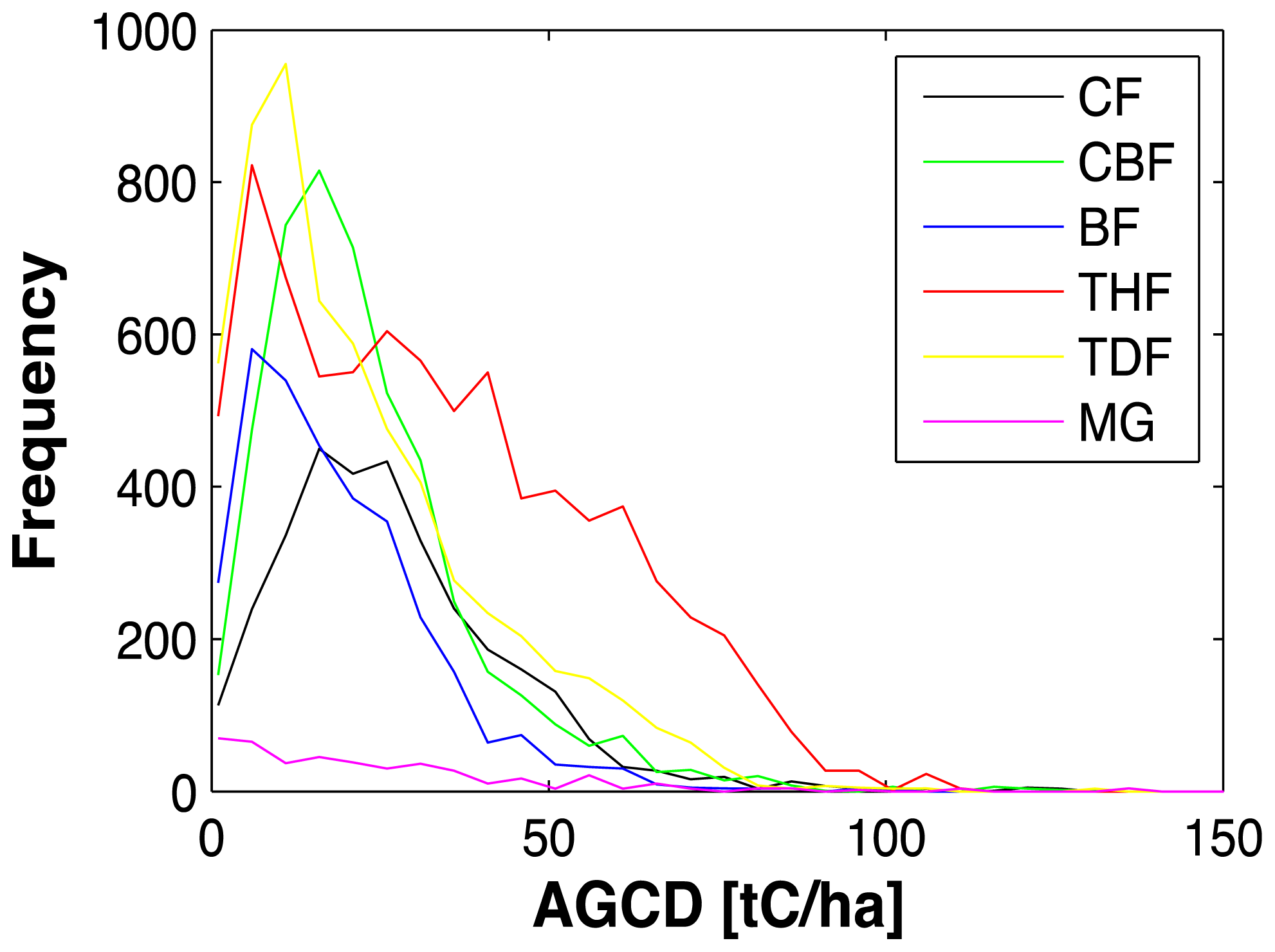
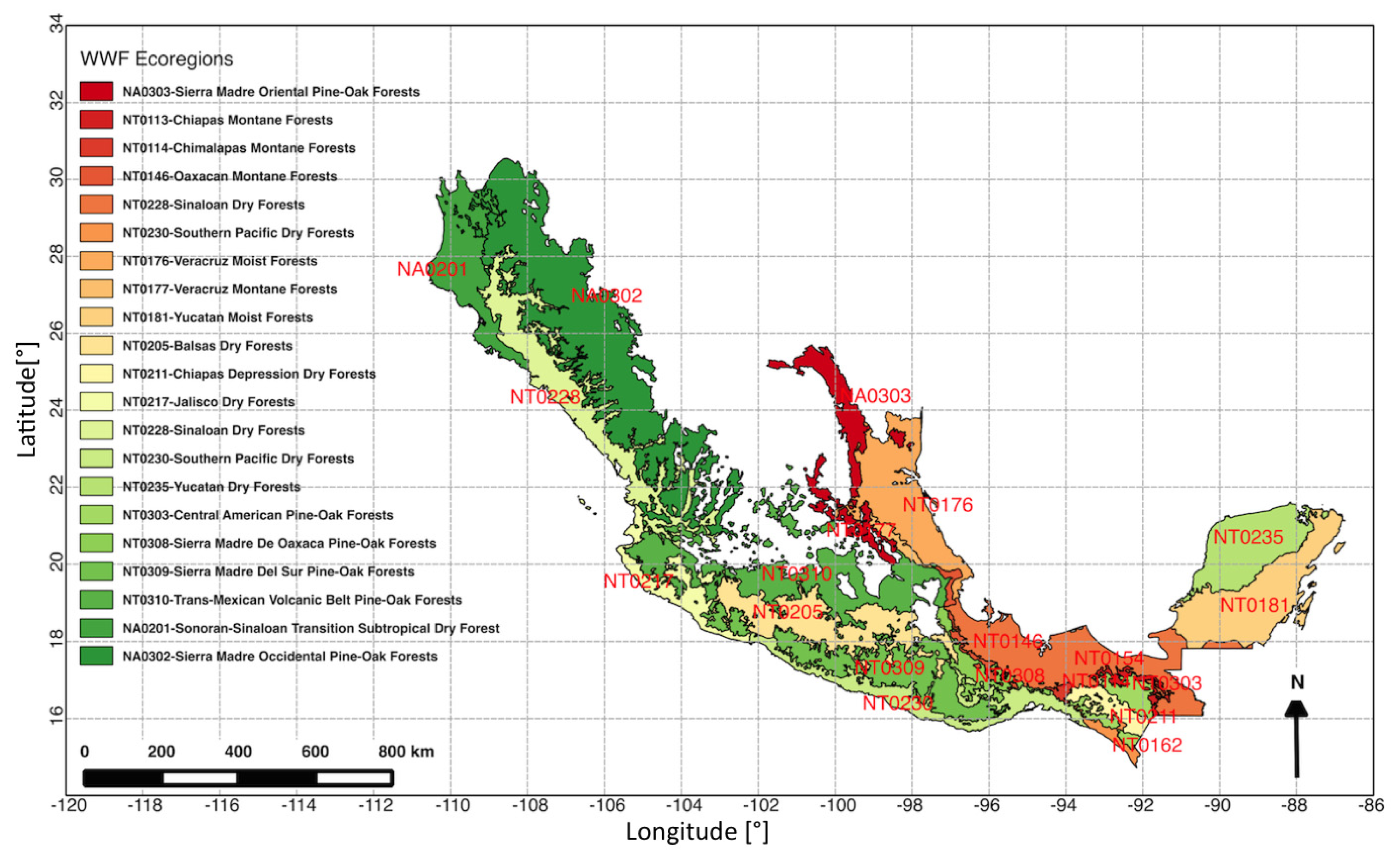
The average AGCD per state was calculated accordingly. The average AGCD in the map for each of the 32 states (including Distrito Federal) was calculated using as well the INEGI Series 4 land use map as a forest/non-forest mask. From INFyS plots, the average forest carbon stock per state was calculated as a weighted average of plot AGCD per forest type, using the proportion of the total state area covered by each forest type according to the INEGI land use map as weight. For plot stratification, forest types in the INEGI database were aggregated to six classes (Figure 1) to avoid specific forest types in a state to be only represented by a few plots; note that due to the lower number of plots, a stratification of plots per forest type was not feasible for the hexagon-scale comparison.

3. Results

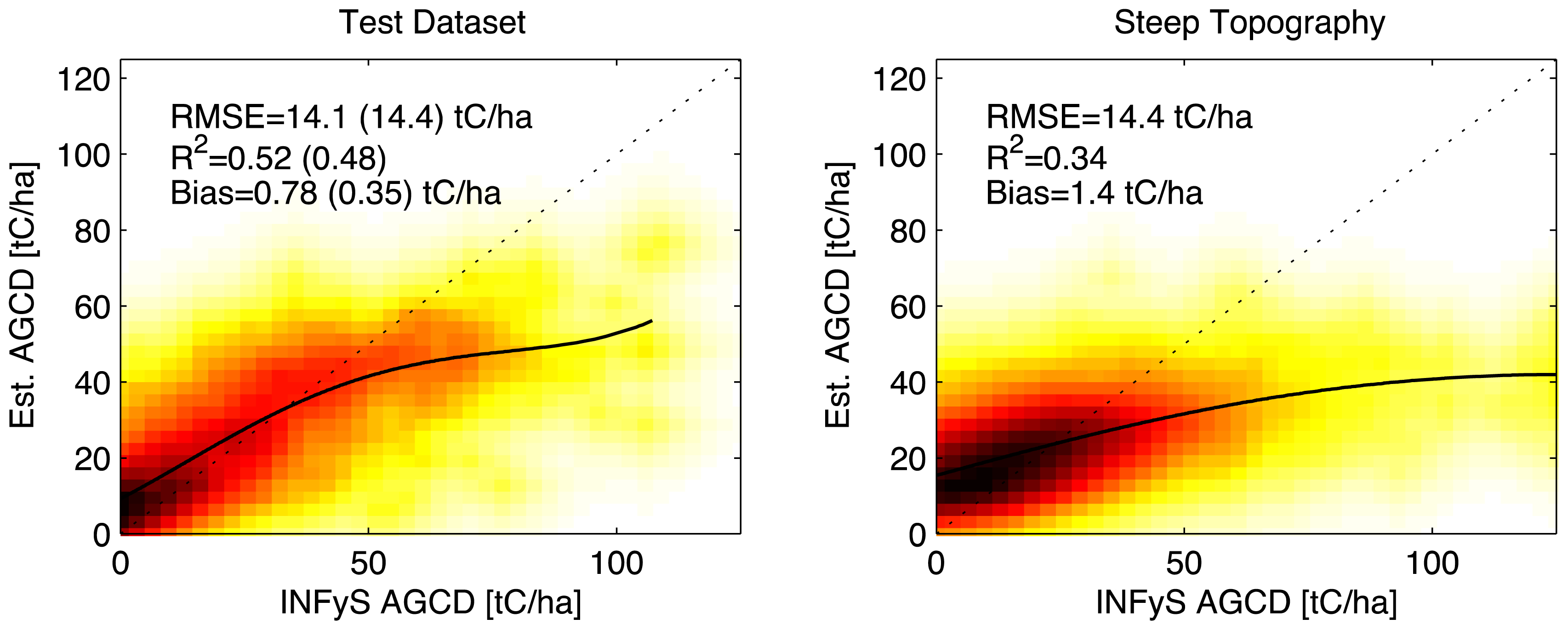
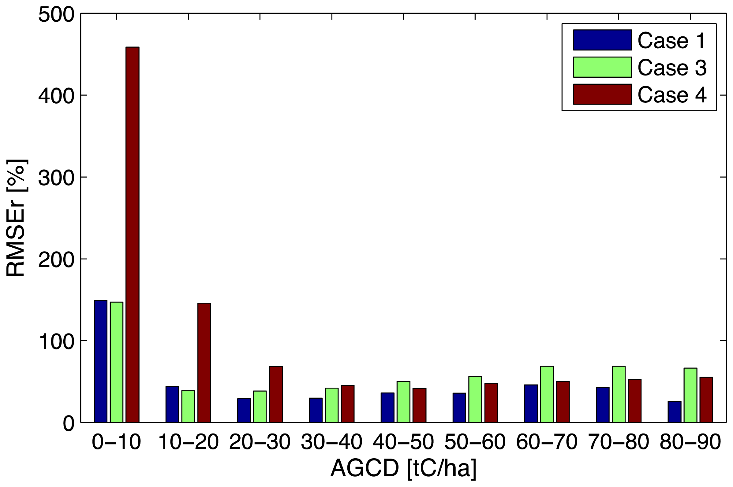
3.1. Model Performance

The performance of the AGCD retrieval when using all available optical, radar and ancillary predictor datasets in a single national-scale prediction model is illustrated in Figure 5. The figure shows the retrieval results for the INFyS plots that were part of: (1) the independent test dataset; and (2) the dataset comprising all plots located on steep slopes. Figure 5 also provides information on the RMSE, the R² as well as the bias. The OOB statistics are reported in parentheses. Overall, the results for the OOB predictions and the predictions for the independent test dataset were similar with an RMSE of ~14 t·C/ha (RMSEr of 54%), an R² of ~0.5 and a low bias of less than 1 t·C/ha, respectively. As indicated by the 4th order polynomial fit (black line in Figure 5), the predicted and INFyS AGCD were aligned along the 1:1 line for AGCDs up to about 40 to 50 t·C/ha. For AGCDs below 50 t·C/ha, the residuals were approximately normally distributed with a mean close to zero (2 t·C/ha); a tendency towards overestimation was observed for the lowest AGCDs. Conversely, for AGCDs above 50 t·C/ha, a clear tendency towards underestimation was observed. The predictions obtained for the plots located on steep slopes revealed a lower R² of 0.34 but similar RMSE of 14.4 t·C/ha (RMSEr of 63%). The estimation bias was also low for the predictions over steep terrain (1.4 t·C/ha).

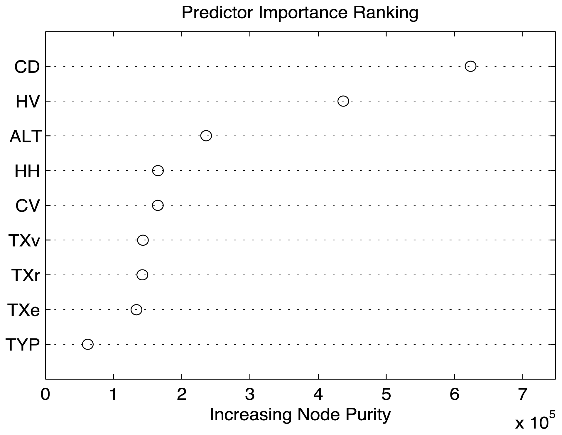
3.2. Predictor Importance

The randomForest predictor importance ranking (Figure 6), obtained by randomly permuting the values of a particular predictor and evaluating the change in the OOB retrieval accuracy [80], indicated that the Landsat canopy density was the most important predictor for the AGCD retrieval, followed by HV backscatter, SRTM elevation, and HH backscatter. The texture metrics and forest type information appeared to be of low importance for the retrieval performance.

To quantify for each forest type the contribution of different predictors to the overall retrieval performance, various model scenarios were assessed by excluding different variables from the predictor stack: Case (1) All available predictors used (benchmark); Case (2) Excluding forest type information; Case (3) Excluding PALSAR intensity and texture; Case (4) Excluding Landsat canopy density; Case (5) Excluding SRTM elevation. For each case scenario, one hundred randomForest models were trained each with a new stratified random selection of INFyS plots.

Figure 7 illustrates for each of the forest types the range (mean +/− standard deviation) of R², RMSE and bias for the predictions obtained for the independent test dataset. When using all predictors, the R² values were in the range of 0.5. Only for the MG class was the R² significantly lower (0.2). Average RMSE values were in a range of 11 t·C/ha (CBF, BF) to 21 t·C/ha (MG). The spread of accuracies between the different iterations was particularly large for MG. This was likely due to the much lower number of INFyS plots and an overall low sensitivity of the remote sensing datasets to the AGCD of MG. The estimation bias was consistently low (<1 t·C/ha) for all forest types. The exclusion of the INFyS forest type information had only a minor impact on the retrieval performance. For the CF, CBF, BF, THF, and MG classes, the range of the obtained R², RMSE as well as bias changed only marginally. Only in the case of TDF, the R² decreased for about 4% and the RMSE and bias increased for 1 and 2 t·C/ha, respectively. The exclusion of Landsat CD (i.e., the most important predictor according to randomForest) affected the retrieval performance for all forest types with decreases in R² between 7% (BF) and 20% (MG) and increases in RMSE in the range of 1 to 3 t·C/ha. The exclusion of the ALOS PALSAR datasets had an overall similar impact on the retrieval performance. For all forest classes, the exclusion of the PALSAR datasets resulted in a 4 (MG) to 14% lower R². Finally, the exclusion of the SRTM elevation was found to affect the retrieval performance for all forest types (3% to 10% lower R²) except MG (which is limited to low elevations).

The modeling with varying predictor combinations revealed systematic differences in the contribution of the radar and optical datasets in specific AGCD intervals. Figure 8 illustrates for the example of CBF that the retrieval accuracy (RMSEr) for plots with low AGCD < 20 t·C/ha appeared to depend mostly on Landsat CD since the RMSEr for the retrieval with all predictors (Case 1) and with Landsat CD and DEM (Case 3) produced similar results. For sparse forests with low AGCD, the retrieval error would have been much higher when using only PALSAR and DEM (Case 4). With increasing AGCDs, however, the retrieval increasingly depended on the PALSAR data.

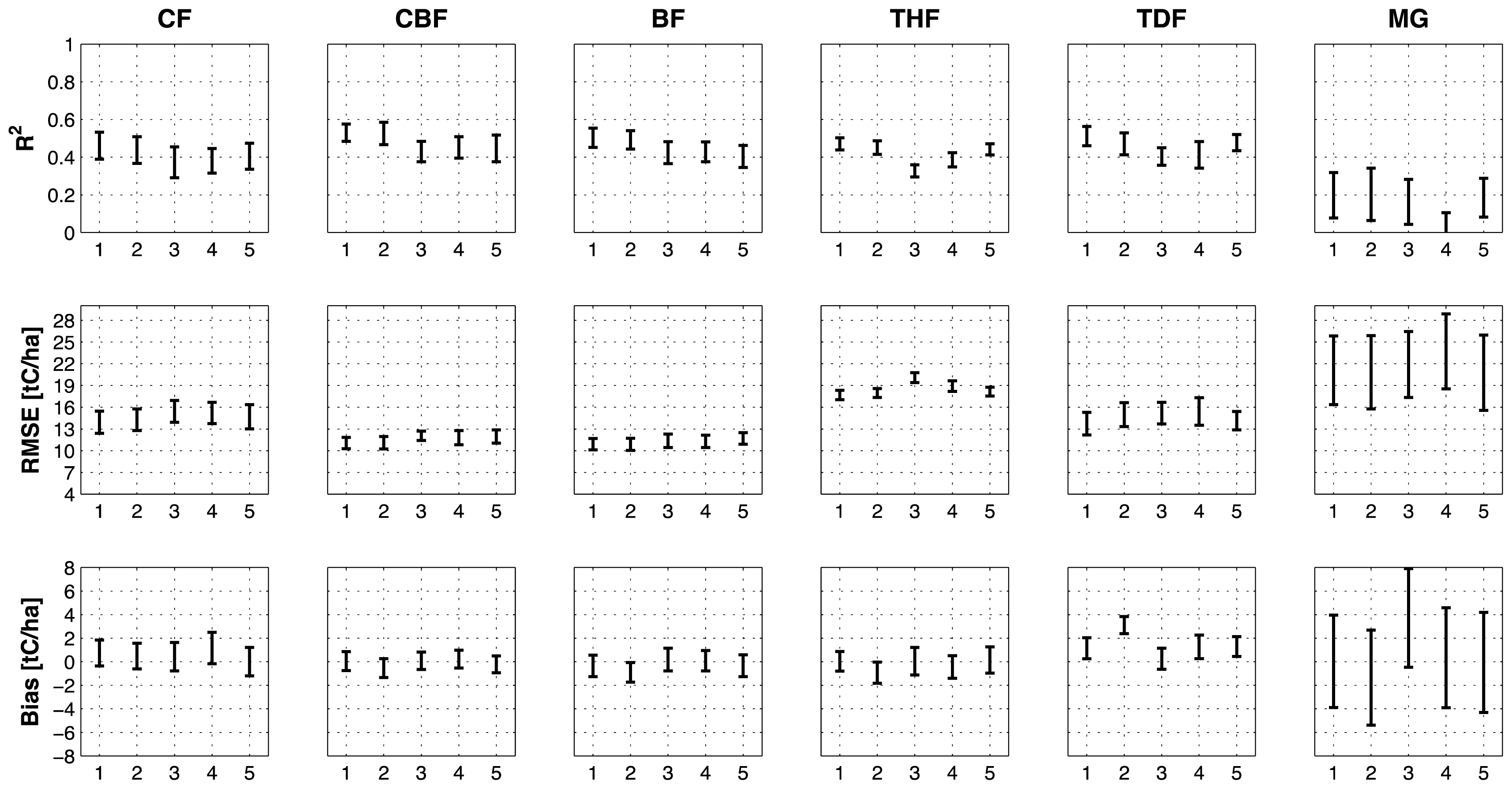
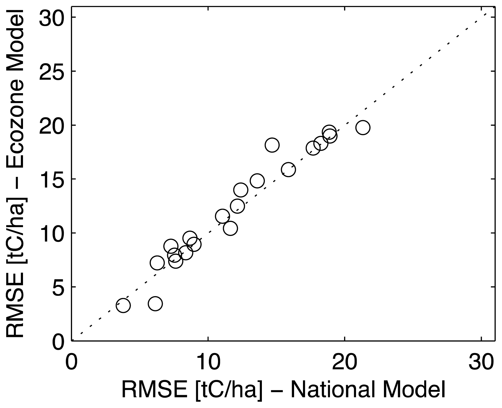
3.3. National Versus Ecoregional Modeling

Only minor differences were detected in the retrieval performance when predicting the AGCD for the plots in the independent test dataset using a national-scale model and models calibrated for each ecoregion, respectively (Figure 9). In each ecoregion, the AGCD predictions from the national and the ecoregional models were highly correlated and, when plotted against each other, aligned along the 1:1 line. In contrast to Kellndorfer et al. [11] or Blackard et al. [7], who implemented ecoregional modeling approaches to map the biomass across the United States using SRTM/Landsat and MODIS, respectively, we observed only minor differences in the predictor importance between the different ecoregions. Landsat CD and PALSAR HV were generally the most important predictors; HV backscatter ranked first for some of the pine-oak forest dominated ecoregions in the Sierra Madre Mountain range. As expected, the importance of elevation depended strongly on the topography in the respective ecoregions.

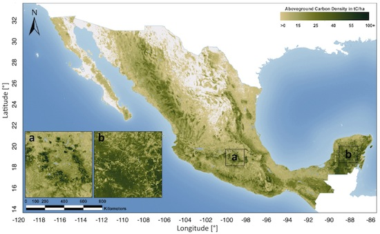
3.4. Wall-to-Wall AGCD Map

A wall-to-wall AGCD map with 30 × 30 m² pixel posting was produced using all available spatial datasets except forest type (see Section 4) as predictors in a single national-scale prediction model (Figure 10). According to the map, the highest carbon densities (> 50 t·C/ha) in Mexico can be found on the Yucatan Peninsula (Figure 10, inset b) as well as along the ridges of the Sierra Madre Del Sur and at the higher elevations of the Trans-Mexican Volcanic Belt (Figure 10, inset a). Because AGCD was predicted for all areas with a canopy density > 0% (Section-Modeling and Mapping), the map includes AGCD estimates for large portions of the arid wood/scrublands in Northern Mexico for which no biomass information was provided in the INFyS database (Section 2.1), i.e., for which strictly speaking the retrieval models were not appropriately calibrated. When applying a canopy density threshold of >0% to define forest, the total AGCD in Mexico according to the map was 2.21 Pg·C, which is 30% higher than the 1.69 Pg·C of forest aboveground carbon stocks that Mexico reported for the FAO Forest Resource Assessment 2010 [41] based on INFyS and the INEGI land use dataset and 38% higher than the 1.60 Pg·C that CONAFOR currently estimates based on the latest version of the INFyS and INEGI land use (Series V) data sets (unpublished CONAFOR draft report for FRA 2015). When using the INEGI land use map (Series 4) as a forest/non-forest mask, the total aboveground carbon stocks according to the map reduced to 1.53 Pg·C, which is only 4% below CONAFOR’s current estimate.

3.5. Multi-Scale Comparison of INFyS and Map

3.5.1. Hexagon-Scale Comparison

The per-hexagon differences between the AGCD estimates obtained from the remote sensing data and those from INFyS revealed a rather uniform distribution of over- and underestimation throughout the country (Figure 11). With an R² of 0.78 and an RMSE of 5 t·C/ha, the agreement between the per-hexagon AGCD estimates from INFyS and map was high. The differences between INFyS and predicted AGCD tended to increase from North to South, along with a general increase in AGCD from North to South. The Moran’s-I statistics indicated no clustering of over- or underestimation for most of the forest areas in Mexico. Significant (0.05 level) clustering was observed for the Southeast and parts of the Yucatan Peninsula, in particular. For the northwestern Yucatan, where dry tropical forests dominate, the observed AGCD estimates appeared to be systematically higher than the INFyS estimates. For the humid tropical forests of the southeastern Yucatan Peninsula (state of Quintana Roo), instead, AGCD appeared to be underestimated. As a consequence, the map in Figure 10 (inset b) presents a relatively constant carbon density across the Yucatan Peninsula, whereas the INFyS database reports a clear gradient with AGCD increasing from NW to SE. Some clustering was also observed for part of the mountain ranges (i.e., the Chiapas Highlands in Southern and the Sierra Madre Occidental in Northern Mexico).

3.5.2. State-Level Comparison

With a RMSE of 1.4 t·C/ha and a R² of 0.98, the comparison of the average carbon stocks according to the map and INFyS (Figure 12) at the state-level confirmed that the up-scaling of INFyS to a wall-to-wall map with the remote sensing imagery preserved the major patterns in the distribution of the aboveground carbon stocks across Mexico. As for the hexagon-scale comparison, the biggest difference (−4 t·C/ha) between map and INFyS was observed for Quintana Roo, Yucatan Peninsula.

3.6. Results in the Context of Published Accuracy Requirements

The scientific community has published accuracy requirements for biomass and carbon stock estimation in the recent past. Hall et al. [1] suggested that a retrieval error for biomass of better than 20% or 20 t/ha (i.e., an AGCD of ~10 t·C/ha), respectively, for aboveground biomasses below 100 t/ha and for at least 80% of predictions at the hectare scale would be required to reduce the current uncertainty in the terrestrial carbon budget to a level comparable to that associated with the oceanic carbon uptake. Dependent on the forest type, the estimates for Mexico were within the 20%/10 t·C/ha range for 52% to 76% of 1 hectare INFyS plots (test dataset) with an AGCD below 50 t·C/ha located on flat terrain (CF: 74%, CBF: 76%, BF: 74%, THF: 52%, TDF: 70%, MG: 54%); the requirements were fulfilled for 49 to 67% of the INFyS plots located on steep terrain (CF: 63%, CBF: 65%, BF: 67%, THF: 49%, TDF: 70%).

4. Discussion

The modeling approach and map presented here for Mexico demonstrate both the potential as well as limitations of the fusion of contemporary, globally available spaceborne datasets for large-scale mapping of aboveground biomass and associated carbon stocks at medium spatial resolutions. The results clearly show the benefit of radar/optical fusion as with either data set alone, the retrieval performance would have been significantly reduced. The comparison against INFyS and remote sensing predictions at different spatial scales (plots, hexagons, states) showed that a single national-scale prediction model, with few regional exceptions (Figure 11), allowed the mapping of forest aboveground carbon stocks without significant regional biases. However, at the scale of the INFyS plots (i.e., the hectare scale), the uncertainty of the AGCD predictions is large and retrieval accuracies postulated by the scientific community [1] at this spatial scale are not met. Higher retrieval accuracies at the hectare scale with L-band radar and multi-spectral optical imagery have been reported in the literature for smaller study areas [40]. The results for Mexico hence demonstrate the limitations associated with mapping forest aboveground biomass across a large number of images, varying imaging conditions and diverse forest ecosystems.

Landsat data, in the form of a canopy density product, was an important predictor for the aboveground biomass of forests in Mexico (Figure 6). Optical remote sensing based estimates of canopy density have been used to predict forest biophysical attributes such as height, growing stock volume, and aboveground biomass for forests in the US [11,36], for tropical forests in the Amazon [12], for boreal forests in Sweden and Central Siberia [81], as well as for an arid forest area in North Central Mexico [82]. A limitation of canopy density metrics as predictors of aboveground biomass is that they function well only as long as the canopies are not closed (i.e., primarily during early-successional stages of forest development). Biomass differences between forests with closed canopies are not captured [81]. Recent studies focused on large-area mapping of aboveground biomass in the tropics with passive optical imagery (Landsat, MODIS) have suggested that there is sensitivity in optical imagery (Landsat, MODIS) to aboveground biomass beyond the correlation of biomass and percent canopy cover, which essentially derives from the spectral contrast between the tree canopies and the underlying forest floor. In particular, the short wave infrared (SWIR) bands, which are most sensitive to canopy moisture differences and shadowing effects, have been found to be sensitive to aboveground biomass even for forests with closed canopies [10,17]. The results of these studies suggest that the biomass retrieval for Mexico can be further improved by adding actual Landsat reflectance data to the predictor stack. In particular in the tropical regions of Mexico, where cloud cover is persistent, the creation of radiometrically consistent seasonal or even monthly reflectance mosaics is a complex task that typically requires imagery from multiple years. The creation of such mosaics was beyond the scope of this study.

In theory, the sensitivity of L-band backscatter to aboveground biomass should exceed that of (optical) canopy density metrics since the backscatter from forest is not only governed by the extent of gaps (i.e., canopy density) but also the depth and vertical structure of the canopy; note that a relatively simple way of modeling backscatter from forest is to consider the measured backscatter a sum of backscatter from forest floor and canopy weighted by the gap extent and the signal attenuation within the canopy, with the latter being a function of the canopy height [83]. However, this study found that PALSAR backscatter measurements in co- and cross-polarization (HH, HV) were overall less correlated to AGCD than the Landsat derived canopy density estimates (Pearson correlation for different forest types of AGCD and HV: 0.22–0.54, HH: 0.18–0.47, VCF: 0.5–0.58) and hence, with few regional exceptions (Section 3.3), ranked lower in the randomForest importance ranking (Figure 6). This was most likely a consequence of the sensitivity of the radar measurements to environmental factors, most prominently soil and canopy moisture variations at stand- to landscape-scales that have been shown to affect the form and strength of the relationship between the backscatter measurements and forest biophysical attributes [19,29,66,68,72,73,84]. Model investigations in Wang et al. [85] indicated that also other factors (forest floor roughness, litter depth) could introduce significant variability in L-band observations of forest, in particular at HH polarization. The retrieval of forest biophysical parameters based on L-band data generally performs best when the effect of moisture variations in soils and vegetation are minimized, for instance in arid regions or during extended dry periods [30,84]. As discussed in Lucas et al. [29], the limited availability of multi-temporal observations from ALOS PALSAR hampers the possibility to generate large-area ALOS PALSAR L-band backscatter mosaics that consistently represent dry conditions. ALOS PALSAR locally acquired between one and five dual-polarization images per year [86]. In the case of Mexico, only few images had to be adjusted radiometrically to generate mosaics without major banding effects. The fact that radar backscatter was less correlated to AGCD than optically based canopy density estimates suggests, however, that local variations in PALSAR imaging conditions (beyond the landscape scale moisture variations that show up in mosaics as stripes) affected the radar’s performance in the retrieval, in particular for sparse forests with low biomass (Figure 8).

Significant improvements in the retrieval performance with L-band radar have been reported when integrating multi-temporal radar observations, either as additional predictors or by combining estimates obtained for each image in a multi-temporal stack [19,35,39,71,72,87], as with multi-temporal stacks of data the influence of environmental effects, as well as the radar inherent speckle noise, can be reduced. The results in [19] indicated, for the Northeastern United States, that aboveground biomass could be mapped consistently up to biomass levels of ~180 t/ha when having at least four PALSAR dual-polarization L-band acquisitions. Because of the lack of a consistent multi-temporal PALSAR coverage, multi-temporal retrieval approaches such as those presented in [15,19] for C- and L-band, respectively, could not be implemented in the case of Mexico. It remains to be seen whether the limitations associated with the multi-temporal acquisition strategy of ALOS PALSAR will be overcome in the coming years with the launch of the next generation L-Band SAR missions: the Japanese mission, ALOS-2 (launch 2014), the Argentinian SAOCOM mission (launch 2017), and the planned NASA/ISRO L-band/S-band radar mission (launch 2020).

Recently published studies showed that texture metrics derived from radar imagery correlate with forest attributes such as stand age or aboveground biomass [88,89]. The results of these studies suggested that the use of texture metrics jointly with backscatter measurements could improve the biomass retrieval performance. In the case of Mexico, however, texture metrics derived from L-band radar hardly contributed to the overall retrieval performance (Figure 6). On one side, this might be explained with the limited number of texture metrics that were computed (cf., [89]). However, the promising results in [88,89] were achieved for smaller test sites and a limited number of field plots. It remains unclear how consistent the relationship between texture metrics and aboveground biomass is across a large number of images, varying imaging conditions and heterogeneous forest ecosystems.

In the case of Mexico, the low sensitivity of the available optical and radar datasets to differences in AGCD beyond ~50 t·C/ha was somewhat counterbalanced by the fact that in mountainous regions, the biomass increases with increasing elevation (because of concurrent increases in annual precipitation) so that AGCDs above 50 t·C/ha could be predicted with the aid of a DEM (Figure 10, inset a). In areas with high biomass densities at low elevations, foremost in parts of the Yucatan Peninsula, high AGCD ranges were instead underestimated (Figure 11). On the other hand, overestimation of AGCD was observed specifically for the dry tropical forests of the Yucatan Peninsula even though, for dry tropical forests across the entire country, the retrieval accuracy was comparable to other forest classes (Figure 7). An explanation for the overestimation of the dry tropical forest’s biomass on the Yucatan could be seasonal leaf-on/loaf-off effects in the Landsat VCF product. A comparison of INFyS AGCD and Landsat canopy density showed locally very high canopy densities for plots with low AGCD according to INFyS, which was not observed for similar types of forests in other parts of the country. A contributing factor may have been the limited Landsat data availability over the tropical parts of Mexico where cloud cover tends to be persistent. The overall lowest retrieval accuracy (R² of 0.2) was achieved for mangroves, a forest type that due to permanent or periodic flooding presents distinct characteristics in remote sensing imagery. L-band radar has shown some potential for the mapping of aboveground biomass of mangroves [90]. The results here, however, indicate that a simple national-scale modeling approach is underperforming for the retrieval of mangrove biomass.

In contrast to other studies [17,36], the inclusion of forest type information in the biomass retrieval did not improve the retrieval performance significantly. While in some forested ecoregions, forest types readily explain biomass differences, Mexico presents a complex environmental setting where variations in aboveground biomass due to environmental factors like precipitation, forest management practices, and disturbance regimes [91,92] are more pronounced than the differences in biomass between most of the major forest types (Figure 1). Also, the INEGI maps for Mexico at the scale of 1:250,000 are rather generalized, and imply significant uncertainty at the hectare-scale targeted for the mapping of AGCD across Mexico. It therefore appeared preferable not to use the INEGI land use maps for the production of the biomass map of Mexico.

The pre-processing of the remote sensing datasets that were used to map AGCD across Mexico utilized state-of-the-art methods for geocoding, ortho-rectification and signal calibration. For the generation of the Landsat canopy density product [46], for instance, USGS Level 1 terrain-corrected (L1T) Landsat ETM+ data had been used, for which radiometric calibration and geometric corrections were applied using a DEM. For the pre-processing of the ALOS PALSAR data, a new approach for compensating for the dependence of the pixel scattering area contributing to the measured backscatter on topography was applied that has been shown to allow significant improvements in the calibration of radar data over mountainous terrain compared to previously developed approaches when having a DEM with a spatial resolution comparable to that of the radar imagery [56,93]. However, due to licensing restrictions for use at non US government facilities only SRTM 3-arcsec data were available to calibrate the SAR data in Mexico, which contributed to a lower accuracy of the AGCD estimates over steep terrain. Regionally, geo-location inaccuracies in the INFyS plot database might have contributed to the reduced biomass retrieval performance over steep terrain. Overall, the results showed, however, that topographic distortions over steep terrain are still a significant constraint for large area mapping applications, at least without DEMs with a spatial resolution on the order or better than the remote sensing imagery to correct for topographic effects.

Although nominally providing sub-hectare scale information on aboveground carbon density, the map will be of limited use for stand-level analysis of aboveground carbon stocks. However, in particular in the context of the ongoing preparations in Mexico for putting in place a REDD+ MRV system, the map is expected to provide valuable information on forest carbon stocks at spatial scales (e.g., communal, municipal) at which the number of INFyS plots will be insufficient to produce localized estimates of carbon stocks. To evaluate whether the spatially explicit map is a viable alternative to “Stratify and Multiply” [94] approaches, i.e., in the case of Mexico an extrapolation of INFyS with the aid of land cover products such as the INEGI products, it is necessary to quantify the map uncertainty at different spatial scales. Different error sources that propagate to the final per-pixel estimates of AGCD in the map have to be considered: (i) field measurements; (ii) allometric equations, (iii) sampling error; (iv) remote sensing predictions. The time difference between the collection of the INFyS inventory (2004–2007), and acquisition of the Landsat (2000–2004) and ALOS PALSAR data sets (2007) also has to be acknowledged as a possible local source of uncertainty. The largest uncertainty is associated with the remote sensing predictions. Dependent on the biomass level (Figure 8), the error at the plot-level is between 30% and 150%. The uncertainty related to the field (i.e., DBH) measurements can be expected to be low since DBH measurement errors for single trees tend to average out when summing over all trees in a plot. Given the large number of plots in the Mexican NFI, the sampling error can also be expected to be low [95]. The uncertainty related to the set of allometric equations (cf. Section 2.1) that were used to estimate aboveground carbon density from in situ DBH measurements has not yet been assessed. The allometric error should be in the range of 10% to 30% [52,95]. Future work will address, in collaboration with CONAFOR, the propagation of errors associated with the inventory data and remote sensing predictions at the plot level as well as the spatial propagation of errors when aggregating the pixel estimates to coarser scales [96], with a particular focus on scales relevant for the Mexican MRV system (i.e., communal, municipal).

5. Conclusions and Outlook

A first spatially explicit map of the aboveground biomass and carbon stocks of forests across Mexico with 30 m pixel posting was produced. The map provides decision makers and land managers in Mexico a new tool for forest resource management and carbon stock assessment at spatial scales at which the density of field plots in the national forest inventory database is too sparse. The map will be publicly available.

The results of this study demonstrate that the fusion of medium resolution optical and dual-polarization L-band data augmented by geophysical gradient information (i.e., a DEM), all of which are available globally and will also be in the foreseeable future (ALOS-2, SAOCOM, NASA/ISRO DESDynI-R, Landsat-8), provides a relatively straightforward, off-the-shelf approach for extending plot-level forest inventory estimates of aboveground biomass to spatially explicit large-area maps. While the benefit of fusing medium resolution L-band radar and optical datasets for mapping forest biomass and carbon stocks has been demonstrated for smaller study areas [40], our results here show that radar/optical fusion allows for consistent improvements in the retrieval performance when mapping across large areas and a wide range of temperate, sub-tropical and tropical forest types. Furthermore, we were able to show that radar/optical fusion is particularly beneficial in the case of sparse forests with low biomass (<20 t·C/ha) for which the radar backscatter is strongly affected by variations in the environmental imaging conditions (most prominently soil moisture variations). A comparison of the average carbon stocks computed from: (a) the map; and (b) statistical estimates from the national forest inventory for ~650 km² large hexagons and Mexican states, showed that a single national-scale prediction model allows the mapping of the distribution of aboveground carbon stocks across diverse forest ecosystems without significant regional biases.

The map should be regarded first and foremost as a tool for carbon stock assessments at the jurisdictional (e.g., communal, municipal) level. With about 50% of biomass variability being explained in the case of forests located on flat terrain and even less in the case of mountainous terrain, the limitations of the map at the hectare scale (i.e., the scale of anthropogenic and natural disturbance) emphasize the need for exploring additional data sources and methods to complement the national dataset with more accurate information on local forest condition, biomass, and carbon stocks. In the frame of the USAID funded Mexico-REDD+ project [97] airborne lidar transects are therefore currently (years 2013/14) being acquired in six critical forest areas across Mexico (Yucatan, Chiapas, Oaxaca, Michoacán, Jalisco, Chihuahua). Also, in April/May 2013, the AMIGA lidar campaign acquired transects of lidar data with the NASA G-LiHT sensor [98]. The lidar data will provide additional means to: (i) investigate forest structural and carbon stock differences related to disturbance and forest management; and (ii) improve AGCD mapping by extending field inventory data via lidar transects to wall-to-wall maps [20,39,40] using new spaceborne remote sensing datasets from the Landsat-8 optical or the soon to be launched ALOS-2 and SENTINEL-1 L- and C-band radar missions. Lidar transects will also be acquired over mangrove forest sites to investigate alternative options for Mexico to quantify mangrove biomass, which is not well represented in the produced biomass map.

References

1. Hall, F.G.; Bergen, K.; Blair, J.B.; Dubayah, R.; Houghton, R.; Hurtt, G.; Kellndorfer, G.; Lefsky, M.; Ranson, J.; Saatchi, S.; et al. Characterizing 3D vegetation structure from space: Mission requirements. Remote Sens. Environ 2011, 115, 2753–2775. [Google Scholar]
2. Birdsey, R.; Angeles-Perez, G.; Kurz, W.A.; Lister, A.; Olguin, M.; Pan, Y.; Wayson, C.; Wilson, B.; Johnson, K. Approaches to monitoring changes in carbon stocks for REDD+. Carbon Manag 2013, 4, 519–537. [Google Scholar]
3. Jantz, P.; Goetz, S.; Laporte, N. Carbon stock corridors to mitigate climate change and promote biodiversity in the tropics. Nat. Clim. Chang 2014, 4, 138–142. [Google Scholar]
4. Hansen, M.C.; de Fries, R.S.; Townshend, J.R.G.; Carroll, M.; Dimiceli, C.; Sohlberg, R.A. Global percent tree cover at a spatial resolution of 500 meters: First results of the MODIS Vegetation Continuous Field algorithm. Earth Interact 2003, 7, 1–15. [Google Scholar]
5. Reese, H.; Nilsson, M.; Granqvist Pahlén, T.; Hagner, O.; Joyce, S.; Tingelöf, U.; Egberth, M.; Olsson, H. Countrywide estimates of forest variables using satellite data and field data from the National Forest Inventory. Ambio 2003, 32, 542–548. [Google Scholar]
6. Wagner, W.; Luckman, A.; Vietmeier, J.; Tansey, K.; Balzter, H.; Schmullius, C.; Davidson, M.; Gaveau, D.; Gluck, M.; Le Toan, T.; et al. Large-scale mapping of boreal forest in SIBERIA using ERS tandem coherence and JERS backscatter data. Remote Sens. Environ 2003, 85, 125–144. [Google Scholar]
7. Blackard, J.A.; Finco, M.V.; Helmer, E.H.; Holden, G.R.; Hoppus, M.L.; Jacobs, D.M.; Lister, A.J.; Moisen, G.G.; Nelson, M.D.; Riemann, R.; et al. Mapping US forest biomass using nationwide forest inventory data and moderate resolution information. Remote Sens. Environ 2008, 112, 1658–1677. [Google Scholar]
8. Boudreau, J.; Nelson, R.; Margolis, H.; Beaudoin, A.; Guindon, L.; Kimes, D. Regional aboveground forest biomass using airborne and spaceborne LiDAR in Québec. Remote Sens. Environ 2008, 112, 3876–3890. [Google Scholar]
9. Lefsky, M.A. A global forest canopy height map from the Moderate Resolution Imaging Spectroradiometer and the Geoscience Laser Altimeter System. Geophys. Res. Lett 2010, 37, 1–5. [Google Scholar]
10. Baccini, A.; Goetz, S.; Walker, W.; Laporte, N.; Sun, M.; Sulla-Menashe, D.; Hackler, J.; Beck, P.S.A.; Dubayah, R.; Friedl, M.A.; et al. Estimated carbon dioxide emissions from tropical deforestation improved by carbon-density maps. Nat. Clim. Chang 2012, 2, 1–4. [Google Scholar]
11. Kellndorfer, J.; Walker, W.; LaPoint, E.; Bishop, J.; Cormier, T.; Fiske, G.; Hoppus, M.; Kirsch, K.; Westfall, J. NACP Aboveground Biomass and Carbon Baseline Data (NBCD 2000), USA, 2000; Oak Ridge National Laboratory Distributed Active Archive Center (ORNL DAAC): Oak Ridge, TN, USA, 2012. [Google Scholar]
12. Saatchi, S.S.; Houghton, R.A.; Dos Santos Alvalá, R.C.; Soares, J.V.; Yu, Y. Distribution of aboveground live biomass in the Amazon basin. Glob. Chang. Biol 2007, 13, 816–837. [Google Scholar]
13. Saatchi, S.S.; Harris, N.; Brown, S.; Lefsky, M.; Mitchard, E.T.; Salas, W.; Zutta, B.R.; Buerman, W.; Lewsi, S.L.; Hagen, S.; et al. Benchmark map of forest carbon stocks in tropical regions across three continents. Proc. Natl. Acad. Sci.USA 2011, 108, 9899–9904. [Google Scholar]
14. Simard, M.; Pinto, N.; Fisher, J.B.; Baccini, A. Mapping forest canopy height globally with spaceborne lidar. J. Geophys. Res 2011, 116, 1–12. [Google Scholar]
15. Santoro, M.; Beer, C.; Cartus, O.; Schmullius, C.C.; Shvidenko, A.; McCallum, I.; Wegmüller, U.; Wiesmann, A. Retrieval of growing stock volume in boreal forest using hyper-temporal series of Envisat ASAR ScanSAR backscatter measurements. Remote Sens. Environ 2011, 115, 490–507. [Google Scholar]
16. Santoro, M.; Cartus, O.; Fransson, J.; Shvidenko, A.; McCallum, I.; Beaudoin, A.; Hall, R.; Beer, C.; Schmullius, C. Estimates of forest growing stock volume estimates for Sweden, Central Siberia and Quebec using Envisat Advanced Synthetic Aperture Radar backscatter data. Remote Sens 2013, 5, 4503–4532. [Google Scholar]
17. Avitabile, V.; Baccini, A.; Friedl, M.A.; Schmullius, C.C. Capabilities and limitations of Landsat and land cover data for aboveground woody biomass estimation of Uganda. Remote Sens. Environ 2012, 117, 366–380. [Google Scholar]
18. Cartus, O.; Santoro, M.; Schmullius, C.C.; Li, Z. Large area forest stem volume mapping in the boreal zone using synergy of ERS-1/2 tandem coherence and MODIS vegetation continuous fields. Remote Sens. Environ 2011, 115, 931–943. [Google Scholar]
19. Cartus, O.; Santoro, M.; Kellndorfer, J. Mapping of forest aboveground biomass in the northeastern United States with ALOS PALSAR dual-polarization L-band. Remote Sens. Environ 2012, 124, 466–478. [Google Scholar]
20. Baccini, A.; Asner, G. Improving pantropical forest carbon maps with airborne lidar sampling. Carbon Manag 2013, 4, 591–600. [Google Scholar]
21. Guindon, L.; Beaudoin, A.; Leboeuf, A.; Ung, C.H.; Luther, J.E.; Côté, S.; Lambert, M.C. Regional mapping of Canadian Subarctic Forest Biomass Using a Scaling up Method Combining QuickBird and Landsat Imagery. Proceedings of the 2005 ForestSAT Symosium, Borås, Sweden, 31 May–1 June 2005; pp. 71–75.
22. Asner, G.; Clark, J.K.; Mascaro, J.; Galindo Garcia, G.A.; Chadwick, K.D.; Navarette Encinales, D.A.; Paez-Acosta, G.; Montenegro, C.; Kennedy-Bowdoin, T.; Duque, A.; et al. High-resolution mapping of forest carbon stocks in the Colombian Amazon. Biogeosciences 2012, 9, 2683–2696. [Google Scholar]
23. Le Toan, T.; Beaudoin, A.; Riom, J.; Guyon, D. Relating forest biomass to SAR data. IEEE Trans. Geosci. Remote Sens 1992, 30, 403–411. [Google Scholar]
24. Dobson, M.C.; Ulaby, F.T.; Le Toan, T.; Beaudoin, A.; Kasischke, E.S.; Christensen, N. Dependence of radar backscatter on coniferous forest biomass. IEEE Trans. Geosci. Remote Sens 1992, 30, 412–415. [Google Scholar]
25. Ranson, K.J.; Sun, G. Mapping biomass of a northern forest using multifrequency SAR data. IEEE Trans. Geosci. Remote Sens 1994, 32, 388–396. [Google Scholar]
26. Imhoff, M. Radar backscatter and biomass saturation: Ramifications for global biomass inventory. IEEE Trans. Geosci. Remote Sens 1995, 33, 511–518. [Google Scholar]
27. Ranson, K.J.; Saatchi, S.S.; Sun, G. Boreal forest ecosystem characterization with SIR-C/XSAR. IEEE Trans. Geosci. Remote Sens 1995, 33, 867–876. [Google Scholar]
28. Lucas, R.M.; Cronin, N.; Lee, A.; Moghaddam, M.; Witte, C.; Tickle, P. Empirical relationships between AIRSAR backscatter and LiDAR-derived forest biomass, Queensland, Australia. Remote Sens. Environ 2006, 100, 407–425. [Google Scholar]
29. Lucas, R.M.; Armston, J.; Fairfax, R.; Fensham, R.; Accad, A.; Carreiras, J.; Kelley, J.; Bunting, P.; Clewley, D.; Bray, S.; Metcalfe, D.; et al. An evaluation of the ALOS PALSAR L-band backscatter—Above ground biomass relationship Queensland, Australia: Impacts of surface moisture condition and vegetation structure. IEEE J. Sel. Top. Appl. Earth Observ 2010, 3, 576–593. [Google Scholar]
30. Mitchard, E.T.A.; Saatchi, S.S.; Woodhouse, I.H.; Nangendo, G.; Ribeiro, N.S.; Williams, M.; Ryan, C.M.; Lewis, S.L.; Feldpausch, T.R.; Meir, P. Using satellite radar backscatter to predict above-ground woody biomass: A consistent relationship across four different African landscapes. Geophys. Res. Lett 2009, 36, 1–6. [Google Scholar]
31. Sandberg, G.; Ulander, L.M.H.; Fransson, J.E.S.; Holmgren, J.; Le Toan, T. L- and P-band backscatter intensity for biomass retrieval in hemiboreal forest. Remote Sens. Environ 2011, 115, 2874–2886. [Google Scholar]
32. Le Toan, T.; Quegan, S.; Davidson, M.; Balzter, H.; Paillou, P.; Papathanassiou, K.; Plummer, S.; Rocca, F.; Saatchi, S.; Shugart, H.; et al. The BIOMASS mission: Mapping global forest biomass to better understand the terrestrial carbon cycle. Remote Sens. Environ 2011, 115, 2850–2860. [Google Scholar]
33. Papathanassiou, K.P.; Cloude, S.R. Single-baseline polarimetric SAR interferometry. IEEE Trans. Geosci. Remote Sens 2001, 39, 2352–2363. [Google Scholar]
34. Reigber, A.; Moreira, A. First demonstration of airborne SAR tomography using multibaseline L-band data. IEEE Trans. Geosci. Remote Sens.
35. Rauste, Y. Multi-temporal JERS SAR data in boreal forest biomass mapping. Remote Sens. Environ 2005, 97, 263–275. [Google Scholar]
36. Walker, W.; Kellndorfer, J.M.; Lapoint, E.; Hoppus, M.; Westfall, J. An empirical InSAR-optical fusion approach to mapping vegetation canopy height. Remote Sens. Environ 2007, 109, 482–499. [Google Scholar]
37. Kellndorfer, J.; Walker, W.; LaPoint, E.; Kirsch, K.; Bishop, J.; Fiske, G. Statistical fusion of lidar, InSAR, and optical remote sensing data for forest stand height characterization: Regional-scale method based on LVIS, SRTM, Landsat ETM+, and ancillary data sets. J. Geophys. Res 2010, 115, 1–10. [Google Scholar]
38. Andersen, H.E.; Strunk, J.; Temesgen, H.; Atwood, D.; Winterberger, K. Using multilevel remote sensing and ground data to estimate forest biomass resources in remote regions: A case study in boreal forests of interior Alaska. Can. J. Remote Sens 2011, 37, 596–611. [Google Scholar]
39. Cartus, O.; Kellndorfer, J.; Rombach, M.; Walker, W. Mapping canopy height and growing stock volume using airborne Lidar, ALOS PALSAR and Landsat ETM+. Remote Sens 2012, 4, 3320–3345. [Google Scholar]
40. Montesano, P.M.; Cook, B.D.; Sun, G.; Simard, M.; Nelson, R.F.; Ranson, K.J.; Zhang, Z.; Luthcke, S. Achieving accuracy requirements for forest biomass mapping: A spaceborne data fusion method for estimating forest biomass and LiDAR sampling error. Remote Sens. Environ 2013, 130, 153–170. [Google Scholar]
41. Food and Agriculture Organization (FAO), Evaluación de los Recursos Forstales Mundiales 2010—Informe Nacional México; FAO: Rome, Italy, 2010.
42. The National Forestry Commission of Mexico (CONAFOR), Inventario Nacional Forestal u de Suelos Informe 2004–2009; CONAFOR: Zapopan, México, 2012.
43. The National Commission for the Knowledge and Use of Biodiversity (CONABIO), Capital Natural y bienestar Social. Comisión Nacional para el Conocimiento y Uso de la Biodiversidad; CONABIO: Zapopan, México, 2006.
44. Kellndorfer, J.; Walker, W.; Pierce, L.E.; Dobson, M.C.; Fites, J.; Hunsaker, C.; Vona, J.; Clutter, M. Vegetation height estimation from Shuttle Radar Topography Mission and National Elevation Datasets. Remote Sens. Environ 2004, 93, 339–358. [Google Scholar]
45. Walker, W.; Kellndorfer, J.; Pierce, L. Quality assessment of SRTM C- and X-band interferometric data: Implications for the retrieval of vegetation canopy height. Remote Sens. Environ 2007, 106, 428–448. [Google Scholar]
46. Hansen, M.C.; Egorov, A.; Roy, D.P.; Potapov, P.; Ju, J.; Turubanova, S.; Kommareddy, I.; Loveland, T.R. Continuous fields of land cover for the conterminous United States using Landsat data: First results from the Web-Enabled Landsat Data (WELD) project. Remote Sens. Lett 2011, 2, 279–288. [Google Scholar]
47. Instituto Nacional de Estadística y Geografía (INEGI), Conjunto Nacional de Uso del Suelo y Vegetación a escala 1:250,000, Serie IV; DGG-INEGI: Aguascalientes, México, 2010.
48. De Jong, B.H.J.; Anaya, C.; Masera, O.; Olguín, M.; Paz, F.; Etchevers, J.; Martínez, R.D.; Guerrero, G.; Balbontín, C. Greenhouse gas emissions between 1993 and 2002 from land-use change and forestry in Mexico. For. Ecol. Manag 2010, 260, 1689–1701. [Google Scholar]
49. Bechtold, W.A.; Patterson, P.L. The Enhanced Forest Inventory and Analysis Program—National Sampling Design and Estimation Procedures; General Technical Report; GTR-SRS-080; US Department of Agriculture, Forest Service, Southern Research Station: Asheville, NC, USA, 2005. [Google Scholar]
50. The National Forestry Commission of Mexico (CONAFOR), Protocol for Estimation of Carbon Stocks in Forest Biomass in Mexico; CONAFOR: Zapopan, México, unpublished.
51. Brown, S. Estimating Biomass and Biomass Change of Tropical Forests: A Primer; FAO Forestry Paper; Food and Agriculture Organization (FAO): Rome, Italy, 1997. [Google Scholar]
52. Chave, J.; Andalo, C.; Brown, S.; Cairns, M.; Chambers, J.; Eamus, D.; Fölster, H.; Fromard, F.; Higuchi, N.; Kira, T.; et al. Tree allometry and improved estimation of carbon stocks and balance in tropical forests. Oecologia 2005, 145, 87–99. [Google Scholar]
53. Challenger, A.; Soberón, J. Los Ecosistemas Terrestres, en Capital Natural de Mexico vol. I: Conocimiento actual de la Biodiversidad; Comisión Nacional para el Conocimiento y Uso de la Biodiversidad (CONABIO): México City, México, 2008. [Google Scholar]
54. SARMAP. Available online: www.sarmap.ch (accessed on 12 June 2014).
55. Lopes, A.; Nezry, E.; Touzi, R.; Laur, H. Structure detection and statistical adaptive speckle filtering in SAR images. Int. J. Remote Sens 1993, 14, 1735–1758. [Google Scholar]
56. Small, D. Flattening Gamma: Radiometric terrain correction for SAR imagery. IEEE Trans. Geosci. Remote Sens 2011, 49, 3081–3093. [Google Scholar]
57. Castel, T.; Beaudoin, A.; Stach, N.; Stussi, N.; Le Toan, T.; Durand, P. Sensitivity of space-borne SAR data to forest parameters over sloping terrain—Theory and experiment. Int. J. Remote Sens 2001, 22, 2351–2376. [Google Scholar]
58. Santoro, M.; Fransson, J. E. S.; Eriksson, L .E. B.; Magnusson, M.; Ulander, L. M. H.; Olsson, H. Signatures of ALOS PALSAR L-band backscatter in Swedish forest. IEEE Trans. Geosci. Remote Sens 2009, 47, 4001–4019. [Google Scholar]
59. Robinson, D.J.; Redding, N.J.; Crisp, D.J. Implementation of a Fast Algorithm for Segmenting SAR Imagery. In Scientific and Technical Report 2002; Defense Science and Technology Organization: Edinburgh, SA, Australia, 2002; pp. 1–34. [Google Scholar]
60. Feature Extraction Module Version 4.6. ENVI Feature Extraction Module User’s Guide, 2008 ed; ITT Corporation: Boulder, CO, USA, 2008.
61. Hansen, M.; Potapov, P.V.; Moore, R.; Hancher, M.; Turubanova, S.A.; Tyukavina, A.; Thau, D.; Stehman, S.A.; Goetz, S.J.; Loveland, T.R.; et al. High-resolution global maps of 21st-century forest cover change. Science 2013, 343, 850–853. [Google Scholar]
62. Rignot, E.; Way, J.; Williams, C.; Viereck, L. Radar estimates of aboveground biomass in boreal forests of interior Alaska. IEEE Trans. Geosci. Remote Sens 1994, 32, 1117–1124. [Google Scholar]
63. Rignot, E.; Williams, C.L.; Way, J.; Viereck, L. Mapping of forest types in Alaskan boreal forests using SAR imagery. IEEE Trans. Geosci. Remote Sens 1994, 32, 1051–1059. [Google Scholar]
64. Way, J.; Rignot, E.; McDonald, K.C.; Oren, R.; Kwok, R.; Bonan, G.; Dobson, M.C.; Viereck, L.A.; Roth, J.E. Evaluating the type and state of Alaska taiga forests with imaging radar for use in ecosystem models. IEEE Trans. Geosci. Remote Sens 1994, 32, 353–370. [Google Scholar]
65. Harrell, P.; Bourgeau-Chavez, L.L.; Kasischke, E.S.; French, N.H.F.; Christensen, N.L. Sensitivity of ERS-1 and JERS-1 radar data to biomass and stand structure in Alaskan boreal forest. Remote Sens. Environ 1995, 54, 247–260. [Google Scholar]
66. Ranson, K.J.; Sun, G. Effects of environmental conditions on boreal forest classification and biomass estimates with SAR. IEEE Trans. Geosci. Remote Sens 2000, 38, 1242–1252. [Google Scholar]
67. Pierce, L.E.; Bergen, K.; Dobson, M.C.; Ulaby, F.T. Multitemporal land-cover classification using SIR-C/X-SAR imagery. Remote Sens. Environ 1998, 64, 20–33. [Google Scholar]
68. Pulliainen, J.T.; Kurvonen, L.; Hallikainen, M.T. Multitemporal behavior of L- and C-band SAR observations of boreal forests. IEEE Trans. Geosci. Remote Sens 1999, 37, 927–937. [Google Scholar]
69. Saatchi, S.; Moghaddam, M. Estimation of crown and stem water content and biomass of boreal forest using polarimetric SAR imagery. IEEE Trans. Geosci. Remote Sens 2000, 38, 697–709. [Google Scholar]
70. Salas, W.; Ducey, M.J.; Rignot, E.; Skole, D. Assessment of JERS-1 SAR for monitoring secondary vegetation in Amazonia: I. Spatial and temporal variability in backscatter across a chrono-sequence of secondary vegetation stands in Rondonia. Int. J. Remote Sens 2002, 23, 1357–1379. [Google Scholar]
71. Askne, J.I.H.; Santoro, M.; Smith, G.; Fransson, J.E.S. Multitemporal repeat-pass SAR interferometry of boreal forests. IEEE Trans. Geosci. Remote Sens 2003, 41, 1540–1550. [Google Scholar]
72. Santoro, M.; Eriksson, L.E.B.; Askne, J.I.H.; Schmullius, C.C. Assessment of stand-wise stem volume retrieval in boreal forest from JERS-1 L-band SAR backscatter. Int. J. Remote Sens 2006, 27, 3425–3454. [Google Scholar]
73. Kasischke, E.S.; Tanase, M.; Bourgeau-Chavez, L.L.; Borr, M. Soil moisture limitations on monitoring boreal forest regrowth using spaceborne L-band SAR data. Remote Sens. Environ 2011, 115, 227–232. [Google Scholar]
74. Baker, J.; Luckman, A. Microwave observations of boreal forests in the NOPEX area of Sweden and a comparison with observations of a temperate plantation in the United Kingdom. Agric. For. Meteorol 1999, 98–99, 389–416. [Google Scholar]
75. GDAL–Geospatial Data Abstraction Library. Available online: www.gdal.org (accessed on 12 June 2014).
76. Breiman, L. Random forests. Mach. Learn 2001, 45, 5–23. [Google Scholar]
77. Walker, W.S.; Stickler, C.M.; Kellndorfer, J.M.; Kirsch, K.M.; Nepstad, D.C. Large-area classification and mapping of forest and land cover in the Brazilian Amazon: A comparative analysis of ALOS/PALSAR and Landsat TM data sources. IEEE J. Sel. Topics Appl. Earth Observ 2010, 3, 594–604. [Google Scholar]
78. Olson, D.M.; Dinerstein, E.; Wikramanayake, E.D.; Burgess, N.D.; Powell, G.V.N.; Underwood, E.C.; D’Amico, J.A.; Itoua, I.; Strand, H.E.; Morrison, J.C.; et al. Terrestrial ecoregions of the world: A new map of life on Earth. Bioscience 2001, 51, 933–938. [Google Scholar]
79. Anselin, L. The local indicators of spatial association—LISA. Geogr. Anal 1995, 27, 93–115. [Google Scholar]
80. Liaw, A.; Wierner, M. Classification and regression by randomForest. R News 2002, 2, 18–22. [Google Scholar]
81. Cartus, O.; Santoro, M.; Schmullius, C. C-Band Intensity-Based Growing Stock Volume Estimates versus MODIS Vegetation Continuous Fields Tree Canopy Cover: Does C-Band See More than Canopy Cover? Proceedings of the Symposium of ESA Living Planet, Bergen, Norway, 28 June–2 July 2010.
82. Aguirre-Salado, C.A.; Treviño-Garza, E.J.; Aguirre-Calderón, O.A.; Jiménez-Pérez, J.; González-Tagle, M.A.; Valdéz-Lazalde, J.R.; Sánchez-Díaz, G.; Haapanen, R.; Aguirre-Salado, A.I.; Miranda-Aragón, L. Mapping aboveground biomass by integrating geospatial and forest inventory data through a k-nearest neighbor strategy in North Central Mexico. J. Arid Land 2014, 6, 80–96. [Google Scholar]
83. Askne, J.I.H.; Dammert, P.B.G.; Ulander, L.M.H.; Smith, G. C-band repeat-pass interferometric SAR observations of the forest. IEEE Trans. Geosci. Remote Sens 1997, 35, 25–35. [Google Scholar]
84. Harrell, P.; Kasischke, E.S.; Bourgeau-Chavez, L.L.; Haney, E.; Christensen, N.L. Evaluation of approaches to estimating aboveground biomass in Southern pine forests using SIR-C data. Remote Sens. Environ 1997, 59, 223–233. [Google Scholar]
85. Wang, Y.; Day, J.; Davis, F. Sensitivity of modeled C-and L-band radar backscatter to ground surface parameters in loblolly pine forest. Remote Sens. Environ 1998, 342, 331–342. [Google Scholar]
86. Rosenqvist, A.; Shimada, M.; Ito, N.; Watanabe, M. ALOS PALSAR A pathfinder mission for global-scale monitoring of the environment. IEEE Trans. Geosci. Remote Sens 2007, 45, 3307–3316. [Google Scholar]
87. Kurvonen, L.; Pulliainen, J.T.; Hallikainen, M.T. Retrieval of biomass in boreal forests from multitemporal ERS-1 and JERS-1 SAR images. IEEE Trans. Geosci. Remote Sens 1999, 37, 198–205. [Google Scholar]
88. Champion, I.; Germain, C.; Da Costa, J.P.; Alborini, A.; Dubois-Fernandez, P. Retrieval of forest stand age from SAR image texture for varying distance and orientation values of the gray level co-occurrence matrix. IEEE Geosci. Remote Sens. Lett 2014, 11, 5–9. [Google Scholar]
89. Sarker, L.R.; Nichol, J.E.; Iz, H.B.; Ahmad, B.B.; Rahman, A.A. Forest biomass estimation using texture measurements of high-resolution dual-polarization C-band SAR data. IEEE Trans. Geosci. Remote Sens 2013, 51, 3371–3384. [Google Scholar]
90. Lucas, R.M.; Mitchell, A.L.; Rosenqvist, A.; Christophe, P.; Melius, A.; Ticehurst, C. The potential of L-band SAR for quantifying mangrove characteristics and change: Case studies from the tropics. Aquat. Conserv 2007, 17, 245–264. [Google Scholar]
91. Urquiza-Haas, T.; Dolman, P.M.; Peres, C.A. Regional scale variation in forest structure and biomass in the Yucatan Peninsula, Mexico: Effects of forest disturbance. For. Ecol. Manag 2007, 247, 80–90. [Google Scholar]
92. De Jong, B.H.J. Spatial distribution of biomass and links to reported disturbances in tropical lowland forests of southern Mexico. Carbon Manage 2013, 4, 601–615. [Google Scholar]
93. Frey, O.; Santoro, M.; Werner, C.L.; Wegmuller, U. DEM-Based SAR pixel-area estimation for enhanced geocoding refinement and radiometric normalization. IEEE Geosci. Remote Sens. Lett 2013, 10, 48–52. [Google Scholar]
94. Goetz, S.J.; Baccini, A.; Laporte, N.T.; Johns, T.; Walker, W.; Kellndorfer, J.; Houghton, R.A.; Sun, M. Mapping and monitoring carbon stocks with satellite observations: A comparison of methods. Carbon Balance Manag 2009, 4. [Google Scholar] [CrossRef]
95. Chave, J.; Condit, R.; Aguilar, S.; Hernandez, A.; Lao, S.; Perez, R. Error propagation for tropical forest biomass estimates. Phil. Trans. R. Soc. Lond. B 2004, 359, 409–420. [Google Scholar]
96. Asner, G.P.; Powell, G.V.N.; Mascaro, J.; Knapp, D.E.; Clark, J.K.; Jacobson, J.; Kennedy-Bowdoin, T.; Balaji, A.; Paez-Acosta, G.; Victoria, E.; et al. High-resolution forest carbon stocks and emissions in the Amazon. Proc. Natl. Acad. Sci. USA 2010, 107, 16738–16742. [Google Scholar]
97. Alianza Mexico-REDD+. Available online: www.alianza-mredd.org (accessed on 12 June 2014).
98. Cook, B.D.; Corp, L.A.; Nelson, R.F.; Middleton, E.M.; Morton, D.C.; McCorkel, J.T.; Masek, J.G.; Ranson, K.J.; Ly, V.; Montesano, P.M. NASA Goddard’s LiDAR, Hyperspectral and Thermal (G-LiHT) airborne imager. Remote Sens 2013, 5, 4045–4066. [Google Scholar]
Figure 1. Inventario Nacional Forestal y de Suelos (INFyS) plot-level aboveground carbon density (AGCD) frequency distribution for different forest types in Mexico: Coniferous forest (CF), mixed coniferous/broadleaved forest (CBF), broadleaved forest (BF), humid tropical forest (THF), dry tropical forest (TDF), and mangroves (MG).
Remotesensing 06 05559f1
Figure 2. Multi-temporal consistency of L-HH and HV backscatter (dB) at INFyS plot locations between images acquired during the dry (May) and rainy (August) seasons.
Remotesensing 06 05559f2
Figure 3. PALSAR L-HV (top), and Landsat canopy density (bottom) mosaics of Mexico.
Remotesensing 06 05559f3
Figure 4. WWF ecoregions in Mexico for which regionalization of the AGCD retrieval was tested.
Remotesensing 06 05559f4
Figure 5. Comparison of predicted versus INFyS AGCD for the independent test (left) and “steep topography” (right) datasets. The “out-of-bag” (OOB) statistics are reported in parentheses. The black line shows the fit of a 4th order polynomial.
Remotesensing 06 05559f5
Figure 6. RandomForest predictor importance ranking for the model developed using all available spatial predictor layers: L-HH/HV (HH/HV), textures (coefficient of variation (CV), range (TXr), variance (TXv), entropy (TXe)), Landsat canopy density (CD), Shuttle Radar Topography Mission (SRTM) elevation (ALT), INFyS forest type (TYP).
Remotesensing 06 05559f6
Figure 7. Retrieval performance for different forest types when repeatedly training randomForest with a stratified random selection of INFyS plots using: (1) all predictors, or when excluding (2) forest type; (3) PALSAR intensity and texture; (4) Landsat CD; or (5) SRTM, respectively. Error bars denote the range (mean +/- standard deviation) of the R2, root mean square error (RMSE) and bias.
Remotesensing 06 05559f7
Figure 8. RMSEr in 10 t·C/ha AGCD intervals for pine-oak forests when using CD/PALSAR/ALT (Case 1), CD/ALT (Case 3), or PALSAR/ALT (Case 4) as predictors.
Remotesensing 06 05559f8
Figure 9. AGCD retrieval performance for 21 WWF ecoregions when estimating AGCD with a single national model, or when calibrating models for each ecoregion separately.
Remotesensing 06 05559f9
Figure 10. Map of aboveground carbon density of Mexico’s forests.
Remotesensing 06 05559f10
Figure 11. Spatial distribution of the difference between per-hexagon estimates of AGCD from the national prediction model and INFyS. Warmer colors indicate areas where the average AGCD in the map was higher than the INFyS estimates; cooler colors indicate areas where the average AGCD in the map was lower.
Remotesensing 06 05559f11
Figure 12. Comparison of average AGCD per state according to INFyS and map.
Remotesensing 06 05559f12