Article

Spectral-Spatial Classification of Hyperspectral Image Based on Kernel Extreme Learning Machine

1
Department of Electrical Engineering, University of Texas at Dallas, Richardson, TX 75080, USA
2
College of Information Science and Technology, Beijing University of Chemical Technology, Beijing 100029, China
3
School of Earth Sciences and Engineering, Hohai University, Nanjing 210098, China
*
Authors to whom correspondence should be addressed.
Remote Sens. 2014, 6(6), 5795-5814; https://0-doi-org.brum.beds.ac.uk/10.3390/rs6065795
Submission received: 31 March 2014 / Revised: 26 May 2014 / Accepted: 27 May 2014 / Published: 19 June 2014

Abstract

:
Extreme learning machine (ELM) is a single-layer feedforward neural network based classifier that has attracted significant attention in computer vision and pattern recognition due to its fast learning speed and strong generalization. In this paper, we propose to integrate spectral-spatial information for hyperspectral image classification and exploit the benefits of using spatial features for the kernel based ELM (KELM) classifier. Specifically, Gabor filtering and multihypothesis (MH) prediction preprocessing are two approaches employed for spatial feature extraction. Gabor features have currently been successfully applied for hyperspectral image analysis due to the ability to represent useful spatial information. MH prediction preprocessing makes use of the spatial piecewise-continuous nature of hyperspectral imagery to integrate spectral and spatial information. The proposed Gabor-filtering-based KELM classifier and MH-prediction-based KELM classifier have been validated on two real hyperspectral datasets. Classification results demonstrate that the proposed methods outperform the conventional pixel-wise classifiers as well as Gabor-filtering-based support vector machine (SVM) and MH-prediction-based SVM in challenging small training sample size conditions.

1. Introduction

Hyperspectral imagery (HSI) captures reflectance values over a wide range of electromagnetic spectra for each pixel in the image. This rich spectral information allows for distinguishing or classifying materials with subtle differences in their reflectance signatures. HSI classification plays an important role in many remote-sensing applications, being a theme common to environmental mapping, crop analysis, plant and mineral exploration, and biological and chemical detection, among others [1].
Over the last two decades, many machine learning techniques including artificial neural networks (ANNs) and support vector machines (SVMs) have been successfully applied to hyperspectral image classification (e.g., [25]). In particular, neural architectures have demonstrated great potential to model mixed pixels which result from low spatial resolution of hyperspectral cameras and multiple scattering [3]. However, there are several limitations involved with ANNs that use the back-propagation algorithm, the most popular technique, as the learning algorithm. Neural network model development for hyperspectral data is a computationally expensive procedure since hyperspectral images typically are represented as three-dimensional cubes with hundreds of spectral channels [6]. In addition, ANNs require a good deal of hyperparameter turning such as the number of hidden layers, the number of nodes in each layer, learning rate, etc. In recent years, SVM-based approaches have been extensively used for hyperspectral image classification since SVMs have often been found to outperform traditional statistical and neural methods, such as the maximum likelihood and the multilayer perceptron neural network classifiers [5]. Furthermore, SVMs have demonstrated excellent performance for classifying hyperspectral data when a relative low number of labeled training samples are available [4,5,7]. However, the SVM parameters (i.e., regularization and kernel parameters) have to be tuned for optimal classification performance.
Extreme learning machine (ELM) [8] as an emerging learning technique belongs to the class of single-hidden layer feed-forward neural networks (SLFNs). Traditionally, a gradient-based method such as back-propagation algorithm is used to train such networks. ELM randomly generates the hidden node parameters and analytically determines the output weights instead of iterative tuning, which makes the learning extremely fast. ELM is not only computationally efficient but also tends to achieve similar or even better generalization performance than SVMs. However, ELM can produce a large variation in classification accuracy with the same number of hidden nodes due to the randomly assigned input weights and bias. In [9], kernel extreme learning machine (KELM) which replaces the hidden layer of ELM with a kernel function was proposed to solve this problem. It is worth noting that the kernel function used in KELM does not need to satisfy Mercer’s theorem and KELM provides a unified solution to multiclass classification problems.
The utilization of ELM for hyperspectral image classification has been fairly limited in the literature. In [10], ELM and optimally pruned ELM (OP-ELM) were applied to soybean variety classification in hyperspectral images. In [11], ELM was used for land cover classification, which achieved comparable classification accuracies to a back-propagation neural network on two datasets considered. KELM was used in [12] for multi- and hyperspectral remote-sensing images classification. The results indicate that KELM is similar to, or more accurate than, SVMs in terms of classification accuracy and offer notably low computational cost. However, in these works, ELM was employed as a pixel-wise classifier, which indicates that only the spectral signature has been exploited while ignoring the spatial information at neighboring locations. Yet, for HSI, it is highly probable that two adjacent pixels belong to the same class. Considering both spectral and spatial information has been verified to improve the HSI classification accuracy significantly [13,14]. There are two major categories utilizing spatial features: to extract some type of spatial features (e.g., texture, morphological profiles, and wavelet features), and to directly use pixels in a small neighborhood for joint classification assuming that these pixels usually share the same class membership. In the first category (feature dimensionality increased), Gabor features have been successfully used for hyperspectral image classification [1518] recently due to the ability to represent useful spatial information. In [15,16], three-dimensional (3-D) Gabor filters were applied to hyperspectral images to extract 3-D Gabor features; in [17,18], two-dimensional (2-D) Gabor features were extracted in a principal component analysis (PCA)-projected subspace. In our previous work [19], a preprocessing algorithm based on multihypothesis (MH) prediction was proposed to integrate spectral and spatial information for noise-robust hyperspectral image classification, which falls into the second category (feature dimensionality not increased). In addition, object-based-classification approaches (e.g., [2022]) are important methods in spectral-spatial classification as well. These approaches group the spatially adjacent pixels into homogeneous objects and then perform classification on objects as the minimum processing unit [20].
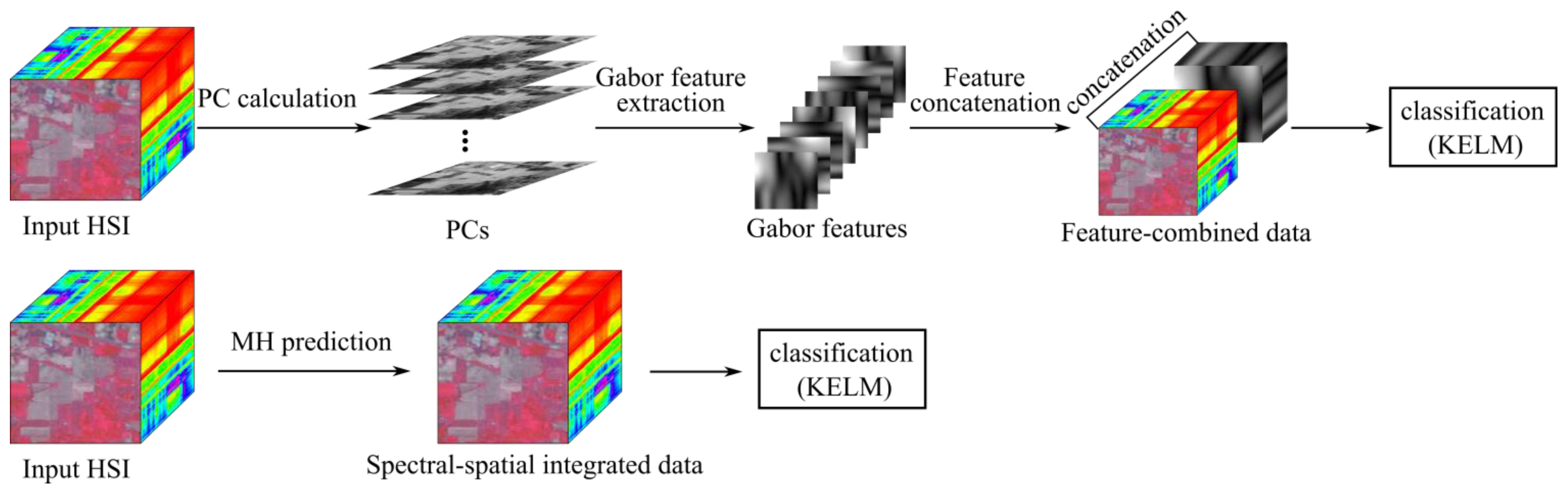
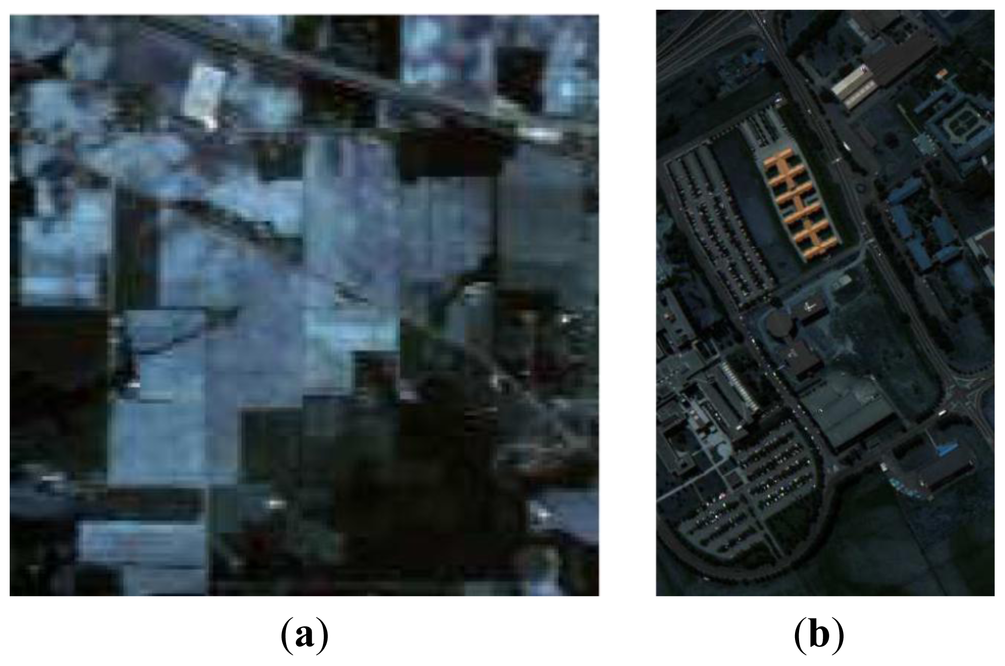
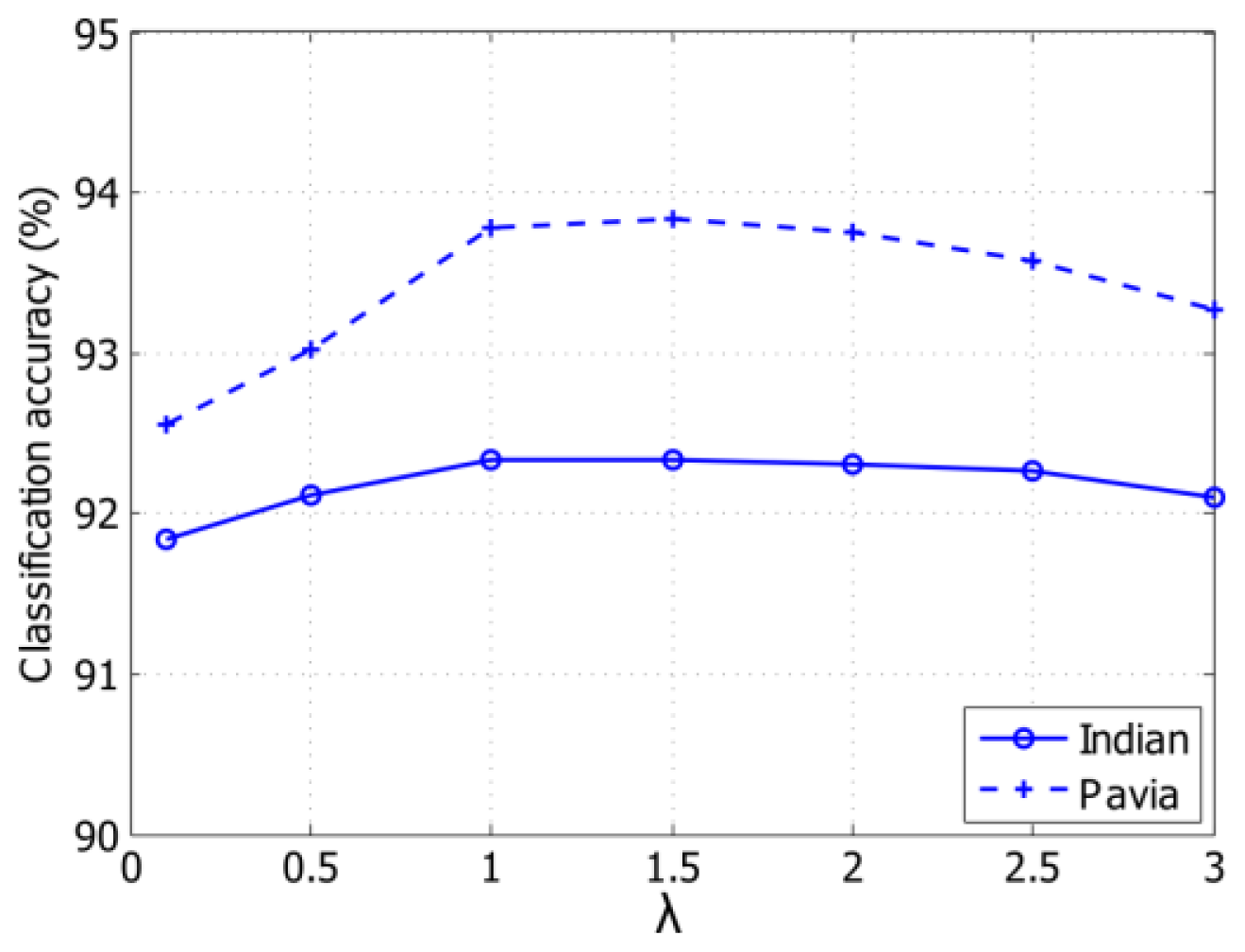
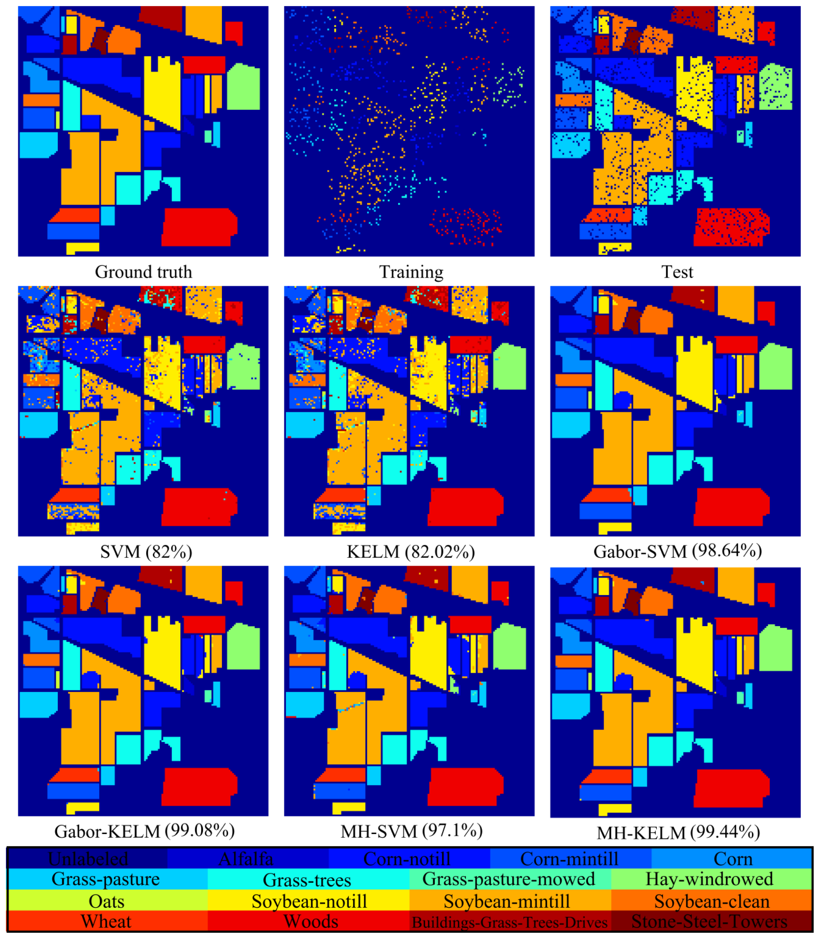
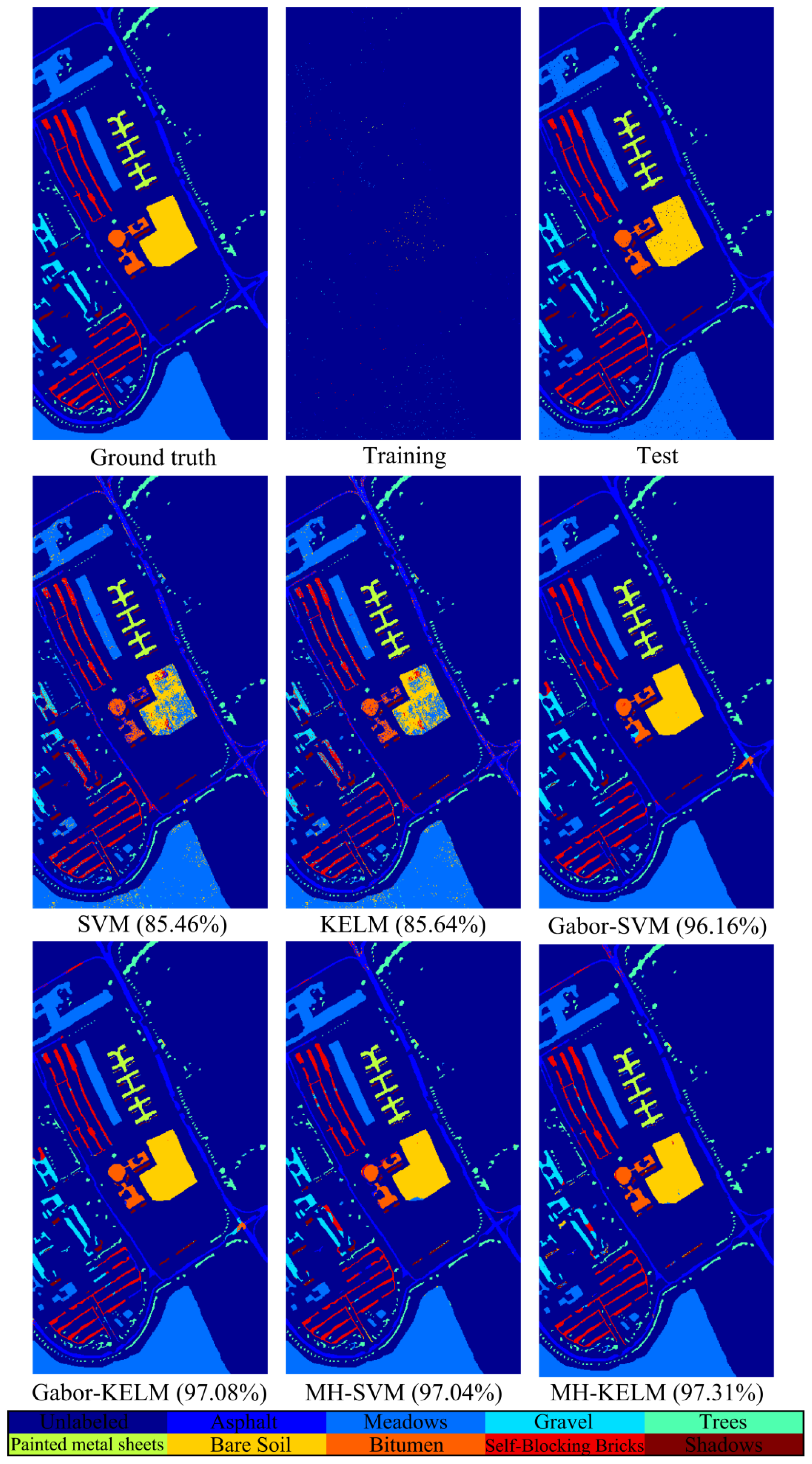
In this paper, we investigate the benefits of using spatial features (i.e., Gabor features and MH prediction) for KELM classifier under the small sample size (SSS) condition. Two real hyperspectral datasets will be employed to validate the proposed classification method. We will demonstrate that Gabor-filtering-based KELM and MH-prediction-based KELM yield superior classification performance over the conventional pixel-wise classifiers (e.g., SVM and KELM) as well as Gabor-filtering-based SVM and MH-prediction-based SVM in challenging small training sample size conditions. In addition, the proposed methods (i.e., KELM-based methods) are faster than the SVM-based methods since KELM runs at much faster learning and testing speed than the traditional SVM.
The remainder of this paper is organized as follows. Section 2 introduces the Gabor filter, MH prediction for spatial features extraction, KELM classifier, and our proposed methods. Section 3 presents the hyperspectral data and experimental setup as well as comparison of the proposed methods and some traditional techniques. Finally, Section 4 makes several concluding remarks.

2. Spectral-Spatial Kernel Extreme Learning Machine

2.1. Gabor Filter

Gabor filters are bandpass filters which have been successfully applied for a variety of image processing and machine vision applications [2326]. A 2-D Gabor function is an oriented complex sinusoidal grating modulated by a 2-D Gaussian envelope. In a 2-D coordinate (a,b) system, the Gabor filter, including a real component and imaginary one, can be represented as
G δ , θ , ψ , σ , γ ( a , b ) = exp ( - a 2 + γ 2 b 2 2 σ 2 ) × exp ( j ( 2 π a δ + ψ ) )
where
a = a cos θ + b sin θ
b = - a sin θ + b cos θ
where δ represents the wavelength of the sinusoidal factor, and θ represents the orientation separation angle of Gabor kernels (see Figure 1). Note that we need only to consider θ in the interval [0°, 180°] since symmetry makes other directions redundant. ψ is the phase offset, σ is the standard derivation of Gaussian envelope, and γ is the spatial aspects ratio (the default value is 0.5 in [27]) specifying the ellipticity of the support of the Gabor function. ψ = 0 and ψ = π/2 return the real part and imaginary part of Gabor filter, respectively. Parameter σ is determined by δ and spatial frequency bandwidth bw as
σ = δ π ln  2 2 2 bw + 1 2 bw - 1

2.2. MH Prediction for Spatial Features Extraction

In our previous work [19], a spectral-spatial preprocessing algorithm based MH prediction was proposed. It was motivated by our earlier success at applying MH prediction in compresses-sensing image and video reconstruction [28], single-image super-resolution [29], and hyperspectral image reconstruction from random projections [30]. The algorithm is driven by the idea that, for each pixel in a hyperspectral image, its neighboring pixels will likely share similar spectral characteristics or have the same class membership since HSI commonly contains homogeneous regions. Therefore, each pixel in a hyperspectral image may be represented by some linear combinations of its neighboring pixels. Specifically, multiple predictions or hypotheses drawn for a pixel of interest are made from spatially surrounding pixels. These predictions are then combined to yield a composite prediction that approximates the pixel of interest.
Consider a hyperspectral dataset with M pixels X = { X m } m = 1 M in RN (N is the dimensionality or number of spectral bands). For a pixel of interest x, the objective is to find an optimal linear combination of all possible predictions to represent x. The optimal representation can be formulated as
w ^ = argmin w x - Zw 2 2
here, Z = [z1, … zK] ∈ RN × K is a hypothesis matrix whose columns are K hypotheses generated from all neighboring pixels of x within a d × d spatial search window, and ŴRK × 1 is a vector of weighting coefficients corresponding to the K hypotheses in Z. In most cases, the dimensionality of the hypotheses is not equal to the number of hypotheses, i.e., NK, Tikhonov regularization [31] is used to regularize the least-squares problem of (5). Then, the weight vector Ŵ is calculated according to
w ^ = argmin w x - Zw 2 2 + λ x - Γ w 2 2
where Γ is the Tikhonov matrix and λ is the regularization parameter. The Γ term allows the imposition of prior knowledge on the solution. Specifically, a diagonal Γ is used in the form of
Γ = [ x - z 1 2 0 0 x - z K 2 ]
where z1, …, zK are the columns of Z. Each diagonal term in Γ measures the similarity between the pixel of interest and a hypothesis. With this structure of Γ, hypotheses which are dissimilar from the pixel of interest x are given less weights than those which are similar. The weight vector Ŵ can be calculated in a closed form
w ^ = ( Z T Z + λ Γ T Γ ) - 1 Z T x
Therefore, an approximation to x, i.e., the predicted pixel, is calculated as
x ¯ = Z w ^
For each pixel in X, a corresponding predicted pixel can be generated via (9) resulting in a predicted dataset X ¯ = { x ¯ m } m = 1 M in RN. Furthermore, once a predicted dataset is generated through MH prediction, it can be used as the current input dataset, i.e., a new X, to repeat the MH prediction process in an iterative fashion. The predicted dataset which effectively integrates spectral and spatial information is then used for classification.

2.3. Kernel Extreme Learning Machine

ELM was originally developed from feed-forward neural networks [8,32]. Recently, KELM generalizes ELM from explicit activation function to implicit mapping function, which can produce better generalization in most applications.
For C classes, let us define yk ∈ {0,1}, 1 ≤ kC. A row vector y = [y1, …, yk …, yC] indicates the class that a sample belongs to. For example, if yk = 1 and other elements in y are zero, then the sample belongs to the kth class. Given P training samples { x i , y i } i = 1 P belonging to C classes, where XiRN and yiRC, the output function of an ELM having L hidden neurons can be represented as
f ( x i ) = j = 1 L β j h ( ω j · x i + e j ) = y i ,     i = 1 , , P
where h(·) is a nonlinear activation function (e.g., Sigmoid function), βiRC is the weight vector connecting the jth hidden neuron and the output neurons, ωjRN is the weight vector connecting the j th hidden neuron and the input neurons, and ej is the bias of the jth hidden neuron. ωj · Xi denotes the inner product of ωj. and Xi. With P equations, Equation (10) can be written compactly as
H β = Y
where Y = [ y 1 T y 2 T y P T ] T R P × C , β = [ β 1 T β 2 T β L T ] T R L × C, and H is the hidden layer output matrix of the neural network:
H = [ h ( x 1 ) h ( x P ) ] = [ h ( ω 1 · x 1 + e 1 ) h ( ω L · x 1 + e L ) h ( ω 1 · x P + e 1 ) h ( ω L · x P + e L ) ] P × L
H(xi) = (h(ω1 · xi + e1), …, h(ωL · xi + eL)) is the output of the hidden neurons with respect to the input xi, which maps the data from the N-dimensional input space to the L-dimensional feature space. In most cases, the number of hidden neurons is much smaller than the number of training samples, i.e.,P, the smallest norm least-squares solution of Equation (11) proposed in [8] is defined as
β = H Y
where H is the Moore-Penrose generalized inverse of matrix H [33]. The Moore-Penrose generalized inverse of H can be calculated as H = HT (HHT)−1 [9]. For better stability and generalization, a positive value 1 ρ is added to the diagonal elements of HHT. Therefore, we have the output function of ELM classifier
f ( x i ) = h ( x i ) β = h ( x i ) H T ( I ρ + H H T ) - 1 Y
In ELM, a feature mapping h(xi) is usually known to users. If a feature mapping is unknown to users, a kernel matrix for ELM can be defined as follows:
Ω E L M = H H T : Ω E L M q , t = h ( x q ) · h ( x t ) = K ( x q , x t )
Thus, the output function of KELM can be written as
f ( x i ) = h ( x i ) H T ( I ρ + H H T ) - 1 Y = [ K ( x i , x 1 ) K ( x i , x P ) ] T ( I ρ + Ω E L M ) - 1 Y
The label of the input data is determined by the index of the output node with the largest value.

2.4. Proposed Spectral-Spatial Kernel Extreme Learning Machine

A Gabor filter can capture some physical structures of an object in an image, such as specific orientation information, using a spatial convolution kernel. Previous work [1518] has applied extracted spectral-spatial features of Gabor filter for hyperspectral image classification. Following the recent research in [17,18], a two-dimensional Gabor filter is considered to exploit the useful information in a PCA-projected subspace. The Gabor features and the original spectral features are simply concatenated. Each spatial feature (Gabor feature) vector and spectral feature vector are normalized to have a unit l2 norm before feature concatenation or stacking. We note that the implementation of Gabor filter in a subset of original bands with band selection [34] could equally be employed. The Gabor-filtering-based KELM is denoted as Gabor-KELM. We also employ the MH prediction as the preprocessing of KELM classifier, which is denoted as MH-KELM. The proposed spectral-spatial KELM framework is illustrated in Figure 2.

3. Experiments

In this section, we compare the classification performance of proposed Gabor-KELM and MH-KELM with SVM, KELM, Gabor-filtering-based SVM (Gabor-SVM), and MH-prediction-based SVM (MH-SVM). SVM with radial basis function (RBF) kernel is implemented using the libsvm package [35]. For KELM with RBF kernel, we use the implementation available from the ELM website [36].

3.1. Data Description and Experimental Setup

We validate the effectiveness of proposed methods, i.e., Gabor-KELM and MH-KELM, using two hyperspectral datasets. The first HSI dataset in our tests was acquired using NASA’s Airborne Visible/Infrared Imaging Spectrometer (AVIRIS) sensor and was collected over northwest Indiana’s Indian Pines test site in June 1992. This scene represents a vegetation-classification scenario with 145 × 145 pixels in the 0.4–2.45-μm region of the visible and infrared spectrum with a spatial resolution of 20 m. For this dataset, spectral bands {104–108, 150–163, 220} correspond to water-absorption bands are removed, resulting in 200 spectral bands. The original Indian Pines dataset consists of 16 ground-truth land-cover classes.
The second dataset used in our experiments, University of Pavia, is an urban scene acquired by the Reflective Optics System Imaging Spectrometer (ROSIS) [37]. The image scene, covering the city of Pavia, Italy, was collected under the HySens project managed by DLR (the German Aerospace Agency) [38]. The ROSIS sensor generates 115 spectral bands ranging from 0.43 to 0.86 μm and has a spatial resolution of 1.3 m per pixel and contains 610 × 340 pixels. The dataset consists of 103 spectral bands with the 12 noisiest bands removed. The labeled ground truth of this dataset is comprised of 9 classes. The class descriptions and sample distributions for both the Indian Pines and University of Pavia datasets are given in Table 1 and 2. Both datasets, and their corresponding ground truth maps, are obtained from the publicly available website [39] of the Computational Intelligence Group from the Basque University (UPV/EHU). False-color images of two datasets are displayed in Figure 3.
For the Indian Pines dataset, some of the classes contain a small number of samples. For example, the Oats class has only 20 samples. In one of our experiments, we sort the 16 classes according to the number of samples in each class in ascending order and conduct a separate set of experiments with the last nine classes, allowing for more training samples from a statistical viewpoint [5]. The class numbers of the nine classes are highlighted in boldface in Table 1. The SSS condition will be discussed in the following work, and if we select 20 labeled samples per class (180 total), all the left will be ones to be classified. Each classification experiment is repeated for 10 trials with different training and testing samples, and overall classification accuracy is averaged over 10 repeated trials. The University of Pavia dataset is processed similarly, the only difference being that we first choose 900 samples at random from each class to form the total sample set (8100 total) for each trial. Then, the training and testing samples are chosen randomly from each class of the total sample set for classification. This procedure is used since some classes of the University of Pavia dataset contain significantly more samples than other classes, which might bias the accuracy. In order to have a fair comparison, the number of samples per class should be equal or similar.
All experiments are carried out using MATLAB (except SVM, which is implemented in C) on an Intel i7 Quadcore 2.63-GHz machine with 6 GB of RAM.

3.2. Parameter Tuning

First of all, we study the parameters of Gabor filter for hyperspectral images. In our work, eight orientations, [ 0 , π 8 , π 4 , 3 π 8 , π 2 , 5 π 8 , 3 π 4 , 7 π 8 , ], as shown in Figure 1 are considered. According to Equation (4), δ and bw are the two parameters of Gabor filter to be investigated. We test different δ and bw as shown in Figure 4a for the Indian Pines dataset and (b) for the University of Pavia dataset. Figure 4 illustrates the classification accuracy of the proposed Gabor-KELM versus varying δ as well as bw. Note that for Gabor-KELM in the experiment, we empirically choose the first 10 principal components (PCs) of both datasets that account for over 99% of the total variation in the images. From the results, we set the optimal δ and bw for both experimental datasets to 26 and 1, respectively.
An important parameter involved in MH prediction is the search-window size d used in hypothesis generation. We analyze the effect of the search-window size in terms of the overall classification accuracy as well as the execution time of the algorithm. A set of window sizes, d ∈ {3, 5, 7, 9, 11, 13}, is used for testing. From Figure 5, we can see that the classification accuracies are similar when the window size is between 9 × 9 and 13 × 13. We also find that using d = 11 takes over twice the execution time of d = 9 but does not yield any significant gains in classification accuracy. Specifically, Table 3 shows the execution time of one iteration of MH prediction for various search-window sizes. In all the experiments, two iterations of MH prediction are used. Another important parameter is λ that controls the relative effect of the Tikhonov regularization term in the optimization of Equation (6). Many approaches have been presented in the literature—such as L-curve [40], discrepancy principle, and generalized cross-validation (GCV)—for finding an optimal value for such regularization parameter. Here, we find an optimal λ by examining a set of values as shown in Figure 6, which presents the overall classification accuracy with different values of λ for MH prediction. One can see that the classification accuracy is quite stable over the interval λ ∈ [1, 2]. As a result, in all the experiments reported here, we use λ = 1.5.

3.3. Classification Results

The SSS problem is one of the most fundamental and challenging issues in hyperspectral image classification. In practice, the number of available labeled samples is often insufficient for hyperspectral images. Thus, we investigate the classification accuracy of aforementioned classifiers as a function of different labeled samples size, varying from 20–40 per class. To avoid any bias, all the experiments are repeated 10 times, and we report the averaged classification accuracy as well as the corresponding standard deviation. In all experiments, if no specific instructions, the tuning parameters of KELM (RBF kernel parameters) and the parameters of the competing method (SVM) are chosen as those that maximize the training accuracy by means of five-fold cross-validation to avoid over-fitting. The performance of the proposed spectral-spatial-based KELM methods is shown in Tables 4 and 5 for two experimental data.
From the results of each individual classifier, with Gabor features or MH prediction, the classification accuracy is significantly improved at all training sample sizes compared with the accuracy of classifying with the original spectral signature only. For example, in Table 4, Gabor-SVM has 26.9% higher accuracy than SVM, MH-SVM has 21.8% higher accuracy than SVM, Gabor-KELM has 24.7% higher accuracy than KELM, and MH-KELM has 24.1% higher accuracy than KELM when there are 20 labeled samples per class for training for the Indian Pines dataset. Moreover, for the Indian Pines dataset, KELM employing spatial features (Gabor features or MH prediction) achieved better classification performance than SVM employing spatial features. Especially for the MH-prediction-based methods, the accuracy of proposed MH-KELM is always about 5% higher than MH-SVM at all sample sizes. For the University of Pavia dataset, in terms of classification accuracy, Gabor-KELM outperforms Gabor-SVM, and MH-KELM outperforms MH-SVM. It is interesting to notice that the performance of Gabor-KELM is close to MH-KELM for both datasets, which demonstrates that KELM has better generalization than SVM.
Based on the results shown in Tables 4 and 5, we further perform the standard McNemar’s test [41], which is based on a standardized normal test statistic
Z = f 12 - f 21 f 12 + f 21
where f12 indicates the number of samples classified correctly by classifier 1 and simultaneously misclassified by classifier 2. The test is employed to verify the statistical significance in accuracy improvement of the proposed method. Tables 6 and 7 present the statistical significance from the standardized McNemar’s test about the difference between the proposed KELM-based methods and the traditional SVM-based methods. In these two tables, classifier 1 is denoted as C1 and classifier 2 is denoted as C2. As listed in the tables, the difference in accuracy between the two methods is viewed to be significantly differently at 95% confidence level if |Z| > 1.96 and at 99% confidence level if |Z| > 2.58. Moreover, the sign of Z indicates whether classifier 1 outperforms classifier 2 (Z > 0) or vice versa. We can observe that the overall results of McNemar’s test for both datasets all have negative signs. This demonstrates that KELM-based methods outperform SVM-based methods, which confirms the conclusions obtained from the classification accuracies as shown in Tables 4 and 5.
We also conduct an experiment using the whole scene of the two datasets. For the Indian Pines dataset, we randomly select 10% of the samples from each class (16 classes are used in this experiment) for training and the rest for testing. For the University of Pavia dataset, we use 1% of the samples from each class for training and the rest for testing. The classification accuracy for each class, overall accuracy (OA), average accuracy (AA), and the Cohen-κ are shown in Tables 8 and 9 for the two datasets, respectively. As can be seen from Tables 8 and 9, the proposed Gabor-KELM and MH-KELM have superior performance to the pixel-wise classifiers and outperform Gabor-SVM and MH-SVM. More importantly, we can see that employing the spatial features for classification can improve the accuracy under the SSS condition. For example, in Table 8, the classification accuracies for class 1 (four training samples), 7 (two training samples) and 9 (two training samples) improved over 40% by integrating the spatial information (i.e., Gabor features or MH prediction) for KELM classifier. Due to the high cost of training data, such performance at low numbers of training data is important in many applications. Hence, we conclude that proposed Gabor-KELM and MH-KELM are very effective classification strategies for hyperspectral data analysis tasks under the SSS condition. Figures 7 and 8 provide a visual inspection of the classification maps generated using the whole HSI scene for the Indian Pines dataset (145 × 145 including unlabeled pixels) and the University of Pavia dataset (610 × 340, including unlabeled pixels), respectively. As shown in the two figures, classification maps of spectral-spatial based classification methods are less noisy and more accurate than maps generated from pixel-wise classification methods. Moreover, spectral-spatial based classification methods exhibit better spatial homogeneity than pixel-wise classification methods. This homogeneity is observable within almost every labeled area.
Finally, we report the computational complexity of the aforementioned classification methods using 20 labeled samples per class. All experiments are carried out using MATLAB on an Intel i7 Quadcore 2.63-GHz machine with 6 GB of RAM. The execution time for the two experimental data is listed in Table 10. For spectral-spatial based methods, we report the time for feature extraction and classification (training and testing) separately. It should be noted that SVM is implemented in the libsvm package which uses the MEX function to call C program in MATLAB while KELM is implemented purely in MATLAB. As can be seen in Table 10, in terms of execution time of pixel-wise classifiers, KELM is much faster than SVM even though SVM is implemented in C. For the spectral-spatial based classifiers (i.e., Gabor-filtering-based and MH-prediction-based classifiers) are, as expected, much slower than the pixel-wise classifiers due to the fact that they carry the additional burden of spatial feature extraction (i.e., Gabor filtering on PCs, or MH prediction preprocessing). MH-prediction-based methods are the most time-consuming ones since two iterations of MH prediction are used in the experiments and the weight vector Ŵ has to be calculated for every pixel in the image according to Equation (8) during MH prediction. It is worth mentioning that Gabor feature extraction procedure is performed independently on each PC, which means that Gabor feature extraction can go parallel. Thus, the speed of Gabor feature extraction on PCs can be greatly improved.

4. Conclusions

In this paper, we proposed to integrate spectral and spatial information to improve the performance of KELM classifier by using Gabor features and MH prediction preprocessing. Specifically, a simple two-dimensional Gabor filter was implemented to extract spatial features in the PCA-projected domain. MH prediction preprocessing makes use of the spatial piecewise-continuous nature of hyperspectral imagery to integrate spectral and spatial information. The proposed classification techniques, i.e., Gabor-KELM and MH-KELM, have been compared with the conventional pixel-wise classifiers, such as SVM and KELM, as well as Gabor-SVM and MH-SVM, under the SSS condition for hyperspectral data. Experimental results have demonstrated that the proposed methods can outperform the conventional pixel-wise classifiers as well as Gabor-filtering-based SVM and MH-prediction-based SVM in challenging small training sample size conditions. Specifically, the proposed spectral-spatial classification methods achieved over 16% and 9% classification accuracy improvement over the pixel-wise classification methods for the Indian Pines dataset and the University of Pavia dataset, respectively. MH-KELM outperformed MH-SVM by about 5% for the Indian Pines dataset and Gabor-KELM outperformed Gabor-SVM by about 1.3% for the University of Pavia dataset at all training sample sizes. Moreover, KELM exhibits very fast training and testing speed, which is an important attribute for hyperspectral analysis applications. Although the proposed methods carry additional burden on spatial feature extraction, the computational cost can be reduced by parallel computing.

Acknowledgments

This research was supported in part by National Natural Science Foundation of China (41201341, 61302164), Key Laboratory of Satellite Mapping Technology and Application, National Administration of Surveying, Mapping and Geoinformation (KLSMTA-201301), and Key Laboratory of Advanced Engineering Surveying of National Administration of Surveying, Mapping and Geoinformation (No. TJES1301).

Conflicts of Interest

The authors declare no conflict of interest.
  • Author ContributionsAll authors conceived and designed the study. Chen Chen and Wei Li carried out the experiments. All authors discussed the basic structure of the manuscript, and Chen Chen finished the first draft. Wei Li, Hongjun Su and Kui Liu reviewed and edited the draft.

References

  1. Harsanyi, J.C.; Chang, C.-I. Hyperspectral image classification and dimensionality reduction: An orthogonal subspace projection approach. IEEE Trans. Geosci. Remote Sens 1994, 32, 779–785. [Google Scholar]
  2. Ratle, F.; Camps-Valls, G.; Weston, J. Semisupervised neural networks for efficient hyperspectral image classification. IEEE Trans. Geosci. Remote Sens 2010, 48, 2271–2282. [Google Scholar]
  3. Plaza, J.; Plaza, A.; Perez, R.; Martinez, P. Parallel Classification of Hyperspectral Images Using Neural Networks. In Computational Intelligence for Remote Sensing; Grana, M., Duro, R.J., Eds.; Springer-Verlag: Berlin, Germany, 2008; Volume 133, pp. 193–216. [Google Scholar]
  4. Bazi, Y.; Melgani, F. Toward an optimal SVM classification system for hyperspectral remote sensing images. IEEE Trans. Geosci. Remote Sens 2006, 44, 3374–3385. [Google Scholar]
  5. Melgani, F.; Bruzzone, L. Classification of hyperspectral remote sensing images with support vector machines. IEEE Trans. Geosci. Remote Sens 2004, 42, 1778–1790. [Google Scholar]
  6. Landgrebe, D.A. Signal Theory Methods in Multispectral Remote Sensing; Wiley-Interscience: Hoboken, NJ, USA, 2003. [Google Scholar]
  7. Foody, G.M.; Ajay, M. A relative evaluation of multiclass image classification by support vector machines. IEEE Trans. Geosci. Remote Sens 2004, 42, 1335–1343. [Google Scholar]
  8. Huang, G.-B.; Zhu, Q.-Y.; Siew, C.-K. Extreme learning machine: Theory and applications. Neurocomputing 2006, 70, 489–501. [Google Scholar]
  9. Huang, G.-B.; Zhou, H.; Ding, X.; Zhang, R. Extreme learning machine for regression and multiclass classification. IEEE Trans. Syst. Man Cybern. Part. B 2012, 42, 513–529. [Google Scholar]
  10. Moreno, R.; Corona, F.; Lendasse, A.; Grana, M.; Galvao, L.S. Extreme learning machine for soybean classification in remote sensing hyperspectral images. Neurocomputing 2014, 128, 207–216. [Google Scholar]
  11. Pal, M. Extreme-learning-machine-based land cover classification. Int. J. Remote Sens 2009, 30, 3835–3841. [Google Scholar]
  12. Pal, M.; Maxwell, A.E.; Warner, T.A. Kernel-based extreme learning machine for remote-sensing image classification. Remote Sens. Lett 2013, 4, 853–862. [Google Scholar]
  13. Camps-Valls, G.; Gomez-Chova, L.; Munoz-Mari, J.; Vila-Frances, J.; Calpe-Maravilla, J. Composite kernels for hyperspectral image classification. IEEE Geosci. Remote Sens. Lett 2006, 3, 93–97. [Google Scholar]
  14. Huang, X.; Zhang, L. An SVM ensemble approach combining spectral, structural, and semantic features for the classification of high-resolution remotely sensed imagery. IEEE Trans. Geosci. Remote Sens 2013, 51, 257–272. [Google Scholar]
  15. Bau, T.C.; Sarkar, S.; Healey, G. Hyperspectral region classification using a three-dimensional Gabor filterbank. IEEE Trans. Geosci. Remote Sens 2010, 48, 3457–3464. [Google Scholar]
  16. Shen, L.; Jia, S. Three-dimensional Gabor wavelets for pixel-based hyperspectral imagery classification. IEEE Trans. Geosci. Remote Sens 2011, 49, 5039–5046. [Google Scholar]
  17. Huo, L.-Z.; Tang, P. Spectral and Spatial Classification of Hyperspectral Data Using SVMs and Gabor Textures. Proceedings of IEEE International Geoscience and Remote Sensing Symposium, Vancouver, BC, Canada, 24–29 July 2011; pp. 1708–1711.
  18. Zhang, L.; Zhang, L.; Tao, D.; Huang, X. On combining multiple features for hyperspectral remote sensing image classification. IEEE Trans. Geosci. Remote Sens 2012, 50, 879–893. [Google Scholar]
  19. Chen, C.; Li, W.; Tramel, E.W.; Cui, M.; Prasad, S.; Fowler, J.E. Spectral-spatial preprocessing using multihypothesis prediction for noise-robust hyperspectral image classification. IEEE J. Sel. Top. Appl. Earth Observ. Remote Sens 2014, 7, 1047–1059. [Google Scholar]
  20. Huang, X.; Zhang, L. An adaptive mean-shift analysis approach for object extraction and classification from urban hyperspectral imagery. IEEE Trans. Geosci. Remote Sens 2008, 46, 4173–4185. [Google Scholar]
  21. Kettig, R.L.; Landgrebe, D.A. Classification of multispectral image data by extraction and classification of homogeneous objects. IEEE Trans. Geosci. Electron 1976, GE-14, 19–26. [Google Scholar]
  22. Landgrebe, D.A. The development of a spectral-spatial classifier for earth observational data. Pattern Recognit 1980, 12, 165–175. [Google Scholar]
  23. Huang, L.L.; Shimizu, A.; Kobatake, H. Robust face detection using Gabor filter features. Pattern Recognit. Lett 2005, 26, 1641–1649. [Google Scholar]
  24. Jain, A.K.; Ratha, N.K.; Lakshmanan, S. Object detection using gabor filters. Pattern Recognit 1997, 30, 295–309. [Google Scholar]
  25. Porat, M.; Zeevi, Y.Y. The generalized Gabor scheme of image representation in biological and machine vision. IEEE Trans. Pattern Anal. Mach. Intell 1988, 10, 452–468. [Google Scholar]
  26. Hamamoto, Y.; Uchimura, S.; Watanabe, M.; Yasuda, T.; Mitani, Y.; Tomita, S. Object A gabor filter-based method for recognizing handwritten numerals. Pattern Recognit 1998, 31, 395–400. [Google Scholar]
  27. Clausi, D.A.; Jernigan, M.E. Designing Gabor filters for optimal texture separabilty. Pattern Recognit 2000, 33, 1835–1849. [Google Scholar]
  28. Chen, C.; Tramel, E.W.; Fowler, J.E. Compressed-Sensing Recovery of Images and Video Using Multihypothesis Predictions. Proceedings of the 2011 Asilomar Conference on Signals, Systems, and Computers, Pacific Grove, CA, USA, 6–9 November 2011; pp. 1193–1198.
  29. Chen, C.; Fowler, J.E. Single-Image Super-Resolution Using Multihypothesis Prediction. Proceedings of the 2012 Asilomar Conference on Signals, Systems, and Computers, Pacific Grove, CA, USA, 4–7 November 2012; pp. 1193–1198.
  30. Chen, C.; Li, W.; Tramel, E.W.; Fowler, J.E. Reconstruction of hyperspectral imagery from random projections using multihypothesis prediction. IEEE Trans. Geosci. Remote Sens 2014, 52, 365–374. [Google Scholar]
  31. Tikhonov, A.N.; Arsenin, V.Y. Solutions of Ill Posed Problems; Winston & Sons: Washington, DC, USA, 1977. [Google Scholar]
  32. Huang, G.-B.; Chen, L.; Siew, C.-K. Universal approximation using incremental constructive feedforward networks with random hidden nodes. IEEE Trans. Neural Netw 2006, 17, 879–892. [Google Scholar]
  33. Serre, D. Matrices: Theory and Applications; Springer-Verlag: New York, NY, USA, 2002. [Google Scholar]
  34. Du, Q.; Yang, H. Similarity-based unsupervised band selection for hyperspectral image analysis. IEEE Geosci. Remote Sens. Lett 2008, 5, 564–568. [Google Scholar]
  35. LIBSVM—A Library for Support Vector Machines. Available online: http://www.csie.ntu.edu.tw/~cjlin/libsvm (accessed on 5 March 2014).
  36. MATLAB Codes for Extreme Learning Machine (ELM) Algorithm. Available online: http://www.ntu.edu.sg/home/egbhuang/elm_kernel.html (accessed on 7 March 2014).
  37. Gamba, P. A Collection of Data for Urban Area Characterization. Proceedings of 2004 IEEE International Geoscience and Remote Sensing Symposium, Anchorage, AK, USA, 20–24 September 2004; pp. 69–72.
  38. Huang, X.; Zhang, L. A comparative study of spatial approaches for urban mapping using hyperspectral ROSIS images over Pavia City northern Italy. Int. J. Remote Sens 2009, 30, 3205–3221. [Google Scholar]
  39. Hyperspectral Remote Sensing Scenes. Available online: http://www.ehu.es/ccwintco/index.php/Hyperspectral_Remote_Sensing_Scenes (accessed on 20 December 2013).
  40. Hansen, C.; O’Leary, D.P. The use of the L-curve in the regularization of discrete ill-posed problems. SIAM J. Sci. Comput 1993, 14, 1487–1503. [Google Scholar]
  41. Villa, A.; Benediktsson, J.A.; Chanussot, J.; Jutten, C. Hyperspectral image classification with independent component discriminant analysis. IEEE Trans. Geosci. Remote Sens 2011, 49, 4865–4876. [Google Scholar]
Figure 1. Two-dimensional Gabor kernels with different orientations, from left to right: 0, π/8, π/4, 3π/8, π/2, 5π/8, 3π/4, and 7π/8.
Remotesensing 06 05795f1
Figure 2. The proposed spectral-spatial KELM framework for hyperspectral image classification (first row: Gabor-KELM; second row: MH-KELM).
Remotesensing 06 05795f2
Figure 3. False-color images: (a) Indian Pines dataset, using bands 10, 20, and 30 for red, green, and blue, respectively; and (b) University of Pavia dataset, using bands 20, 40, and 60 for red, green, and blue, respectively.
Remotesensing 06 05795f3
Figure 4. Classification accuracy (%) versus varying δ and bw for the proposed Gabor-KELM using 20 labeled samples per class for (a) Indian Pines dataset; and (b) University of Pavia dataset.
Remotesensing 06 05795f4
Figure 5. Classification accuracy (%) versus varying search-window size (d) for the proposed MH-KELM using 20 labeled samples per class for two experimental datasets.
Remotesensing 06 05795f5
Figure 6. Classification accuracy (%) for Indian Pines and University of Pavia datasets as a function of the MH-prediction regularization parameter λ for the proposed MH-KELM using 20 labeled samples per class. The search-window size for MH prediction is d = 9 × 9.
Remotesensing 06 05795f6
Figure 7. Thematic maps resulting from classification using 1018 training samples (10% per class) for the Indian Pines dataset with 16 classes. The overall classification accuracy of each algorithm is indicated in parentheses.
Remotesensing 06 05795f7
Figure 8. Thematic maps resulting from classification using 423 training samples (1% per class) for the University of Pavia dataset. The overall classification accuracy of each algorithm is indicated in parentheses.
Remotesensing 06 05795f8
Table 1. Per-class samples for the Indian Pines dataset.
ClassNumber of Samples

No.Name
1Alfalfa46
2Corn-notill1428
3Corn-mintill830
4Corn237
5Grass-pasture483
6Grass-trees730
7Grass-pasture-mowed28
8Hay-windrowed478
9Oats20
10Soybean-notill972
11Soybean-mintill2455
12Soybean-clean593
13Wheat205
14Woods1265
15Building-grass-trees-drives386
16Stone-steel-towers93

Total10,249
Table 2. Per-class samples for the University of Pavia dataset.
ClassNumber of Samples

No.Name
1Asphalt6631
2Meadows18,649
3Gravel2099
4Trees3064
5Painted metal sheets1345
6Bare soil5029
7Bitumen1330
8Self-blocking bricks3682
9Shadows947

Total42,776
Table 3. Execution time (s) for one iteration of MH prediction for the Indian Pines dataset as a function of search-window size d.
Window Size (d)Time (s)
36.4
513.7
739.4
9109.5
11260.2
13564.6
Table 4. Overall classification accuracy (%)—mean ± standard deviation over 10 trials using varying number of labeled training samples (ratio represents the proportion of labeled training samples and samples to be classified) per class for the Indian Pines dataset (nine classes).
MethodNumber of Training Samples Per Class (Ratio)

20 (1.99%)30 (3.01%)40 (4.06%)
SVM65.83 ± 2.7171.96 ± 2.2075.67 ± 1.39
KELM68.28 ± 2.0472.97 ± 1.4776.02 ± 1.45

Gabor-SVM92.74 ± 1.2295.25 ± 1.2696.51 ± 1.05
Gabor-KELM93.02 ± 1.0895.44 ± 1.0396.64 ± 1.14

MH-SVM87.61 ± 2.0189.91 ± 1.0591.87 ± 0.86
MH-KELM92.43 ± 1.8994.87 ± 0.9896.75 ± 0.78
Table 5. Overall classification accuracy (%)—mean ± standard deviation over 10 trials using a varying number of labeled training samples (ratio represents the proportion of labeled training samples and samples to be classified) per class for the University of Pavia dataset.
MethodNumber of Training Samples Per Class (Ratio)

20 (2.27%)30 (3.45%)40 (4.65%)
SVM81.11 ± 1.1582.80 ± 0.8684.09 ± 0.63
KELM81.21 ± 1.6482.96 ± 0.9884.34 ± 0.64

Gabor-SVM90.83 ± 1.1193.45 ± 1.4894.88 ± 0.85
Gabor-KELM92.57 ± 1.4994.77 ± 1.2696.07 ± 0.92

MH-SVM92.85 ± 0.9194.89 ± 0.7495.74 ± 0.47
MH-KELM93.14 ± 1.0595.29 ± 0.6896.31 ± 0.53
Table 6. McNemar’s test (Z ) for the Indian Pines dataset (nine classes, 20 samples per class for training).
Class(SVM, KELM)(C1, C2)(Gabor-SVM, Gabor-KELM)(C1, C2)(MH-SVM, MH-KELM)(C1, C2)
Hay-windrowed1.73NaNNaN
Grass-pasture−0.262.832.00
Soybean-clean0.321.514.56
Grass-trees−0.76−1.41−0.77
Corn-mintill2.565.404.06
Soybean-notill1.532.896.35
Woods2.45−1.73−0.20
Corn-notill3.514.678.09
Soybean-mintill8.30−7.0012.23
Overall6.091.3416.65
Table 7. McNemar’s test (Z) for the University of Pavia dataset (180 training and 7920 testing samples).
Class(SVM, KELM)(C1, C2)(Gabor-SVM, Gabor-KELM)(C1, C2)(MH-SVM, MH-KELM) (C1, C2)
Asphalt7.01−1.294.51
Meadows−4.824.56−6.29
Gravel0−6.400.54
Trees−2.47−1.132.71
Painted metal sheets−1.73−1.00−1.00
Bare Soil−1.07−7.75−0.23
Bitumen−2.72−5.66−3.15
Self-Blocking Bricks−2.10−0.99−5.17
Shadows5.66−1.046.71
Overall−0.50−6.29−0.97
Table 8. Classification accuracy (%) for the Indian Pines dataset (16 classes).
ClassSamplesSVMKELMGabor-SVMGabor-KELMMH-SVMMH-KELM

TrainTest
Alfalfa44257.1454.7664.2997.6226.1990.48
Corn-notill142128678.8581.0398.7698.6897.4398.99
Corn-mintill8374762.2562.7897.8698.3996.1299.06
Corn2321450.0053.7498.1399.0796.2699.53
Grass-pasture4843593.5690.8099.5410097.47100
Grass-trees7365795.2895.2810010099.70100
Grass-pasture-mowed226042.31092.31096.15
Hay-windrowed4743196.2998.8410010099.30100
Oats218033.331001000100
Soybean-notill9787569.9471.6699.3198.1796.9199.89
Soybean-mintill245221088.6485.4899.3299.2897.2499.41
Soybean-clean5953476.9772.6697.7597.5798.8898.50
Wheat2018599.4698.9296.6298.92100100
Woods126113997.5495.6110010099.91100
Bldg-Grass-Trees-Drives3834844.5462.9397.9998.8597.7099.14
Stone-Steel-Towers98494.0575.0010010095.2498.81
OA82.0082.0298.6499.0897.1099.44
AA69.0373.4590.5798.6881.1598.75
κ79.2879.3798.4498.9596.6999.36
Table 9. Classification accuracy (%) for the University of Pavia dataset (whole scene).
ClassSamplesSVMKELMGabor-SVMGabor-KELMMH-SVMMH-KELM

TrainTest
Asphalt66656587.0284.0194.3094.4997.9396.29
Meadows1861846397.2897.5199.8299.9699.9199.98
Gravel20207957.5861.2893.2795.0087.0193.25
Trees30303474.0376.4394.9995.4594.9696.30
Painted metal sheets13133299.2599.4799.7799.9299.5599.70
Bare Soil50497957.0260.8899.9299.9898.5799.46
Bitumen13131763.6372.5988.2398.5682.3895.67
Self-Blocking Bricks36364686.4883.1985.2488.6294.3097.11
Shadows993898.8386.9975.6979.6482.7352.35
OA993885.4685.496.1697.0897.0497.31
AA80.1280.2692.3694.6293.0492.23
κ80.2380.5394.8996.1296.0696.42
Table 10. Execution time for the Indian Pines dataset (nine classes, 180 training and 9054 testing samples) and the University of Pavia dataset (180 training and 7920 testing samples).
MethodIndian PinesUniversity of Pavia

Time (s)(Feature Extraction)Time (s)(Classification)Time (s)(Feature Extraction)Time (s)(Classification)
SVM-0.94-0.89
KELM-0.23-0.17
Gabor-SVM46.831.02377.040.93
Gabor-KELM46.830.27377.040.20
MH-SVM215.400.91479.780.85
MH-KELM215.400.25479.780.16

