A Python-Based Open Source System for Geographic Object-Based Image Analysis (GEOBIA) Utilizing Raster Attribute Tables

Abstract

A modular system for performing Geographic Object-Based Image Analysis (GEOBIA), using entirely open source (General Public License compatible) software, is presented based around representing objects as raster clumps and storing attributes as a raster attribute table (RAT). The system utilizes a number of libraries, developed by the authors: The Remote Sensing and GIS Library (RSGISLib), the Raster I/O Simplification (RIOS) Python Library, the KEA image format and TuiView image viewer. All libraries are accessed through Python, providing a common interface on which to build processing chains. Three examples are presented, to demonstrate the capabilities of the system: (1) classification of mangrove extent and change in French Guiana; (2) a generic scheme for the classification of the UN-FAO land cover classification system (LCCS) and their subsequent translation to habitat categories; and (3) a national-scale segmentation for Australia. The system presented provides similar functionality to existing GEOBIA packages, but is more flexible, due to its modular environment, capable of handling complex classification processes and applying them to larger datasets.

1. Introduction

The advantages of Geographic Object-Based Image Analysis (GEOBIA) over more traditional pixel-based analyses have been discussed in a number of studies [1–4]. Whilst a large body of the literature has utilized commercial packages, such as eCognition [5], there is growing interest in open source alternatives [6]. This is part of a wider interest in open source software within the geospatial field [7]. The benefits of open source software go beyond cost savings on software licenses. For researchers, open source software provides the ability to interrogate existing algorithms, by looking at the source code, and to adapt them as required [8]. Open source software can also provide access to the latest algorithms [9]. With the popularity of publicly accessible version control systems (e.g., GitHub, Bitbucket, SourceForge and Google Code) for managing open source projects, the latest algorithms are often available before being published for those users willing to use a development version of the software.

With the increasing availability of datasets, at higher temporal and spatial resolutions (e.g., ESA Sentinel’s), there is a greater need for software that is capable of efficiently handling large volumes of data, preferably in as automated a way as possible. Alongside the increase in data volume, the computing resources to process data have dramatically increased. Through high performance computing (HPC) facilities and cloud computing platforms (e.g., Amazon EC2, Microsoft Azure), more computing power is available to perform GEOBIA, which often requires more resources than traditional pixel-based techniques. However, the effective use of these resources requires software capable of scaling to a large number of nodes in a manner that is computationally efficient and cost effective.

There are currently a number of open source packages that can be used to perform various parts of the GEOBIA process. For example, the Orfeo Toolbox (OTB; [10]) from the French Centre National d'Études Spatiales (CNES) provides a number of algorithms for image segmentation and feature extraction and is built on top of the Insight Segmentation and Registration Toolkit (ITK; http://www.itk.org/), which contains a number of segmentation algorithms in use by the medical community. Within OTB, there are also per-pixel methods for image classification, including a number of machine learning algorithms through OpenCV ( http://opencv.org). The TWinned Object and Pixel-based Automated classification Chain (TWOPAC; [11]) aims to be a complete framework for pixel and object-based classification utilizing a decision tree approach for classification. However, the authors currently perform the segmentation outside of the framework using eCognition. InterIMAGE is an open source package with similar functions to eCognition; it provides a GUI through which a series of processing steps (e.g., segmentation and classification) and decision rules can be programmed as a semantic net and executed [12]. However, InterImage is currently limited in the volume of data it can process within a single project, with a maximum scene size of 3000 × 3000 pixels [12].

Given the advantages of GEOBIA and the desirability of open source software, this paper presents a complete open source framework for performing GEOBIA using a number of open source libraries, developed by the authors. All libraries are accessed through Python, providing a common interface on which processing chains can be built. This paper provides a description of the individual libraries and how they are combined to provide GEOBIA functionality. The system is compared to existing GEOBIA systems and three examples of published and ongoing research are presented, which provide insight into the capabilities offered. Finally, adding existing external packages to the modular system is discussed along with plans for future work.

2. Software Libraries

The open source GEOBIA system presented is built around representing objects as raster clumps (groups of pixels, the values of which provide the ID) and storing the attributes of each object (clump) within a raster attribute table (RAT), linked by the clump ID (Figure 1).

To create, store, visualize and classify the objects within the RAT, the following packages are used:

• GDAL; raster data model and input and output (I/O) of common image formats.
• RSGISLib; segmentation and attribution of objects.
• Raster I/O Simplification (RIOS); used to read, write and classify attributed objects.
• TuiView; used to view data and provides a GUI for rule development.
• KEA Image format; used to store image objects and associated attributes.

With the exception of RSGISLib, which is currently only tested under UNIX and UNIX-like operating systems (e.g., Linux, OS X, Solaris), all of the software is fully cross platform and will work under Linux, OS X or Windows.

2.1. GDAL

The Geospatial Data Abstraction Library (GDAL; www.gdal.org) provides a generic library through which all of the common image file formats used within the field of remote sensing data can be accessed. The GDAL data model is based on individual datasets, which are created using a series (one or more) image bands. Image bands can have a number of attributes alongside a matrix of pixel values, including pyramids, statistics and an attribute table (RAT). However, prior to the release of GDAL 1.11 (April 2014), there were some significant limitations to the implementation of the RAT specification, which required the entire dataset to be loaded to memory and caused problems for large attribute tables. Therefore, changes were proposed to the GDAL developer community in Request for Comments 40 (RFC40; [13]), which would not require the entire table to be loaded to memory and would allow reading blocks of data, rather than a row at a time. These changes were accepted by the GDAL developer community and were released as part of GDAL 1.11. All of the libraries presented here are able to utilize these changes to provide improved performance when handling attribute tables larger than the available system memory.

2.2. RSGISLib

The Remote Sensing and GIS Library (RSGISLib; www.rsgislib.org) contains a number of general purpose and specialized algorithms for processing remote sensing data [14]. There are currently over 300 commands available in RSGISLib, to perform tasks, such as image-to-image registration, zonal statistics, image filtering, image segmentation and object-based classification. It is the latter two that are utilized within this paper.

RSGISLib provides a series of Python functions in a module hierarchy that can be easily integrated within a Python script. Typically, RSGISLib provides a series of low-level functions, which are combined to create an algorithm (e.g., segmentation), providing a flexible system and promoting code reuse. RSGISLib makes use of a number of existing libraries, including GDAL, to read and write common image and vector formats in use within the remote sensing community.

In addition to functions for GEOBIA, RSGISLib contains a number of utilities to perform pre- and post-processing tasks. Examples include stacking image bands, normalizing data and applying filters. For performing atmospheric correction of optical data, RSGISLib is used as part of the Atmospheric and Radiometric Correction of Satellite Imagery (ARCSI; [15]) software, alongside Py6S [16], a Python interface to the 6S codes [17]. There are also functions available for zonal statistics, which can be used to extract data from training areas for use within GEOBIA.

RSGISLib is released under version 3 of the General Public License (GPL3) license and is available to download from www.rsgislib.org.

2.3. RIOS

The Raster Input and Output Simplification (RIOS; [18]) library is a set of Python modules designed to simplify writing raster processing code in Python. Built on top of GDAL, the library handles opening and closing of files, checking the alignment of projections and the raster grid and stepping through the raster in small blocks, allowing the programmer to concentrate on algorithm implementation rather than on how to access the raster data and deal with the spatial header information. Users interact with data as NumPy [19] arrays and are able to use NumPy’s built in functions or make use of external libraries designed to operate on NumPy arrays, such as SciPy [20], for data processing tasks.

In addition to functions for processing image data, RIOS provides functions for reading and writing RATs, which are also represented internally as NumPy arrays. By manipulating these NumPy arrays, a classification can be applied and saved back to the RAT, which is the key role of RIOS in the GEOBIA solution described. For working with large RATs, a class is provided, which applies a user defined function to columns. This class makes use of the changes provided by RFC40 [13], to read data in blocks, so that the entire attribute table does not need to be read into memory.

RIOS is released under the GPL3 license and is available from https://bitbucket.org/chchrsc/rios/.

2.4. TuiView

TuiView is an open source viewer for remote sensing data, named after the New Zealand bird (Tui). TuiView is written in Python using the PyQt library, for the GUI elements, and GDAL to read images. Primarily for viewing raster data, it also allows the overlay of vectors. One of the main advantages of TuiView, in the context of a GEOBIA framework, is extensive functionality for viewing and manipulating RATs. Functions are available to view the attributes of an object and to select objects using rule-based queries, allowing it to be used to develop rule-based classifications.

To rapidly display very large datasets (tens of GB in size), TuiView uses image overviews and pre-calculated statistics, stored with the image. These can be produced using a separate command line utility (e.g., gdaladdo) or functions in RSGISLib, with separate versions available for athematic and thematic (e.g., classification) data. Through a Python plugin interface, TuiView can be extended, with custom actions added to perform specialized tasks.

TuiView is released under the GPL2 license and is available from https://bitbucket.org/chchrsc/tuiview/.

2.5. KEA Image Format

The KEA file format developed by Bunting and Gillingham [21] and named after the New Zealand bird (Kea) is a HDF5-based image file format with a GDAL driver. Therefore, the format can be used in any software using GDAL (e.g., ArcMap), provided the KEA library is available. The format uses zlib-based [22] compression, including on the RAT, to provide small file sizes. While the KEA file format provides a good general-purpose raster format, it is the ability to store large RATs, as well as additional attributes not available through the standard GDAL RAT implementation (e.g., neighbouring objects) that makes it particularly useful as part of the GEOIBA system proposed.

The KEA library (kealib) is released under the Massachusetts Institute of Technology / X Window System (MIT-X) license, to ensure compatibility with GDAL, and is available from https://bitbucket.org/chchrsc/kealib/.

3. Typical Workflow

The workflow proposed is typical of that used when applying GEOBIA to remote sensing data [23]. First, the image is segmented into objects, which are then attributed with spectral and contextual attributes before a classification scheme is applied. For more complex tasks, the process may include iterative steps of classification and re-segmentation.

3.1. Segmentation

The segmentation algorithm implemented within RSGISLib is that of Shepherd et al. [24]. The algorithm (Figure 2) uses an implementation of K-means clustering to generate seeds for the segmentation where, following the assignment of the pixels to the associated cluster center, the clumps are iteratively eliminated if they are below the minimum mapping unit threshold to the neighbouring clump that is closest in “colour” (defined through Euclidean distance). Following elimination, the final clumps are relabelled to ensure that they are consecutively numbered, where a value of zero defines no data regions. The algorithm is repeatable, always producing the same result given the same input data and parameters.

A single Python function is available, within RSGISLib, to perform all of the steps required for the segmentation. The algorithm has two key parameters: (1) the number of clusters k, which are used to seed the K-means algorithm; and (2) the minimum object size to which objects are eliminated. The scale, or size, of the segmentation is controlled by k, where smaller values of k produce larger objects. A comparison of the algorithm to the multi-resolution segmentation algorithm within eCognition [25]was made by Shepherd et al. [24], and the results were found to be of comparable quality when the “optimal” parameters were selected using the Johnson and Xie [26] method of accessing segmentation quality.

Whilst the system presented here is built around the segmentation of Shepherd et al. [24] implemented in RSGISLib, algorithms available in other packages could be utilized. For example, within OTB [10], there are a number of algorithms for segmentation (e.g., mean-shift) and feature extraction (e.g., road extraction [27]), which could be used instead of, or in addition to, the segmentation in RSGISLib. As different segmentation parameters/algorithms may be required to produce optimal results for different classes (e.g., [3]), the ability to combine multiple segmentations, available in different packages, within the same framework is particularly beneficial.

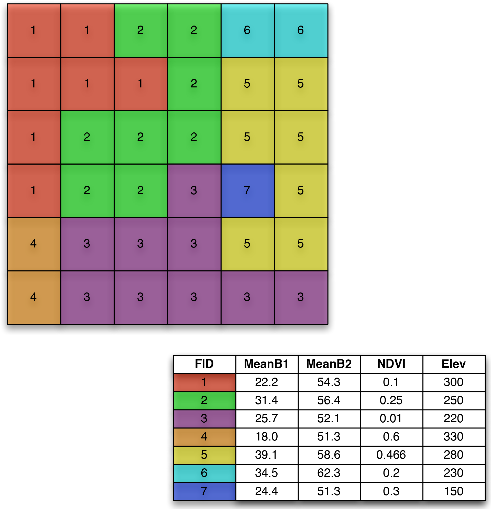
3.2. Attribute Table Creation

Once a segmentation has been created, each object is attributed with pixel values from an image (e.g., mean reflectance or backscatter) in addition to shape (e.g., length/width ratio) and contextual information (e.g., distance to neighbours), with Python functions available in RSGISLib to perform these tasks. A complete list of attributes currently available is provided in

Table 1. Available attributes for each object within the Remote Sensing and GIS Library (RSGISLib) (Version 2.1).

Image Statistics	Shape	Position	Categorical
Minimum	Area	Spatial Location	Proportion
Maximum	Length	Border	Majority (string)
Sum	Width	Distance to Feature
Mean		Distance to Neighbours
Standard Deviation
Median
Count

. The attributes are stored within the image file as an attribute table. Through GDAL, three data types are supported for storing in the RAT: integer, double and string.

3.3. Rule-Based Classification

The RIOS library is used for reading and writing the RAT in Python. Columns are read as NumPy arrays, a standard Python structure for storing multi-dimensional arrays. Through NumPy, a number of functions are available for manipulating columns (selection, slicing) and calculating statistics (min, max, mean, etc.). Mathematical operations are also supported, allowing additional attributes to be derived for each object (e.g., vegetation indices).

To perform a rule-based classification on the attribute table, the NumPy “where” statement is used for if-else statements. To develop rules, the “Select using Expression” tool within TuiView can be used, as shown in Figure 3. The NumPy syntax is used within TuiView, allowing rules to be developed using a GUI interface and then copied to a script for application. This method allows the visual assessment and adaption of complex rules with multiple combined variables, which is an advantages over other similar systems (e.g., eCognition), where variables are assessed independently.

3.4. Supervised Classification

In addition to rule-based classification, there are a number of libraries in Python to apply supervised and unsupervised classification algorithms. The Scikit-learn Python library [28], which requires data to be presented as NumPy arrays, contains a number of machine learning algorithms, including random forests, which has demonstrated good performance when applied to remote sensing data (e.g., [29]). The Scikit-learn implementation of random forests, as with many of the algorithms available, is able to utilize multiple cores for improved performance. As when applying a rule-based classification, RIOS is used to read columns from the RAT and write out the resulting classification.

4. Comparison with Other Packages

4.1. Features Overview

The system proposed was compared to existing packages providing GEOBIA functionality: OTB, InterIMAGE and eCognition. A comparison of some of the features available in each of the packages are outlined in

Table 2. A comparison of features for different Geographic Object-Based Image Analysis (GEOBIA) packages. OTB, Orfeo Toolbox.

Feature	RSGISLib	OTB + Spatial Database	InterIMAGE	eCognition
Interface	Python	Command Line Interface (CLI) / Python / Graphical User Interface (GUI)	GUI	GUI
Installation	Source (windows binaries for TuiView only).	Windows, Linux and OS X binaries, source	Windows binaries and source	Windows binaries
License	General Public License / GPL-compatible	CEA CNRS INRIA Logiciel Libre (CeCILL; Similar to GPL)	GPL	Commercial
Rule-based classification	Yes	Yes	Yes	Yes
Machine-learning classification	Through external libraries	Through external libraries	Yes	Yes
Fuzzy Classification	Not currently	Not currently	Yes	Yes
Method for storing object attributes	RAT	Spatiallite	Internal	Internal
Batch processing	Python	Python/Bash, etc.	Command line	Engine (Add on)

. Like RSGISLib, OTB does not provide all of the features required for a GEOBIA system, so it must be combined with another package. Combining the segmentation in OTB with a spatial database (e.g., PostGIS, spatiallite) to store the attributes of each object is one way of creating a complete GEOBIA system, in particular as the large-scale segmentation in OTB produces a vector output. Similarly, a spatial database could be used with RSGISLib instead of a RAT. One of the main advantage of a RAT over storing vectors in spatial database is that pixel-in-polygon operations can be performed very quickly, making operations, such as attributing objects with statistics from an image, very fast.

All systems offer the ability to perform rule-based classification. However, only eCognition and InterIMAGE are able to use membership functions to define rules; currently, this feature is not available in RSGISLib or OTB, although the implementation would be possible. A key different between packages is the interface: both InterIMAGE and eCognition are designed to be operated from a GUI and use the concept of “projects”. Although many of the functions in OTB are available through the Montverdi GUI or in QGIS through Sextante, using a GUI is not required, and the features can be accessed through a command line interface or Python bindings. In the system proposed, all of the functionality required for analysis is accessed through Python with only the GUI element (TuiView) used for data visualization and rule development, rather than analysis. Although different users may find that a GUI and “projects”-based workflow fits there specific requirements better, there are a number of advantages to a workflow based on Python scripts. Python scripts can be easily shared between users and can be used with standard version control tools (e.g., git, mercurial) to track changes made by multiple users. Applying the same processing chain to multiple images is possible with Python, as image names can be passed in as variables, making applying the same process to all images within, for example, the same directory possible using a similar script as that used to process a single image. When performing GEOBIA on an HPC, Python scripts are easy to run through job scheduling tools.

Both InterIMAGE and eCognition were designed from the ground up to be complete systems for GEOBIA. In contrast, the system proposed comprises a number of libraries, which are combined using Python, to produce a GEOBIA system. Although there are advantages to a complete system (e.g., a consistent interface, only a single program to install), the flexibility to pick and chose the best features from different packages, not limited to the ones described here, is seen as a key benefit of the system proposed and allows new algorithms to be built on top of the existing framework. Combining a number of programs, each performing a specific task, is similar to the UNIX philosophy of writing programs, which do one thing well and work with other programs.

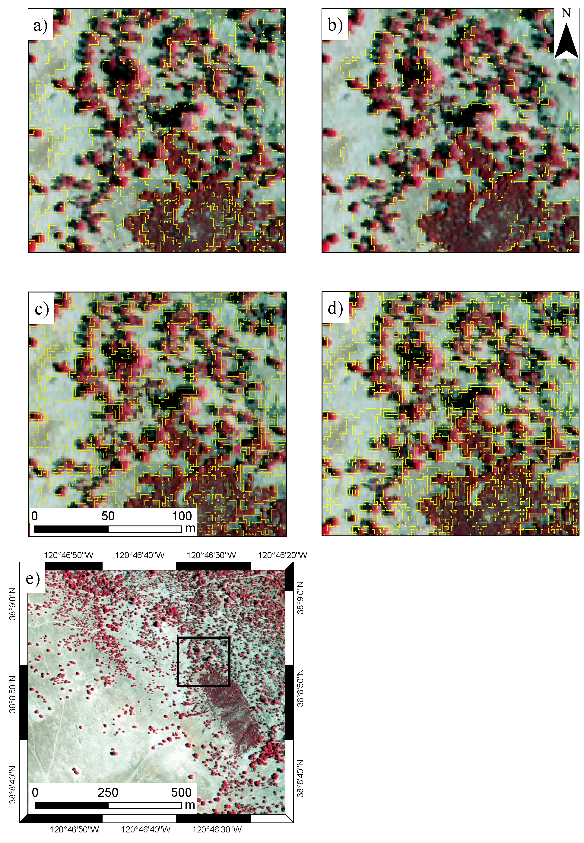
4.2. Segmentation Comparison

Segmentation is a key component in the GEOBIA processing chain. To evaluate the segmentation performance of the algorithm of Shepherd et al. [24], available in RSGISLib in relation to other packages, two test datasets were used: a 1000 × 1000 pixel, four-band, eight-bit near-infrared aerial photograph covering savanna woodland in California and a mosaic of two Landsat 8 scenes comprising seven bands with 8700 × 13,000 pixels (16-bit) covering a larger area in California and designed to test the segmentation performance over a larger dataset. The images were converted to GeoTIFF format, and overviews were generated to speed up the display. For each package, the segmentation was timed and the number of segments reported.

To compare the performance of the segmentation implementation, as RSGISLib is supported on UNIX-like platforms, eCognition is only available for Windows, and the latest binaries for InterIMAGE are only available for Windows, tests were performed using virtual machines set up with different operating systems, but the same system parameters: Quad-code 3.1 GHz i5 processor with 3 GB of RAM allocated. The amount of RAM was deliberately kept low to determine how the systems coped with images larger than the amount of available RAM, a key consideration when dealing with very large datasets. For Windows tests, Windows XP (InterIMAGE) and Windows 7 (64 bit; eCognition) were installed; for Linux tests, Ubuntu 12.04 was installed. InterIMAGE version 1.41 was used, and Windows binaries were downloaded from Laboratório de Visão Computacional (LVC). Version 9.0 of eCognition was used. The latest stable build of OTB (Version 3.2.0) was installed from the “ubuntugis” repository, as described on the OTB website. The latest version of RSGISLib (2.1.773), RIOS (1.3.0), KEA (1.4.1) and TuiView (1.1.0 beta) were installed under Linux from the source. Due to the differences in operating systems, linked libraries, compilation options, etc., the timings for each test should be seen as an indication of the “real-world” performance of each package, rather than a rigorous comparison of algorithm performance.

For OTB, the default “meanshift” algorithm was used, with all of the parameters left at the default. The large segmentation option, which produces a vector output, was used. For eCognition, the multi-resolution segmentation algorithm was used with the default scale factor of 10. For InterIMAGE, the “Baatz Segmenter” was used, with the scale parameter set to 20, as recommended in the InterIMAGE documentation. For RSGISLib, the default parameters of 60 clusters with a minimum object size of 100 pixels were used.

The segmentation time and number of segments generated by each algorithm are provided in

Table 3. A comparison of segmentation performance for four different GEOBIA packages using a small section of NIR aerial photography and a large mosaic of two Landsat 8 scenes.

Package	Small Scene		Large Scene
	Time (s)	Segments	Time (m)	Segments
RSGISLib (Linux)	11	6395	140	422,745
OTB (Linux)	24	2172	50	313,551
InterIMAGE (Windows)	50 1	16,416	-	-
eCognition (Windows)	5 1	22,400	-	1,960,447 2

¹Excludes opening image and exporting segments;

²did not complete on the test machine, and the results were generated using a different machine.

. The fastest segmentation for the aerial photograph was eCognition. However, for both eCognition and InterIMAGE, the segmentation time did not include the time to set up a project, import the data and export the segmentation. For RSGISLib, the time also includes normalizing the data, which is considered part of the segmentation algorithm. InterIMAGE was not able to segment the mosaic of two Landsat images, which exceeded the maximum supported image size. Segmenting the Landsat mosaic was not possible using eCognition on the test machine, as the algorithm relies on having sufficient RAM to process in memory. To evaluate the number of segments, a different machine was used, with a much larger amount of RAM (16 GB); the segmentation ran through successfully on this machine. As part of the segmentation in OTB, the image was split into tiles; each tile was processed on a separate thread, then the tiles were merged. For the small scene, the increased overhead meant that OTB was slower than eCognition and RSGISLib. However, for processing the large Landsat mosaic, OTB was the fastest package, as it was able to use all four cores of the test machine. Both RSGISLib and eCognition are able to utilize multiple cores by processing using tiles, but this is not considered part of the core segmentation algorithm.

The segmentation results for a subset of the aerial photography are shown in Figure 4. The results for InterIMAGE and eCognition were similar, with eCognition producing more segments. This similarity was expected, as both packages use the Baatz and Schäpe [25] segmentation algorithm, with a smaller scale parameter used in eCognition. The results for OTB and RSGISLib were similar, although more segments were produced in RSGISLib for both scenes.

The Landsat mosaic included regions without data (set to zero) outside the image footprints, both RSGISLib and OTB ignored these areas in the segmentation, while eCognition attempted to segment them. As with the aerial photography, both RSGISLib and OTB produced similar results, with RSGISLib again producing more segments. Compared to eCognition, there was more variation in object size in the segmentations produced from OTB and RSGISLib. The variation in object size was particularly evident in the Landsat mosaic, which comprised a number of large water bodies, for which both OTB and RSGISLib produced a single object, whereas eCognition split them into a number of smaller objects

It should be noted that in these tests, only the default/recommended parameters were used. In Shepherd et al. [24], it was shown that by optimizing the parameters of both RSGISLib and eCognition to maximize the segmentation quality metric of Johnson and Xie [26], similar results were obtained from both algorithms. Therefore, it is important that the parameters of any segmentation algorithm are chosen to give the best results based on the available imagery and application.

5. Examples of Use

To illustrate the application of the system described to real data, three examples, of on-going research, are presented.

5.1. Change in Mangroves Extent

The Kyoto and Carbon (K&C) initiative, Global Mangrove Watch, is aiming to map mangroves and monitor changes in mangrove extent using L-band Synthetic Aperture Radar (SAR) data from two sensors: the Japanese Earth Resources Satellite (JERS-1) and the Advanced Land Orbiting Satellite (ALOS) Phased-Array L-band SAR (PALSAR). As part of this initiative, the use of the GEOBIA system described is being investigated. To demonstrate the potential of this system and, specifically, the change detection module, a single 1° × 1° tile from the coast of French Guiana, South America, of JERS-1 data from 1996 and PALSAR data from 2007 and 2010 were used to develop an initial process for classifying mangrove change and extent. Only HH-polarization PALSAR data were used, to provide consistency with the JERS-1 SAR data. The classification and change detection was separated into three stages:

(1)

Segmentation, using data from all three years.

(2)

Rule-based classification of the 1996 data

(3)

Identification of change in the 2007 and 2010 data, relative to the 1996 baseline.

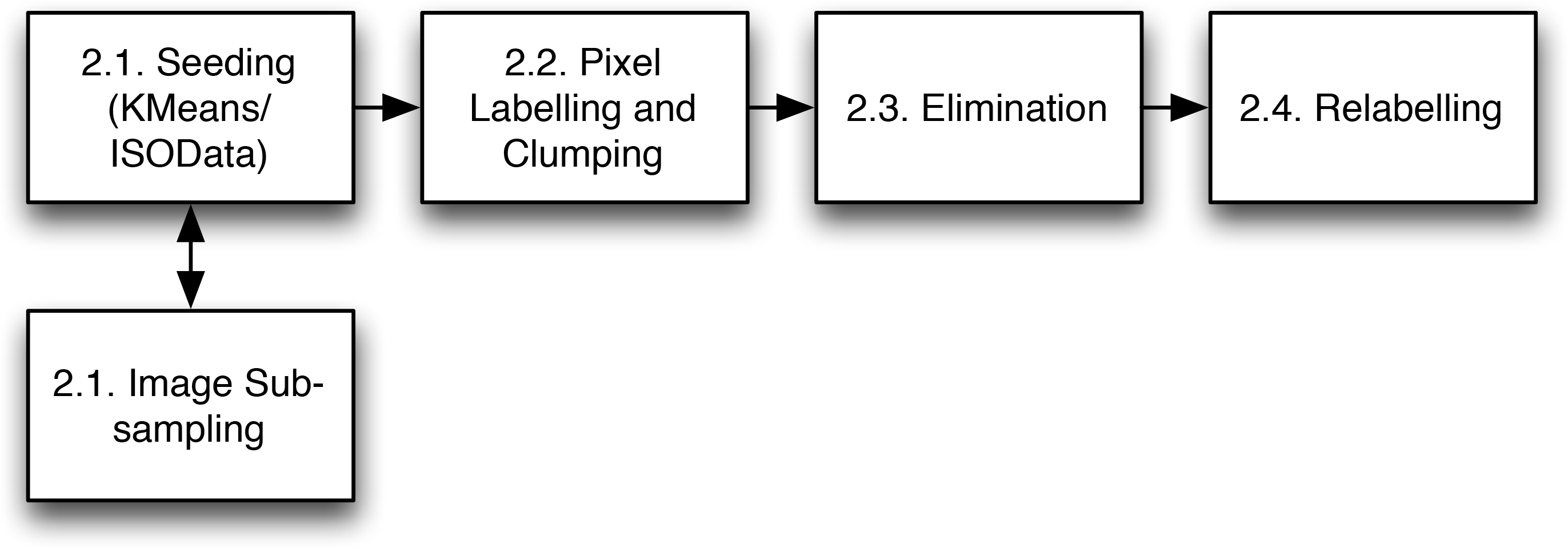
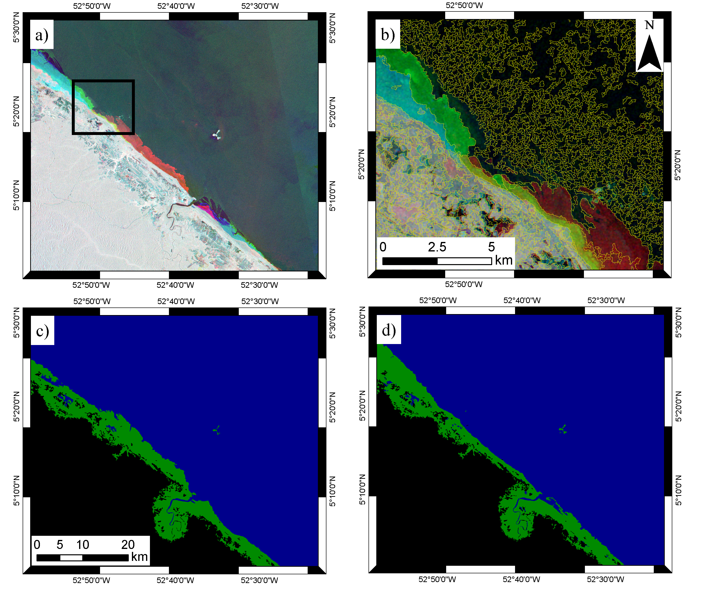
5.1.1. Segmentation

The purpose of segmentation was to define a single set of segments to be used for classification, which represented the land cover in all scenes and provided a common set of boundaries for detecting change. As input to the segmentation algorithm, a stacked HH composite (1996, 2007, 2010), that had been Lee-filtered and calibrated to dB, was used (Figure 5a). The parameters chosen for the segmentation were experimentally derived (using the V and MI metrics [24,26]); K-means was seeded with 50 cluster centres, and the elimination was run until all objects were at least 50 pixels in size. A subset of the segmentation if shown in Figure 5b.

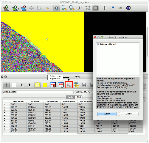
5.1.2. Rule-Based Classification

Following segmentation, a rule-based classification, where rules where experimentally derived through a visual interpretation of the imagery, was applied to produce a baseline map of mangroves from 1996. The process involved multiple steps:

(1)

Populate objects with SAR pixel statistics; where backscatter was expressed as power (linear).

(2)

Convert mean SAR backscatter to dB; for each object.

(3)

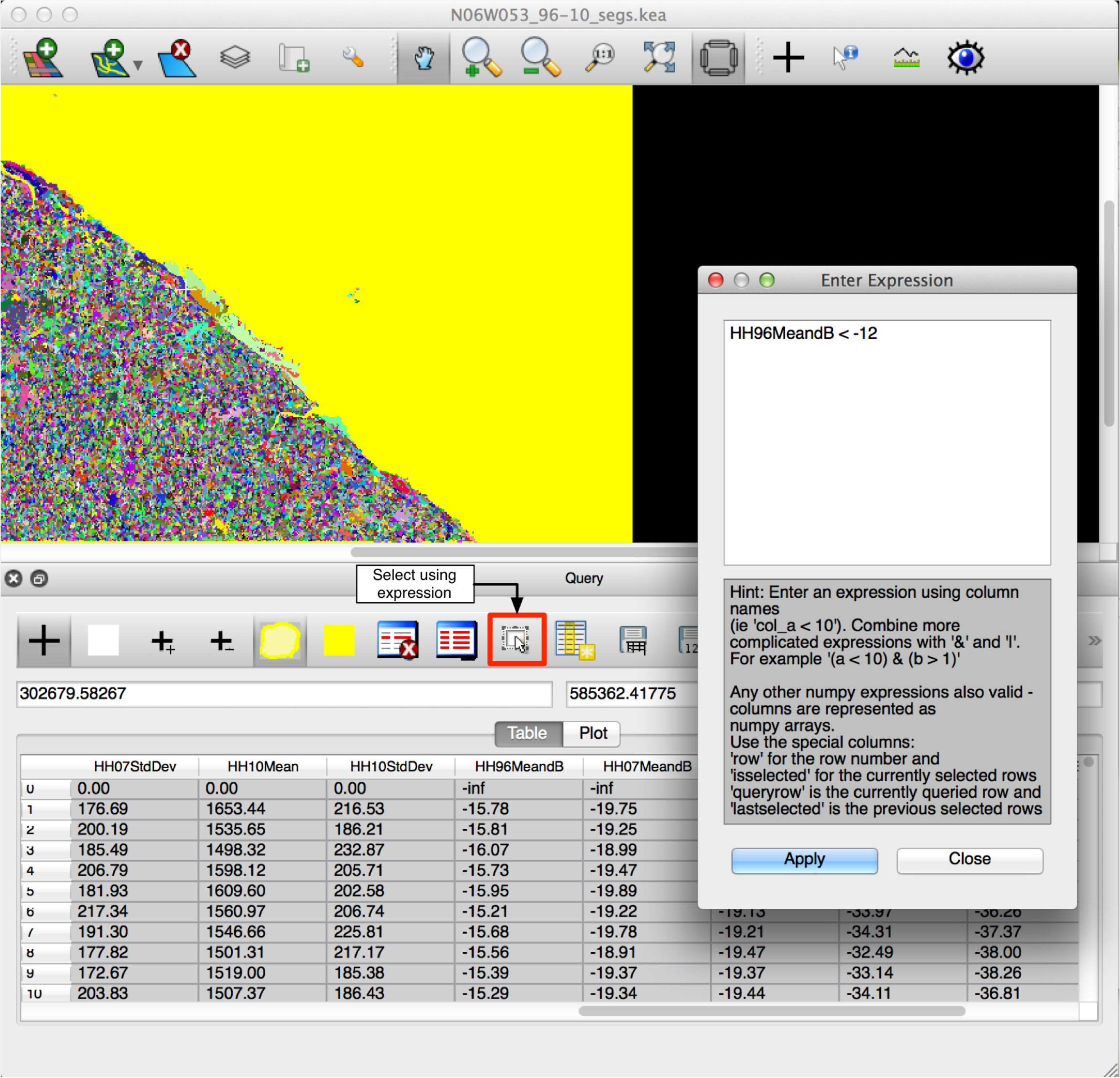
Classify water; using a threshold of < −12 dB to provide an initial mask.

(4)

Calculate the proximity to regions classified as water; to provide context for the coastal region.

(5)

Classify the scene into broad categories:

• Water (ocean); defined by selecting the largest connected water region.
• Coastal strip; defined to be within 3 km of the coast.
• Other; remaining objects not within the water of coastal strip classes.

(6)

Classify within the “coastal strip” class to identify mangroves; using a backscatter threshold.

The attribute table was populated with backscatter data for all three years, 1996, 2007 and 2010. Although a speckle-filter was applied on the data used as input for the segmentation, at the object level, an average was taken over a number of pixels, which provides a more effective way of reducing SAR speckle. Therefore, unfiltered data were used as input for the classification.

To produce an initial classification of water, a threshold of < −12 dB was applied to the HH backscatter, which was determined experimentally through an examination of object values using TuiView. In addition to the ocean, a number of other smaller clumps were classified as water. There, regions were removed using a size threshold, calculated following merging of water objects and identifying them as continuous regions.

A key criteria for identifying mangroves is the proximity to salt water. Following classification of water, objects with a proximity of less than 3 km to water were classified as coast. This created three, broad classes, water (ocean), coastal strip and the remaining objects (labeled other). Within the coastal strip class, mangroves were classified by applying different thresholds to HH-backscatter depending on the proximity to water. Closer to the coast, a lower threshold was used (> −10 dB) compared to further away from the coast (> −8 dB). A further refinement of the water classification was undertaken for segments very close (with 100 m) to the sea. The final classification is shown in Figure 5c.

5.1.3. Change Detection

Within RSGISLib, there is a change detection algorithm, which operates on objects and aims to identify segments within an existing classification that are inconsistent with the rest of the class. These segments are highlighted as either an error (in the previous classification) or true change. Segments were identified if they were a given number of standard deviations (chosen as three) from the class mean of HH-backscatter. Once possible change features were identified, they were classified, but giving consideration to classes, they were likely to change to (e.g., mangroves to water and water to mangroves). As with the original classification, the change classification rules used thresholds applied to the mean object backscatter. The process was applied to a classification from the 1996 JERS-1 data and 2007 PALSAR data, to produce a classification for 2007, which was used as a baseline to classify the 2010 PALSAR data. The classification for 2010, produced using the change detection method, is shown in Figure 5d.

The approach provided a map of mangroves and mangrove change, which compared well to manual interpretation of the SAR data and high resolution optical data available through Google Earth. However, there were some urban areas on the coast erroneously classified as mangroves. The process described illustrates how the software can be used to perform a hierarchical rule-based classification, incorporating contextual information, functions typically utilized in GEOBIA. The method for change detection is promising at the object level, and future work will look at various statistical comparisons (e.g., t-test).

To scale the approach up to map mangroves globally, different regions will be processed on separate nodes. One of the key advantages of using open source software is that it will allow the distribution of the classification process to all parties involved in the Global Mangrove Watch. In this way, refinements to the process can be made to increase the accuracy of the mapping based on local knowledge and sources of additional data.

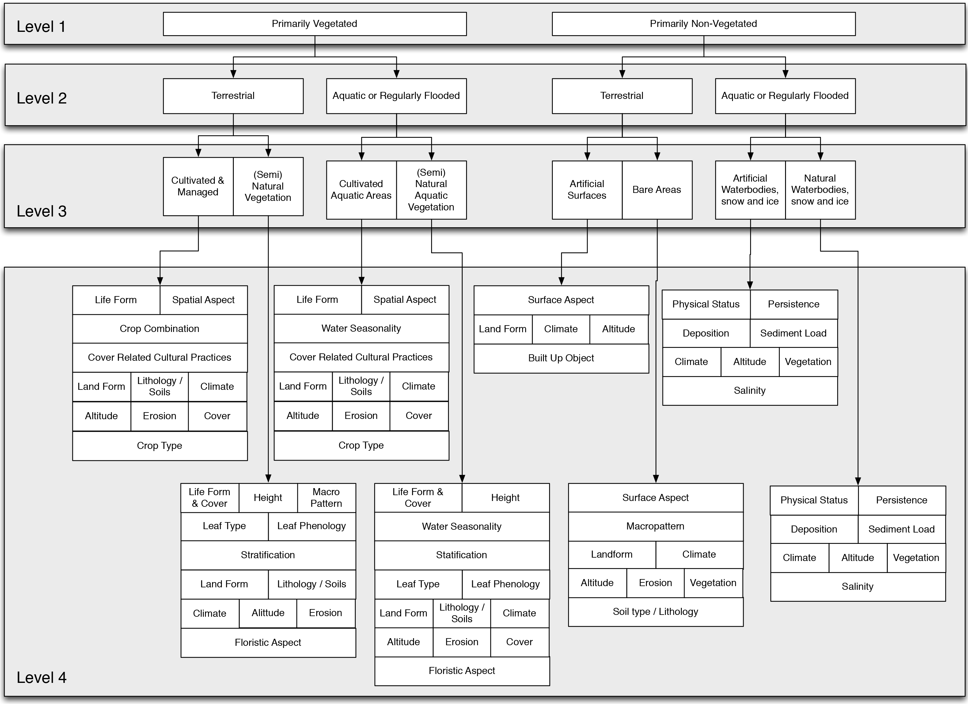
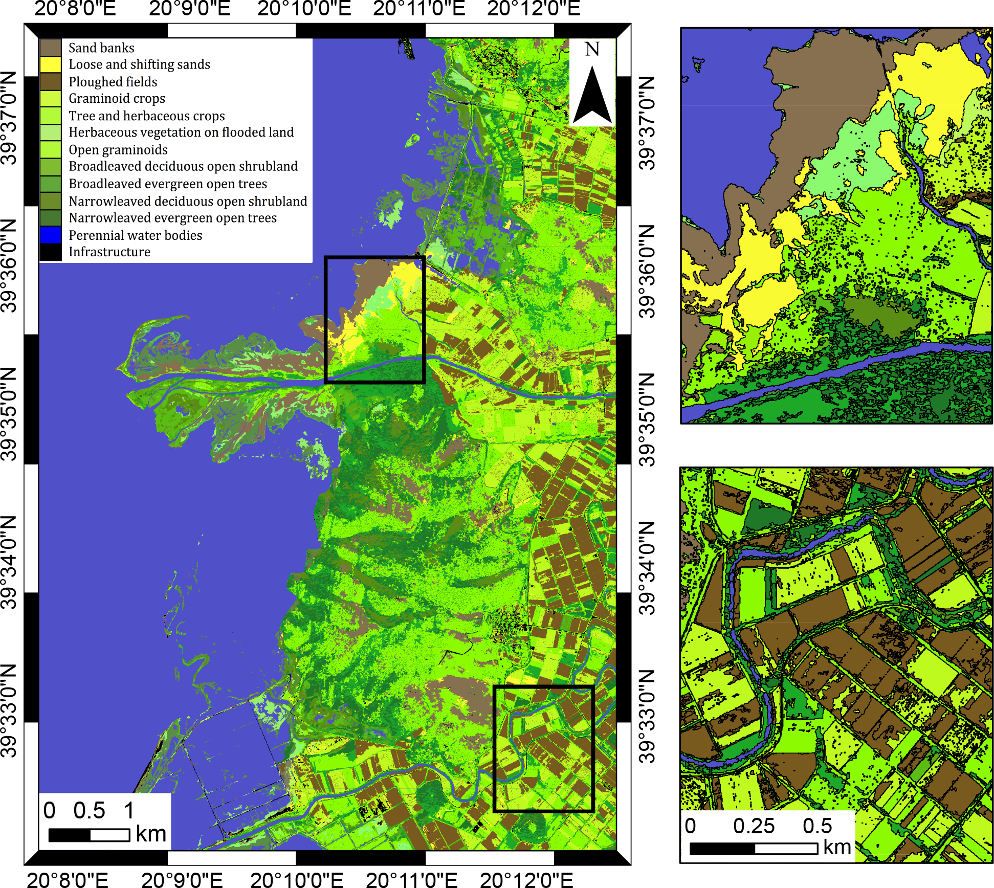
5.2. Land Cover and Habitat Classification

The EU FP7-funded BIOdiversity Mutli-SOource Monitoring System From Space to Species (BIO_SOS; http://www.biosos.eu/) project sought to develop the Earth Observation Dynamic Habitat Mapping (EODHaM) system for mapping the extent of habitats in and around protected sites (primarily Natura 2000) and highlighting changes, whether due to natural or anthropogenic causes. The taxonomy used for land cover classification was the Food and Agricultural Organization (FAOs) Land Cover Classification Scheme (LCCS; [30]) with land cover classes translated subsequently to General Habitat Classes (GHCs). A particular benefit of the classification was that it could be implemented using airborne or satellite sensor data acquired at any scale and that the classes generated were consistent and relevant globally.

The EODHaM system was developed using seasonal imagery, ideally spring (before vegetation flush) and summer (during the vegetation flush). The system is particularly suited to very high resolution multispectral imagery (e.g., Worldview-2), but lower resolution data, such as Landsat, can also be used, but with fewer classes derived. The system utilized GEOBIA throughout and is described fully in Lucas et al. [31]. To define the segments used for classification, a number of steps were undertaken:

• Feature extraction; identification and segmentation of buildings and trees using [32].
• Segmentation; application of the Shepherd et al. [24] algorithm to the scene.
• Segmentation Fusion; extracted feature boundaries, segmentation and thematic layers (e.g., roads) are fused to provide the segments to be used for the classification steps.

The segments provided a summarized representation of the environment, with the number of segments typically about 0.5 % of the number of image pixels. This significantly reduced the computational cost of the classification step(s) and allowed further features and measures of information to be used within the classification, specifically spectral variance (i.e., texture), shape and context (e.g., distance from water and slope). Individual objects were then populated with reflectance data and derived indices (e.g., the Normalized Difference Vegetation Index (NDVI), Plant Senescence Reflectance Index (PSRI) and the Water Band Index (WBI)). Where available, objects were also attributed with vegetation height and terrain slope from airborne LiDAR data to obtain information on the ground surface topography and the canopy height and structure.

The EODHaM system was then implemented as a hierarchical rule-based classification comprised of four stages (levels; Figure 6), where classification rules were defined in Python using RIOS to access the RAT for each level. TuiView was used to visually train the classification and to develop the rule base.

• Level 1 : assignment of objects to vegetated or not-vegetated classes.
• Level 2 : assignment of objects to terrestrial or aquatic classes.
• Level 3 : definition of objects to cultivated, managed or artificial or natural or semi-natural classes.
• Level 4 : description of position (e.g., soils) and type (e.g., woody).

Following the classification of each Level (1–3), the classifications were combined, giving two classes at Level 1, four at Level 2 and eight at Level 3; Figure 6. Classification beyond Level 3 was then achieved by generating approximately 30 columns within the RAT (varied depending on environment) with each representing a hierarchical component of the LCCS system. For example, different columns were established to describe vegetation on the basis of their type (woody (trees or shrubs), herbaceous (forbs or grasses) or mosses/lichens), percentage of cover, height, leaf type, phenology and stratification. An alpha-numeric code [30] was generated from each of these columns, and the final LCCS class was generated by combining these codes in a final column, with each string of codes then automatically associated with a class description.

An example classification for the Kalimas Delta, Greece, is shown in Figure 7. Through a series of logical rules, each LCCS class was translated to a General Habitat Class (GHC) [33].

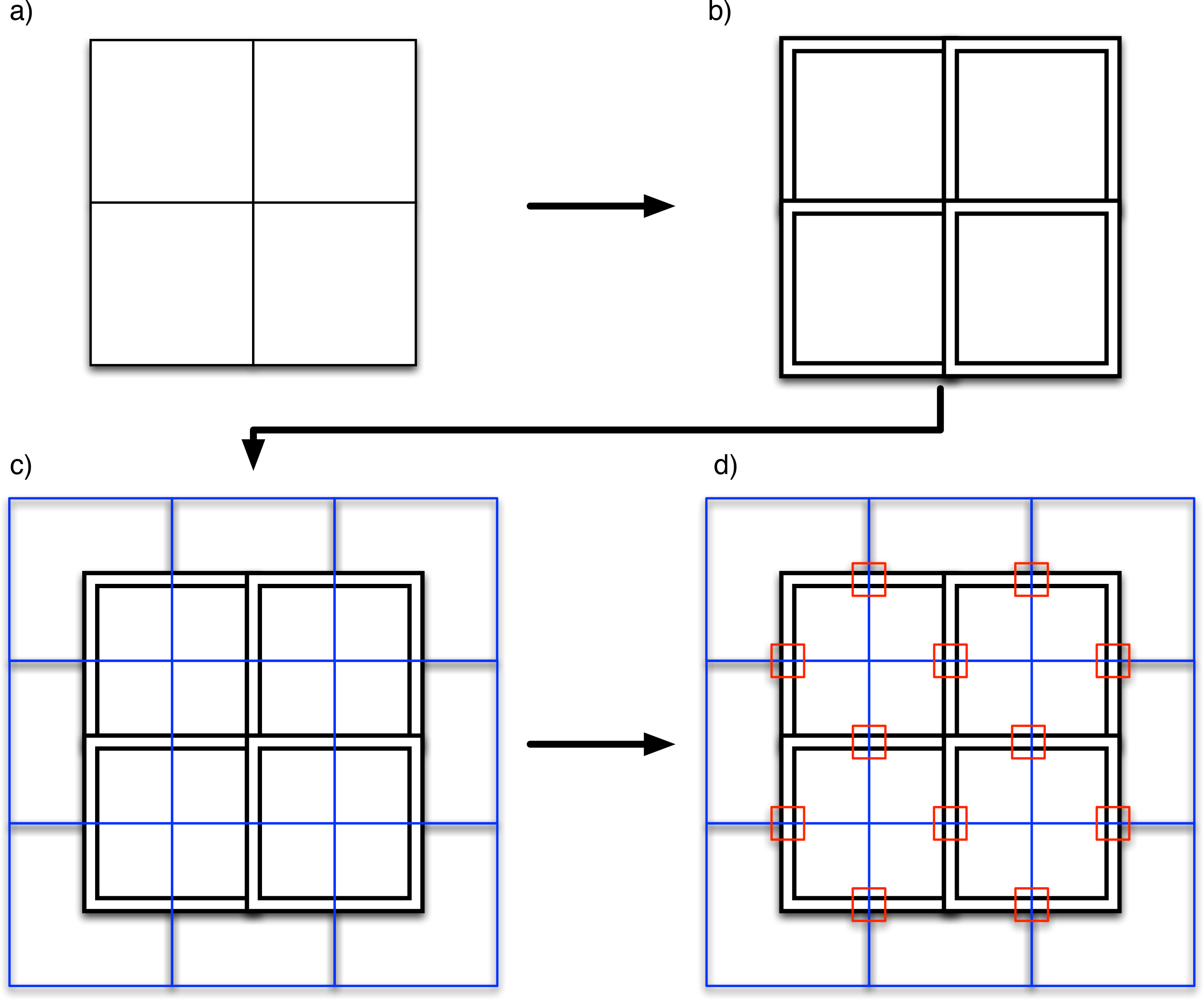
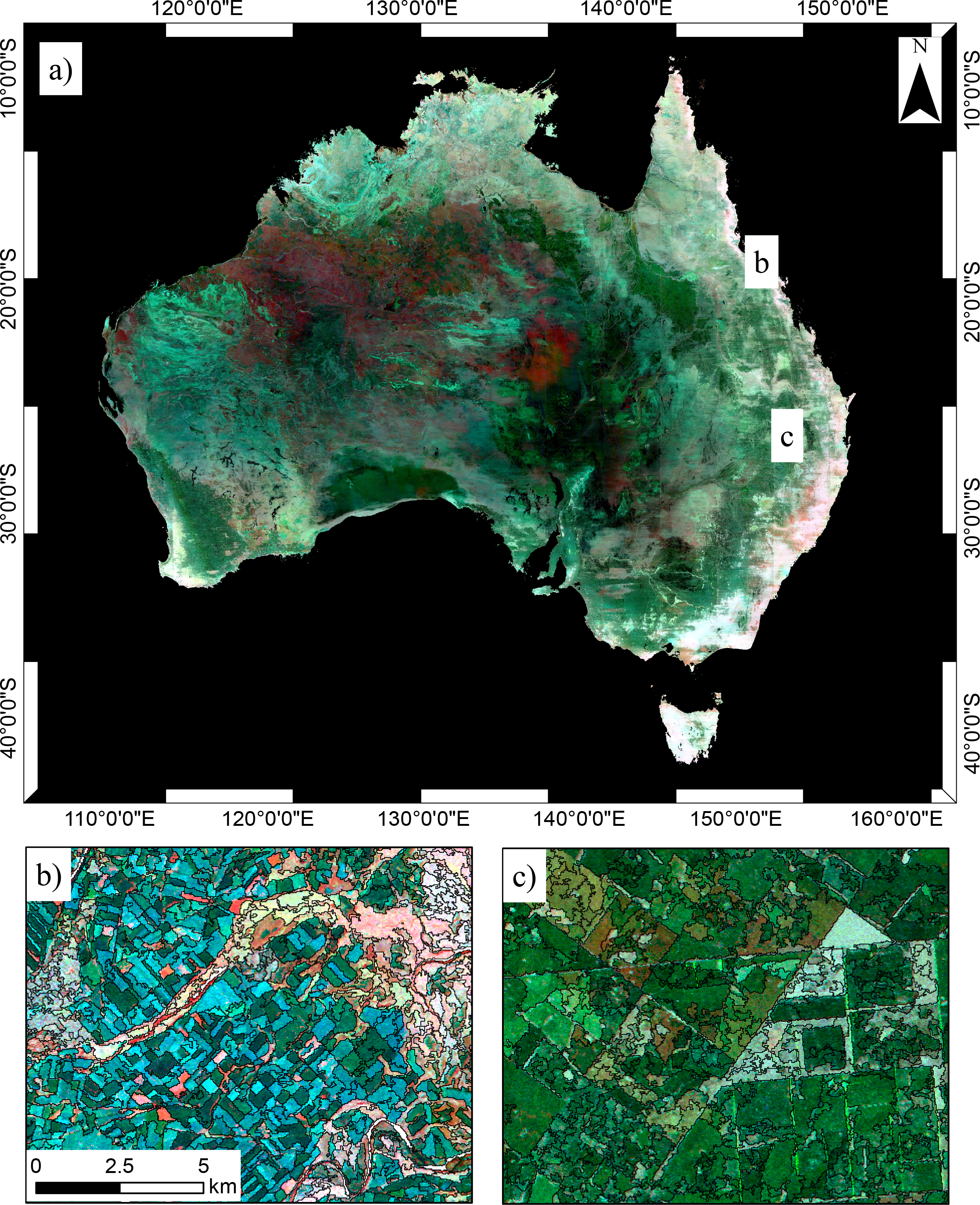
5.3. Scalable Image Segmentation

Within the field of remote sensing, the size and availability of data is becoming ever larger; in the coming years, with the recent launch of Landsat 8, and the upcoming launches of the ESA Sentinel satellites and ALOS PALSAR-2, this is going to continue to increase. To apply GEOBIA techniques to these data over large spatial areas will require software and algorithms specifically written for these applications. Within RSGISLib, the segmentation algorithm of Shepherd et al. [24] has been extended to support image tiling and the mosaicking of the segmented tiles removing the tile boundaries. Splitting the image into tiles presents problems for GEOBIA and can result in processing artefacts, such as straight lines, at tile boundaries. However, to make use of modern high performance computing (HPC) systems with a large number of processing cores, tiling in some form is a very useful function, as each tile can be independently processed on separate processing cores before being mosaicked to create the final product.

To illustrate this method, a mosaic of Landsat-derived persistent green vegetation fraction product [34,35] and PALSAR HH and HV data at 30-m resolution (141,482 × 130,103 pixels) was generated for Australia. These data were segmented in RSGISLib using the following steps (Figure 8):

• Split the data into tiles with an overlap between the tiles; tiles of 10,000 × 10,000 pixels were used, including a 500 pixel overlap.
• Segment each tile independently; utilizing multiple cores on an HPC.
• Merge the tiles, removing any segments next to the tile boundaries: the segments in contact with the tile boundary have artefacts due to the tiling.
• Split the merged segmentation into tiles, but with half a tile offset relative to the original tiles; a half tile offset is used so that the intersection of four tiles from the original segmentation will now be in the center of the new tiles.
• Segment regions on tile boundaries using the same parameters as the first segmentation; following this step, the majority of the scene will be correctly segmented with no boundary artifacts, and this relies on the segmentation always producing the same results, given the same parameters.
• Merge the segments generated at the tile boundaries into the original segmentation; during the merging process, a segment ID offset is used to ensure that segments have unique IDs.
• Finally, merge the independent regions at the boundaries of the second set of tiles, re-segment and copy into the main segmentation (Figure 8d); this produces the final result and eliminates artifacts due to the tiling process.

Segmentation took around 30 min to process each tile and less than three hours to merge all of the segments. For Australia, the final segmentation produced 33.7 million segments (Figure 9), of the same quality as the single scene segmentation using Shepherd et al. [24], which have been shown to be of comparable quality to other common segmentation algorithms. Following field visits to a number of selected sites in Queensland, it was found that the segments had a good correspondence with regions of homogeneous vegetation height and cover.

Storing the segmentation as raster clumps, rather than as a vector, allows the entire segmentation to be easily visualized, following the generation of overview layers, and allows objects to be quickly attributed with statistics from an image. For example, attributing each of the objects with mean persistent green fraction, HH and HV PALSAR backscatter took around 18 minutes and used ∼2 GB of RAM on a standard desktop computer (3.1 GHz i5, 8 GB RAM, Ubuntu 12.04; RSGISLib 2.2.850). On the same machine, viewing the entire segmentation in TuiView and getting the attributes for each segment was quick, requiring ∼1 GB of RAM.

Being able to apply a segmentation to very large area datasets and produce similar results to those obtained using small subsets is a key goal in the operational use of GEOBIA. The software presented is being used to work with large datasets and provides a consistent interface and results, moving from small test sites to national-level mapping.

6. Discussion

6.1. Expansion of the System

One of the key advantages of the system proposed, in comparison to other packages, such as eCognition [5] and InterIMAGE [12], is that its modular nature allows other packages to be incorporated alongside or instead of the existing software and for researchers to build new algorithms on top of the existing framework. The system proposed provides functions to segment an image, attribute each object and access these attributes in a memory-efficient way for visualization and analysis. Two examples of a hierarchical rule-based classification have been presented to demonstrate the system and the complexity of rule bases, which can be applied. However, the system is not restricted to rule-based classification and could be used to implement existing or new algorithms, depending on the user requirements.

The Python language is particularly beneficial in allowing the system to be expended, because: (1) there are a large number of Python libraries already available, such as pandas [36] and statsmodels [37], which provide functions for statistical analysis; (2) Python provides good interoperability with other languages, such as C/C++ and Fortran (through f2py; [38]), allowing existing code to be incorporated as part of the workflow. Presenting the attributes of each object as a NumPy arrays, through RIOS, makes it easy to interface with these packages.

6.2. License

The licenses under which all of the libraries in the system presented are released allow them to be used freely, including within a commercial setting. With the exception of the KEA library, all libraries use the GNU Public License (GPL; [39]), which is a so-called “copyleft” license, meaning that any works derived from GPL-licensed software must be released under a GPL-compatible license. Therefore, the source code of any derived software must be made available, not just binaries. To retain compatibility with GDAL, the KEA library was released under a more liberal MIT-X license, which does not place such restrictions on the availability of source code, but is still compatible with the GPL. TuiView was released under the GPLv2 license, whereas RIOS and RSGISLib use the more recent GPLv3 license, which adds a number of additional clauses [40].

The Python language, which is an integral part to the system, is available under the Python Software Foundation License (PSFL), which is also GPL-compatible [41].

6.3. Future Work

The system presented is being actively used as part of research and operational mapping strategies by the authors and their collaborators. New features and improvements to existing features are regularly being made, as the system is applied to increasingly larger datasets (e.g., recent performance improvements to raster attribute table functions in RSGISLib, based on RFC40).

7. Conclusions

A new system has been presented for performing Geographic Object-Based Image Analysis (GEOBIA) based on a number of open source (GPL-compatible) software libraries developed by the authors. All of the libraries are accessed through Python, allowing processing chains to be easily build and applied to very large datasets. Through Python, a large number of third party libraries are also available, which can easily be incorporated into the GEOBIA process, due to the open and modular nature of the system. The attributes of each object are stored as a row within a raster attribute table (RAT). To facilitate the storage and processing of very large attribute tables (over 10’s of millions of rows), a new image storage format (KEA), based on HDF5 and developed by the authors, is utilized. Changes have also be made to the underlying GDAL library by the authors to allow fast and efficient processing of RATs larger than the system memory, these have been incorporated in the recently released version 1.11 of GDAL. The system was compared to three existing packages for performing GEOBIA, and a number of key features and advances were identified:

• Built entirely on software released under open source (GPL-compatible) licenses.
• Modular, allowing the system to be customized and expanded.
• All functions are accessed through Python scripts, allowing a fully automated process to be developed.
• Allows access to all the functionality of the Python language and associated libraries (e.g., SciPy, Scikit-learn).
• Scales well to complex rule sets and large datasets.

The system is being used by a growing community of international scientists and is being actively developed with the updates made available to the community on an ongoing basis.

References

1. Blaschke, T. Object based image analysis for remote sensing. ISPRS J. Photogramm. Remote Sens 2010, 65, 2–16. [Google Scholar]
2. Gibbes, C.; Adhikari, S.; Rostant, L.; Southworth, J.; Qiu, Y. Application of object based classification and high resolution satellite imagery for Savanna ecosystem analysis. Remote Sens 2010, 2, 2748–2772. [Google Scholar]
3. Lucas, R.M.; Medcalf, K.; Brown, A.; Bunting, P.J.; Breyer, J.; Clewley, D.; Keyworth, S.; Blackmore, P. Updating the Phase 1 habitat map of Wales, UK, using satellite sensor data. ISPRS J. Photogramm. Remote Sens 2011, 66, 81–102. [Google Scholar]
4. Heumann, B.W. An object-based classification of Mangroves using a hybrid decision tree—Support vector machine approach. Remote Sens 2011, 3, 2440–2460. [Google Scholar]
5. Definiens. In eCognition Version 9 Object Oriented Image Analysis User Guide; Technical report; Trimble; Munich, Germany, 2014.
6. Vu, T. Object-Based Remote Sensing Image Analysis with OSGeo Tools. Proceedings of FOSS4G Southeast Asia 2012, Johor Bahru, Malaysia, 18–19 July 2012; pp. 79–84.
7. Moreno-Sanchez, R. Free and Open Source Software for Geospatial Applications (FOSS4G): A mature alternative in the geospatial technologies arena. Trans. GIS 2012, 16, 81–88. [Google Scholar]
8. Steniger, S.; Hay, G. Free and open source geographic information tools for landscape ecology. Ecol. Inf 2009, 4, 183–195. [Google Scholar]
9. Christophe, E.; Inglada, J. Open source remote sensing: Increasing the usability of cutting-edge algorithms. IEEE Geosci. Remote Sens. Soc. Newsl 2009, 150, 9–15. [Google Scholar]
10. Inglada, J.; Christophe, E. The Orfeo Toolbox Remote Sensing Image Processing Software. Proceedings of the 2009 IEEE International Geoscience and Remote Sensing Symposium, Cape Town, South Africa, 12–17 July 2009; pp. IV-733–IV-736.
11. Huth, J.; Kuenzer, C.; Wehrmann, T.; Gebhardt, S.; Tuan, V.Q.; Dech, S. Land cover and land use classification with TWOPAC: Towards automated processing for pixel- and object-based image classification. Remote Sens 2012, 4, 2530–2553. [Google Scholar]
12. InterImage. InterImage User Manual, Version 1.41; Laboratório de Visão Computacional: Rio de Janeiro, Brazil, 2014. [Google Scholar]
13. Gillingham, S.; Bunting, P. RFC40. Available online: http://trac.osgeo.org/gdal/wiki/rfc40_enhanced_rat_support (accessed on 24 March 2014).
14. Bunting, P.; Clewley, D.; Lucas, R.M.; Gillingham, S. The Remote Sensing and GIS Software Library (RSGISLib). Comput. Geosci 2014, 62, 216–226. [Google Scholar]
15. Bunting, P. ARCSI. Available online: https://bitbucket.org/petebunting/arcsi (accessed on 25 January 2014).
16. Wilson, R.T. Py6S: A Python interface to the 6S radiative transfer model. Comput. Geosci 2013, 51, 166–171. [Google Scholar]
17. Vermote, E.; Tanre, D.; Deuze, J.; Herman, M.; Morcrette, J. Second simulation of the satellite signal in the solar spectrum, 6S: An overview. IEEE Trans. Geosci. Remote Sens 1997, 35, 675–686. [Google Scholar]
18. Gillingham, S.; Flood, N. RIOS. Available online: https://bitbucket.org/chchrsc/rios/ (accessed on 25 January 2014).
19. NumPy. Available online: http://www.numpy.org (accessed on 25 January 2014).
20. Jones, E.; Oliphant, T.; Peterson, P. SciPy: Open source scientific tools for Python. 2001. Available online: http://www.scipy.org (accessed on 25 June 2014).
21. Bunting, P.; Gillingham, S. The KEA image file format. Comput. Geosci 2013, 57, 54–58. [Google Scholar]
22. Zlib. Available online: http://www.zlib.net (accessed on 9 May 2014).
23. Baatz, M.; Hoffmann, C.; Willhauck, G. Progressing from Object-Based to Object-Oriented Image Analysis. In Object-Based Image Analysis; Blaschke, T., Lang, S., Hay, G., Eds.; Springer: Berlin/Heidelberg, Germany, 2008; pp. 29–42. [Google Scholar]
24. Shepherd, J.D.; Bunting, P.; Dymond, J.R. Operational large-scale segmentation of imagery based on iterative elimination. J. Appl. Remote Sens 2014, in press.. [Google Scholar]
25. Baatz, M.; Schäpe, A. Multiresolution segmentation: An optimization approach for high quality multi-scale image segmentation. J. Photogramm. Remote Sens 2000, 58, 12–23. [Google Scholar]
26. Johnson, B.; Xie, Z. Unsupervised image segmentation evaluation and refinement using a multi-scale approach. ISPRS J. Photogramm. Remote Sens 2011, 66, 473–483. [Google Scholar]
27. Christophe, E.; Inglada, J. Robust Road Extraction for High Resolution Satellite Images. Proceedings of the IEEE International Conference on Image Processing (ICIP 2007), San Antonio, TX, USA, 16–19 September 2007.
28. Pedregosa, F.; Varoquaux, G.; Gramfort, A.; Michel, V.; Thirion, B.; Grisel, O.; Blondel, M.; Prettenhofer, P.; Weiss, R.; Dubourg, V.; et al. Scikit-learn: Machine learning in Python. J. Mach. Learn. Res 2011, 12, 2825–2830. [Google Scholar]
29. Gislason, P.O.; Benediktsson, J.A.; Sveinsson, J.R. Random forests for land cover classification. Pattern Recognit. Lett 2006, 27, 294–300. [Google Scholar]
30. Di Gregorio, A.; Jansen, L. Land Cover Classification System (LCCS): Classification Concepts and User Manual for Software, Version 2; Technical Report 8; FAO Environment and Natural Resources Service Series: Rome, Italy, 2005. [Google Scholar]
31. Lucas, R.; Bunting, P.; Jones, G.; Arias, M.; Inglada, J.; Kosmidou, V.; Petrou, Z.; Manakos, I.; Adamo, M.; Tarantino, C.; et al. The Earth Observation Data for Habitat Monitoring (EODHaM) system. JAG Int. J. Appl. Earth Obs. Geoinforma. Special Issue Earth Obs, 2014; in press. [Google Scholar]
32. Arias, M.; Inglada, J.; Lucas, R.; Blonda, P. Hedgerow Segmentation on VHR Optical Satellite Images for Habitat Monitoring. Proceedings of the 2013 IEEE International Geoscience and Remote Sensing Symposium (IGARSS), Melbourne, Australia, 21–26 July 2013; pp. 3301–3304.
33. Kosmidou, V.; Petrou, Z.; Bunce, R.G.; Mücher, C.A.; Jongman, R.H.; Bogers, M.M.; Lucas, R.M.; Tomaselli, V.; Blonda, P.; Padoa-Schioppa, E.; et al. Harmonization of the Land Cover Classification System (LCCS) with the General Habitat Categories (GHC) classification system. Ecol. Indic 2014, 36, 290–300. [Google Scholar]
34. Gill, T.; Johansen, K.; Scarth, P.; Armston, J.; Trevithick, R.; Flood, N. AusCover Good Practice Guidelines: A Technical Handbook Supporting Calibration and Validation Activities of Remotely Sensed Data Products. Available online: http://data.auscover.org.au/xwiki/bin/view/Good+Practice+Handbook/PersistentGreenVegetation (accessed on 25 June 2014).
35. Scarth, P. Persistent Green-Vegetation Fraction and Wooded Mask—Landsat, Australia Coverage. Available online: http://www.auscover.org.au/xwiki/bin/view/Product+pages/Persistent+Green-Vegetation+Fraction (accessed on 15 February 2013).
36. McKinney, W. Data Structures for Statistical Computing in Python. Proceedings of the 9th Python in Science Conference, Austin, TX, USA, 28 June–3 July 2010; pp. 51–56.
37. Seabold, J.; Perktold, J. Statsmodels: Econometric and Statistical Modeling with Python. Proceedings of the 9th Python in Science Conference, Austin,TX, USA, 28 June–3 July 2010.
38. Peterson, P. F2PY: A tool for connecting Fortran and Python programs. Int. J. Comput. Sci. Eng 2009, 4, 296–305. [Google Scholar]
39. 2007. GNU. GNU General Public License (GPL) Version 3. Available online: http://www.gnu.org/copyleft/gpl.html (accessed on 10 April 2014).
40. Institute for Legal Questions on Free and Open Source Software. Available online: http://www.ifross.org/en/what-difference-between-gplv2-and-gplv3 (accessed on 10 April 2014).
41. Free Software Foundation. Available online: http://www.gnu.org/licenses/license-list.html (accessed on 26 January 2014).
Figure 1. Example of raster clumps, used to store a represented object, and the corresponding attribute table. Each clump is linked to a row in the attribute table by the pixel values, which correspond to the clump feature ID (FID).
Remotesensing 06 06111f1
Figure 2. The Shepherd et al. [24] segmentation algorithm. First, K-means clustering is used to generate seeds for the segmentation, optionally sub-sampling the data. Following the assignment of the pixels to the associated cluster center, the clumps are iteratively eliminated if they are below the minimum mapping unit threshold to the neighbouring clump that is closest in “colour” (defined through Euclidean distance). Following elimination, the final clumps are relabelled to ensure that they are consecutively numbered.
Remotesensing 06 06111f2
Figure 3. A screen shot showing how TuiView is used to interrogate the raster attribute table (RAT) through the “Select using Expression” tool to interactively define thresholds for a rule-based classification.
Remotesensing 06 06111f3
Figure 4. A comparison of segmentation results (yellow outline) using different packages applied to a test dataset of near-infrared aerial photography over wooded savanna in California, U.S. Results shown for a subset segmented using (a) RSGISLib, (b) OTB, (c) InterIMAGE and (d) eCognition. The full image is shown in (e).
Remotesensing 06 06111f4
Figure 5. Classification of mangroves change using Japanese Earth Resources Satellite (JERS-1) and the Advanced Land Orbiting Satellite (ALOS) Phased-Array L-band SAR (PALSAR) data: (a) color composite of JERS-1 data from 1996 (red) and PALSAR data from 2007 (green) and 2010 (blue); (b) subset of scene showing segmentation; (c) classification of mangroves (green) using 1996 data; (d) updated classification of mangroves using 2010 data.
Remotesensing 06 06111f5
Figure 6. The hierarchical structure of Levels 1 to 4 of the Land Cover Classification Scheme (LCCS; [30]), implemented using the GEOBIA system proposed.
Remotesensing 06 06111f6
Figure 7. Classification of the Kalimas Delta, Greece, using the Earth Observation Dynamic Habitat Mapping (EODHaM) system. Subsets show the outlines of merged objects for each class.
Remotesensing 06 06111f7
Figure 8. To segment large area datasets, processing was undertaken in three steps: (a) tiling and segmentation of the tiles; (b) Identification of boundary objects in the segmented tiles; (c) generating a mask defining regions of boundary objects, retiling with half a tile offset and re-segmentation of the masked regions; (d) finally, the remaining isolated boundary regions within the red squares are identified and individually re-segmented.
Remotesensing 06 06111f8
Figure 9. A national-scale segmentation of Australia derived from a composite of persistent green fraction [34] and Advanced Land Orbiting Satellite (ALOS) PALSAR data with a spatial resolution of 30 m. (a) Overview of the entire segmentation with each object coloured using the mean persistent green fraction product (red), and ALOS PALSAR HH (green) and HV (blue) backscatter. Subsets (b,c) show the objects in detail over-persistent green fraction and PALSAR data.
Remotesensing 06 06111f9