Moving Vehicle Information Extraction from Single-Pass WorldView-2 Imagery Based on ERGAS-SNS Analysis

Abstract

Due to the fact that WorldView-2 (WV2) has a small time lag while acquiring images from panchromatic (PAN) and two multispectral (MS1 and MS2) sensors, a moving vehicle is located at different positions in three image bands. Consequently, such displacement can be utilized to identify moving vehicles, and vehicle information, such as speed and direction can be estimated. In this paper, we focus on moving vehicle detection according to the displacement information and present a novel processing chain. The vehicle locations are extracted by an improved morphological detector based on the vehicle’s shape properties. To make better use of the time lag between MS1 and MS2, a band selection process is performed by both visual inspection and quantitative analysis. Moreover, three spectral-neighbor band pairs, which have a major contribution to vehicle identification, are selected. In addition, we improve the spatial and spectral analysis method by incorporating local ERGAS index analysis (ERGAS-SNS) to identify moving vehicles. The experimental results on WV2 images showed that the correctness, completeness and quality rates of the proposed method were about 94%, 91% and 86%, respectively. Thus, the proposed method has good performance for moving vehicle detection and information extraction.

1. Introduction

Vehicle monitoring is one of the key issues for modeling and planning for traffic and transportation management for terrestrial areas [1]. Recently, the use of remote sensing data for vehicle monitoring has become an attractive field of research. Most high resolution optical observation satellites carry panchromatic (PAN) and multispectral (MS) sensors onboard. PAN and MS sensors are assembled at different positions on the focal plane unit. Due to this configuration, there is a short time lag between the acquisition of PAN and MS images. Thus, a moving vehicle is observed at different positions in a single set of satellite imagery. Most optical satellite images, such as IKONOS, QuickBird, WorldView-2 and GeoEye-1, have such properties. If we can precisely calculate the displacement of a moving vehicle during the time lag, the speed and moving directions of the vehicle can be estimated. This is the fundamental rationale of the moving vehicle detection by using a single set of satellite imagery [2].

Various methods have been developed for vehicle detection from remote sensing images, and these methods can be classified into two categories: appearance-based model and temporal change-detection-based model. Most vehicle detection methods use an appearance-based model to extract the blob-like structure of vehicles. Some methods use aerial images with a resolution in the range of 15–30 cm. Typical vehicles have a length of 15–30 pixels, and then, the detailed appearance and shape of vehicles are visible in these images. These methods often build an explicit appearance model [3–5] for vehicle extraction. However, satellite images have relatively lower resolution compared with aerial images; thus, an explicit appearance-based model [3–5] is not appropriate for satellite images. Therefore, many studies based on satellite images (QuickBird, WorldView-2, etc.) use a blob detection algorithm for vehicle detection. Leitloff et al. use adaptive boosting combined with Haar-like features to detect vehicles in urban areas [6]. Larsen et al. proposed an elliptical blob detection strategy followed by region growing and feature extraction to detect vehicles on suburban roads [7]. Eikvil et al. proposed a classification-based method to exploit the spatial and gray level features of vehicles on city roads and highways [8]. These methods have shown impressive performance. However, vehicle movement information cannot be extracted by appearance analysis.

On the other hand, some methods use a temporal change-detection-based model for vehicle extraction. The time gap between image acquisitions of sensor band groups is exploited; thus, the speed and direction of a moving vehicle can be estimated. Many methods employ QuickBird or IKONOS images to exploit the tiny time gap between PAN and MS sensors. Zhang and Xiong first proposed a moving vehicle detection method by using the time gap between multispectral and panchromatic bands of QuickBird images [2]. Easson et al. used image differencing to recognize vehicles in motion [9]. Liu et al. developed an area correlation method to estimate the speed of moving vehicles [10]. Krauß et al. proposed a method to estimate the exact time gap between the acquisitions of the different bands of RapidEye, and then, the speed of moving object could be estimated [11]. Meanwhile, with the advent of WorldView-2 (WV2), new methods have been developed to exploit the special focal plane assembly by WV2. The WV2 satellite carries a panchromatic (PAN) and two multispectral (MS1 and MS2) sensors onboard. Due to the hardware arrangement, the sequence of collected images is MS1, PAN and MS2 [1]. Hence, a moving vehicle is observed at three different positions by the satellite. Salehi et al. presented a method by using the standard principal component analysis (PCA) to detect the moving vehicles’ location changes in MS1 and MS2 images [1]. Bar et al. proposed a spectral and spatial (SNS) approach to detect moving vehicles in WV2 images [12]. In both methods, all of the eight spectral bands of WV2 are used to analyze moving vehicles. However, there may be big spectral differences between some spectrally-neighboring bands, and the spectral differences may influence the detection accuracy.

Appearance-based methods can hardly extract moving vehicle information, while temporal change-detection-based methods ignore the big spectral difference between some spectrally-neighboring bands. To address the problem, we present a novel processing chain for the moving vehicle extraction of suburban roads and highways by using WV2 images. The contributions of this paper are three-fold: First, in order to capture the elliptical blob appearance of vehicles, we propose an improved morphological detector based on vehicle shape properties to extract vehicles’ candidate locations. Second, we perform a band selection process by visual inspection and quantitative analysis, and three band pairs appropriate for vehicle identification are selected. Third, we improve the SNS method by incorporating local Erreur Relative Globale Adimensionnelle de Synthese (ERGAS) analysis. Through ERGAS analysis, moving vehicles turn to bright spot pairs. The special feature reduces the exhaustive burden of SNS method, and therefore, many false alarms are eliminated. We implement the proposed method on WV2 images, and the experimental results show the good performance of the proposed method.

2. Methodology

In this paper, we are mainly focusing on two types of roads: suburban roads and highways. Suburban roads are characterized as narrow and with very low traffic density. Highways are characterized as wide and with high traffic density. Since vehicles maintain a high speed on highways, there is always an appropriate distance between two vehicles.

The proposed method consists of an automatic processing chain. The required input is WV2 images and road vector data. The flow diagram of our method is shown in Figure 1. As a first step, roads are extracted by geo-referencing image to road vector data. Vegetation and shadow regions are eliminated to reduce false-alarm hypotheses. Then, we use an improved top-hat transformation to get the vehicles’ candidate locations. The next step is to identify moving vehicles. We perform band selection by both visual inspection and quantitative analysis, and three spectral band pairs appropriate for moving vehicle identification are selected. Then, a SNS method incorporating the ERGAS analysis (ERGAS-SNS) approach is utilized to identify moving vehicles. Finally, the vehicle’s displacement between MS1 and MS2 images can be extracted by ERGAS-SNS analysis. The speed and directions of movement are then calculated using the displacement and the time lag between MS1 and MS2 images.

2.1. Road Extraction

Based on the assumption that vehicles are moving along the road, a road extraction procedure is employed as the preprocessing step. This step reduces the search area and the number of false-alarm hypotheses. The road extraction is comprised of two steps: image-to-vector geo-referencing, vegetation and shadow removal. In road extraction, the required input is PAN image, MS1 image and road vector data. To facilitate the discussion, we give a general introduction to image-to-vector geo-referencing. We follow that with an introduction on how to remove vegetation and shadows.

WV2 images have latitude and longitude information to provide true ground locations, and precise road information data can be obtained conveniently for all developed countries. Therefore, it makes sense to include such data to obtain coarse road regions. In Leitloff’s work [6], road networks from the German Authoritative Topographic Cartographic Information System (ATKIS) database have been used. Such a geographic information system (GIS) database can provide vector data information of the road mid-line accompanied with a parameter representing the width of the road. Hence, by geo-referencing the vector data and PAN image, road masks can be generated automatically. The road masks can be utilized to restrict vehicle extraction to road regions. The geo-referencing step is shown in Figure 2.

Vegetation that may block parts of the roads includes the crowns of trees by the road side and plants growing in-between different lanes. In order to remove false-alarm hypotheses generated by vegetation, a vegetation mask was generated from the multispectral bands. By using the MS1 image, the normalized difference vegetation index (NDVI) is first computed. An appropriate threshold from the application of Otsu’s algorithm [13] is selected for the resulting NDVI image, and then, the vegetation mask is produced.

In addition to vegetation mask, a shadow mask is also applied. In this paper, successive thresholding scheme (STS) [14] is applied to detect shadows. The MS1 image is first transformed into a photometric invariant color model. The ratio of the hue over the intensity for each pixel is then calculated to construct the ratio map. A global thresholding process is first performed to obtain the coarse-shadow map, which separates all of the pixels of the input image into candidate shadow pixels and non-shadow pixels. Furthermore, a local thresholding process is applied to each candidate shadow region in the coarse-shadow map iteratively to distinguish real shadow pixels. It has to be noted that some dark vehicles have similar spectral properties with shadows, and these vehicles may be incorrectly classified to shadows. Hence, regions smaller 25 pixels (about the size of a vehicle) are removed from the extracted shadow regions. In the end, the vegetation and shadow masks are combined to produce a masked image. As shown in Figure 3, in the result image, all vegetation and shadow pixels that belong to coarse road regions are set to black.

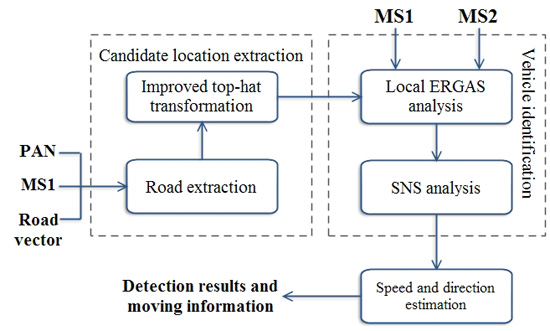
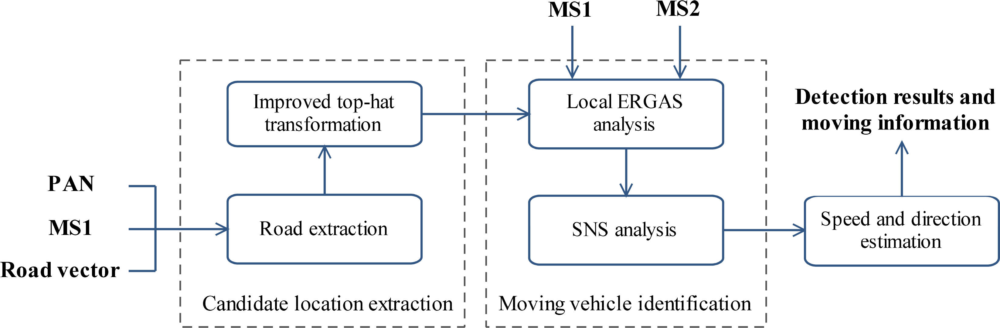
2.2. Vehicle Candidate Location Extraction

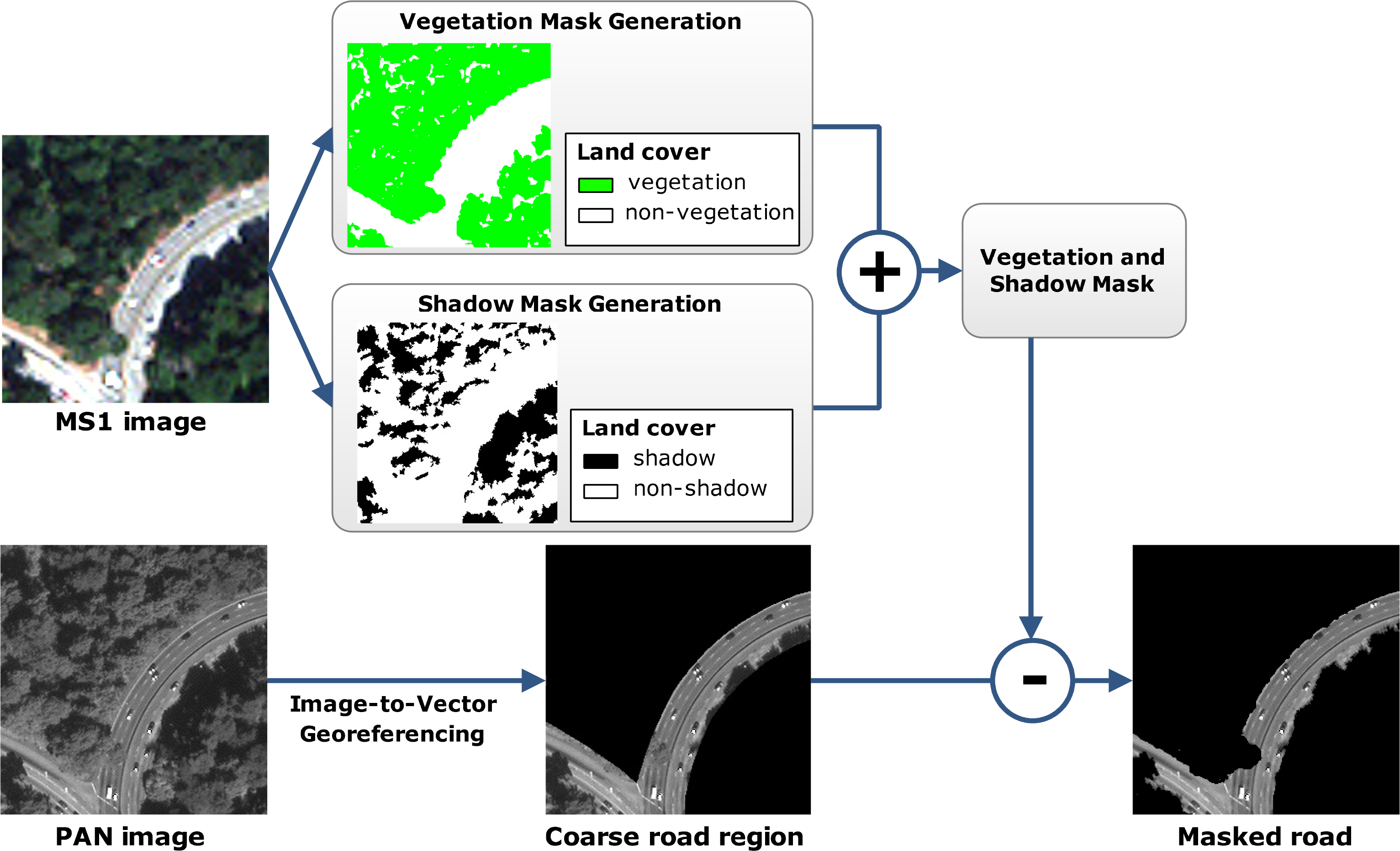
Given the road regions of the WV2 image, the first step is to locate potential vehicles. In this research, we use the PAN image to extract vehicle candidate locations. To simply and efficiently extract vehicles embedded in a cluttered background, the image is first enhanced by Perona–Malik anisotropic diffusion. This is important, because noise is reduced without the removal of significant parts of the vehicles’ information. After that, an improved top-hat transformation based on the vehicles’ appearance properties is utilized to extract moving vehicle candidate locations.

Perona and Malik diffusion is a nonlinear diffusion filtering technique. Nonlinear diffusion filtering describes the evolution of the luminance of an image through increasing scale levels as the divergence of a certain flow function that controls the diffusion process [15]. The following equation shows the classic nonlinear diffusion formulation:

$$\frac{\partial I}{\partial t}=\mathit{div}\left(c\left(x,y,t\right)\nabla I\right)$$

(1)

where div denotes the divergence operator, Δ denotes the gradient operator and c(x,y,t) is the diffusion equation. c(x,y,t) controls the rate of diffusion and is usually chosen as a function of the image gradient to preserve edges in the image. The time t is the scale parameter, and larger values lead to simpler image representations.

Perona and Malik [16] pioneered the idea of nonlinear diffusion and make c(x,y,t) dependent on the gradient magnitude to reduce the diffusion at the location of edges, encouraging smoothing within a region instead. The diffusion equation is defined as:

$$c\left(x,y,t\right)=g\left(\left|\nabla I_{\sigma }\left(x,y,t\right)\right|\right)$$

(2)

where the function ∇I_σ is the gradient of a Gaussian smoothed version of the original image I . Perona and Malik proposed two different formulations for g:

$$g_1=exp\left(-\frac{{\left|\nabla I_{\sigma }\right|}^2}{k^2}\right)$$

(3)

$$g_2=\frac{1}{1+\frac{{\left|\nabla I_{\sigma }\right|}^2}{k^2}}$$

(4)

where the parameter k controls the sensitivity to edges. The function g₁ gives privilege to wide regions over smaller ones, and the function g₂ privileges high-contrast edges over low-contrast ones.

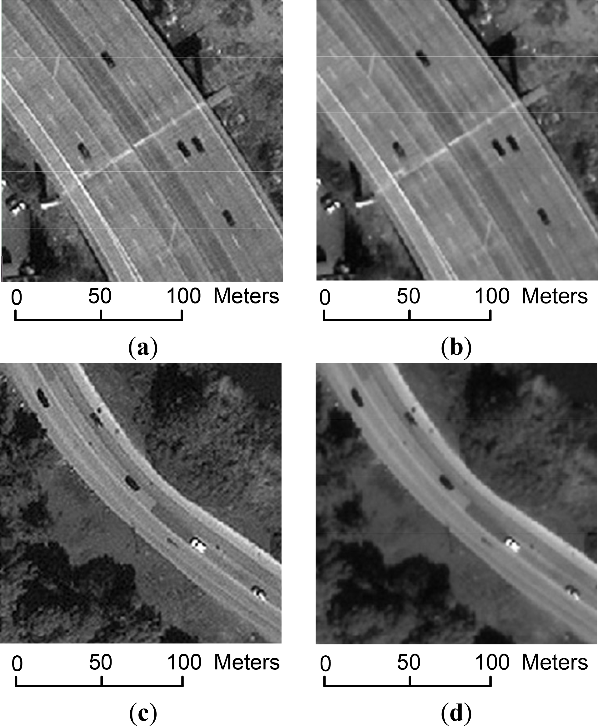
In this paper, we chose g₁ as the diffusion equation, since we want to remove undesirable noise without blurring or dislocating meaningful vehicle edges. As can be seen from Figure 4, the image is smoothed and the boundaries of vehicles are well preserved.

In the PAN image, vehicles appear to be elliptical blobs, and the idea of a blob detection algorithm for vehicle detection has been attempted [5,7]. In Zheng’s work [5], classical top-hat transformation is used to identify moving vehicles in very high resolution aerial image (0.15 m). The classical top-hat transformation is based on two morphology operations: opening and closing. The opening and closing operations are defined as:

$$f\circ b=\left(f\ominus b\right)\oplus b$$

(5)

$$f•b=\left(f\oplus b\right)\ominus b$$

(6)

where f is the original image, b is the structure element, ◦ denotes the grayscale opening transformation and • denotes the grayscale closing transformation. ⴱ and ⴲ denote the erosion operator and dilation operator, respectively. Then white top-hat transformation and black top-hat transformation, denoted by WTH and BTH, respectively, are defined as:

$$\text{WTH}:T=f-f\circ b$$

(7)

$$\text{BTH}:B=f•b-f$$

(8)

where T is the image after the WTH transformation and B is the image after BTH transformation.

WTH finds the bright regions in the image, while BTH finds dark regions. Vehicles are usually elliptical bright (dark) blobs in panchromatic images, and WTH and BTH can be directly used to find a moving vehicle. However, the classical top-hat transformation cannot differentiate the heavy clutter and real vehicle region. If there are cluttered backgrounds, most of the clutter will have outputs in the result image. In Bai’s work [17], an improved top-hat transformation is proposed for infrared dim small target detection. We follow that with the proper selection of structuring elements based on the vehicle’s properties. If the structuring elements are properly chosen, the difference between vehicles and the background can be enhanced, and the performance of vehicle detection will be significantly improved. In light of this, a new moving vehicle detector is proposed.

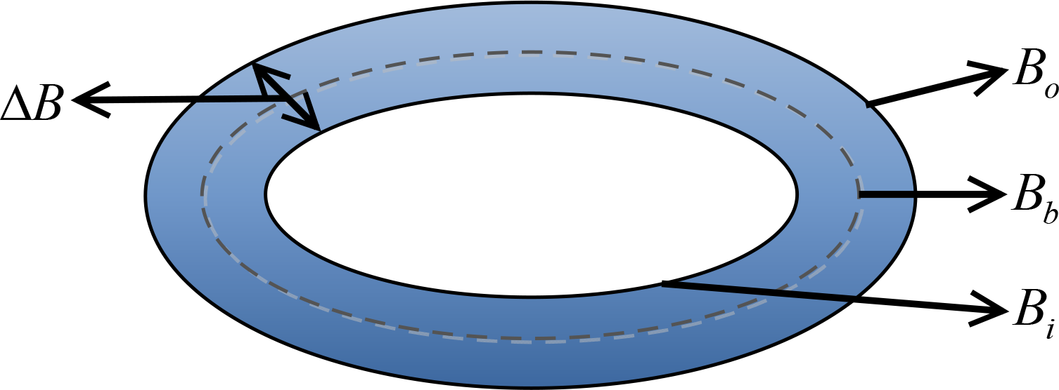
Let B_i and B_o represent two elliptical structuring elements with the same shape. As shown in Figure 5, B_o is called the outer structuring element. B_i is called the inner structuring element. B_b represents the structuring element whose size is between B_o and B_i. The margin structuring element ΔB= B_o − B_i is the margin region between B_i and B_o. The relationship of B_i, B_o, ΔB and B_b is demonstrated in Figure 5.

Operations f ■ B_oi and f □ B_oi are defined as follows:

$$f\blacksquare B_{\mathit{oi}}=\left(f\oplus \mathrm{\Delta }B\right)\ominus B_b$$

(9)

$$f\square B_{\mathit{oi}}=\left(f\ominus \mathrm{\Delta }B\right)\oplus B_b$$

(10)

where B_oi represents that the operation is related to B_o and B_i. Then, the new top-hat transformation can be defined as follows:

$$\text{NWTH}:NT=f-f\blacksquare B_{\mathit{oi}}$$

(11)

$$\text{NBTH}:\mathit{NB}=f\square B_{\mathit{oi}}-f$$

(12)

where NT is the image after the new WTH transformation (NWTH), and B is the image after new BTH transformation (NBTH). Furthermore, the new top-hat transformations use two correlated structuring elements, and the margin structuring element ΔB is used to utilize the difference information between vehicles and surrounding regions.

In NWTH, if the processed region is not a target region, the relationship of the pixels in the processed and surrounding regions is not confirmed. This indicates that there may be negative values in NWTH. To avoid this situation, NWTH can be modified as follows:

$$\text{NWTH}:\mathit{NT}(x,y)=max\left(f(x,y)-f(x,y)\right)\blacksquare B_{\mathit{oi}}(x,y),0)$$

(13)

Meanwhile, the modified NBTH can be defined as

$$\text{NBTH}:\hspace{0.17em}\mathit{NB}(x,y)\hspace{0.17em}\hspace{0.17em}=\hspace{0.17em}\hspace{0.17em}min\left(f(x,y)\right)\square B_{\mathit{oi}}(x,y)-f(x,y),0)$$

(14)

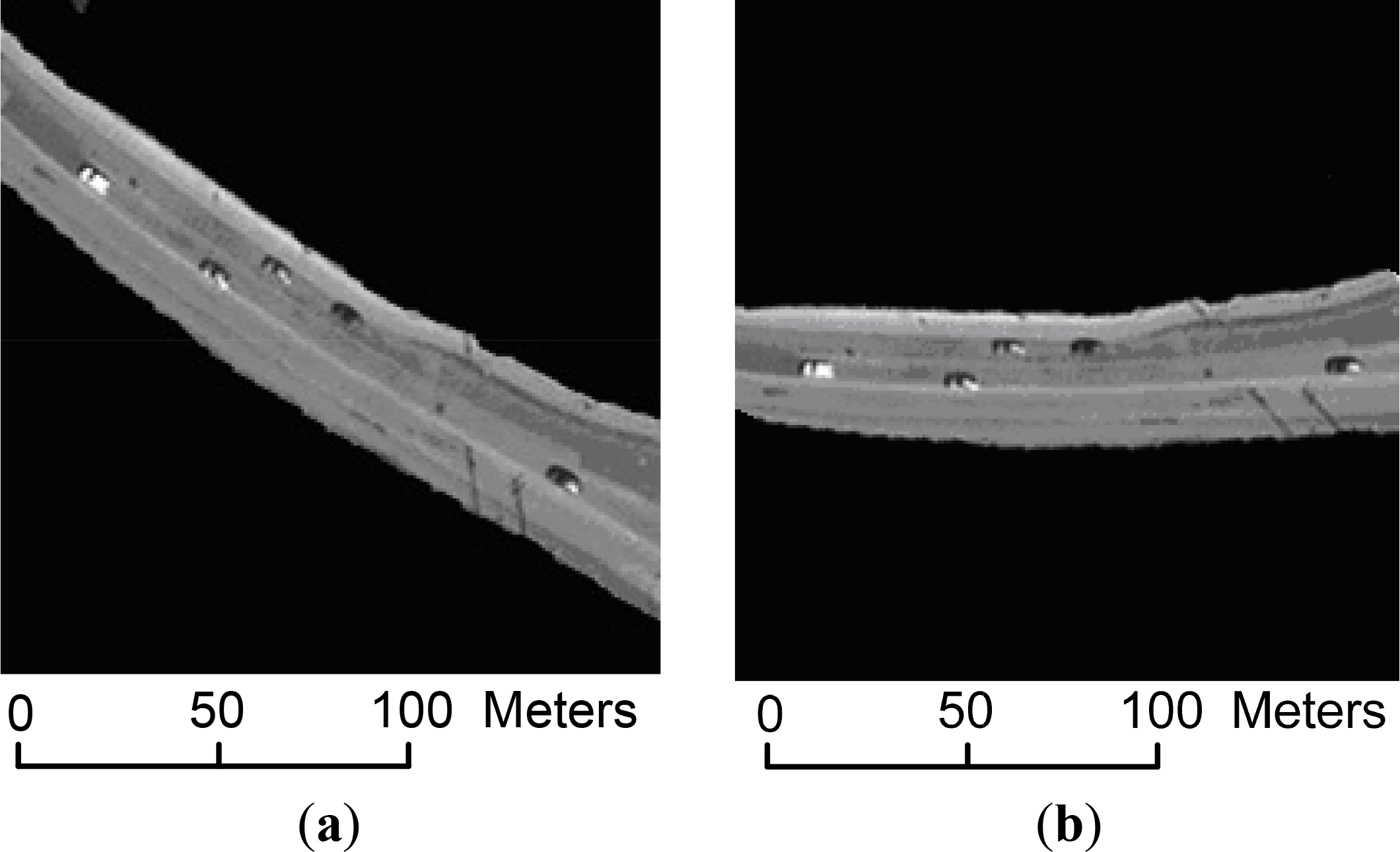
To apply the proposed method, the road is first divided into several smaller and partially overlapping sub-segments. Then, each sub-segment is rotated horizontally aligned, as shown in Figure 6. This step is essential, since the moving vehicles are oriented along the road. Thus, the vehicle’s elliptical structure can be better captured by NWTH and NBTH.

From a priori knowledge, in WorldView-2 images, the moving vehicles usually have a size of 6–10 pixels in length and 3–5 pixels in width. In this paper, ΔB represents the surrounding region of moving vehicles. B_b represents the vehicle region. To efficiently detect moving vehicles, the inner size of ΔB should be larger than the size of vehicles. To be efficient and robust, we set B_b with the size of 13 × 7, B_o with the size of 15 × 9 and B_i with the size of 11 × 5.

Furthermore, the vehicle candidate extraction method depends on its polarity. In Bar’s work [12], the notion of positive polarity means that a vehicle in the panchromatic image is brighter than the surrounding region, whereas negative polarity means that a vehicle in the panchromatic image is darker than the surrounding region. Since vehicles with positive polarity are relatively brighter than surrounding region, the NWTH operation extracts such vehicles. The NBTH operation extracts vehicles with negative polarity.

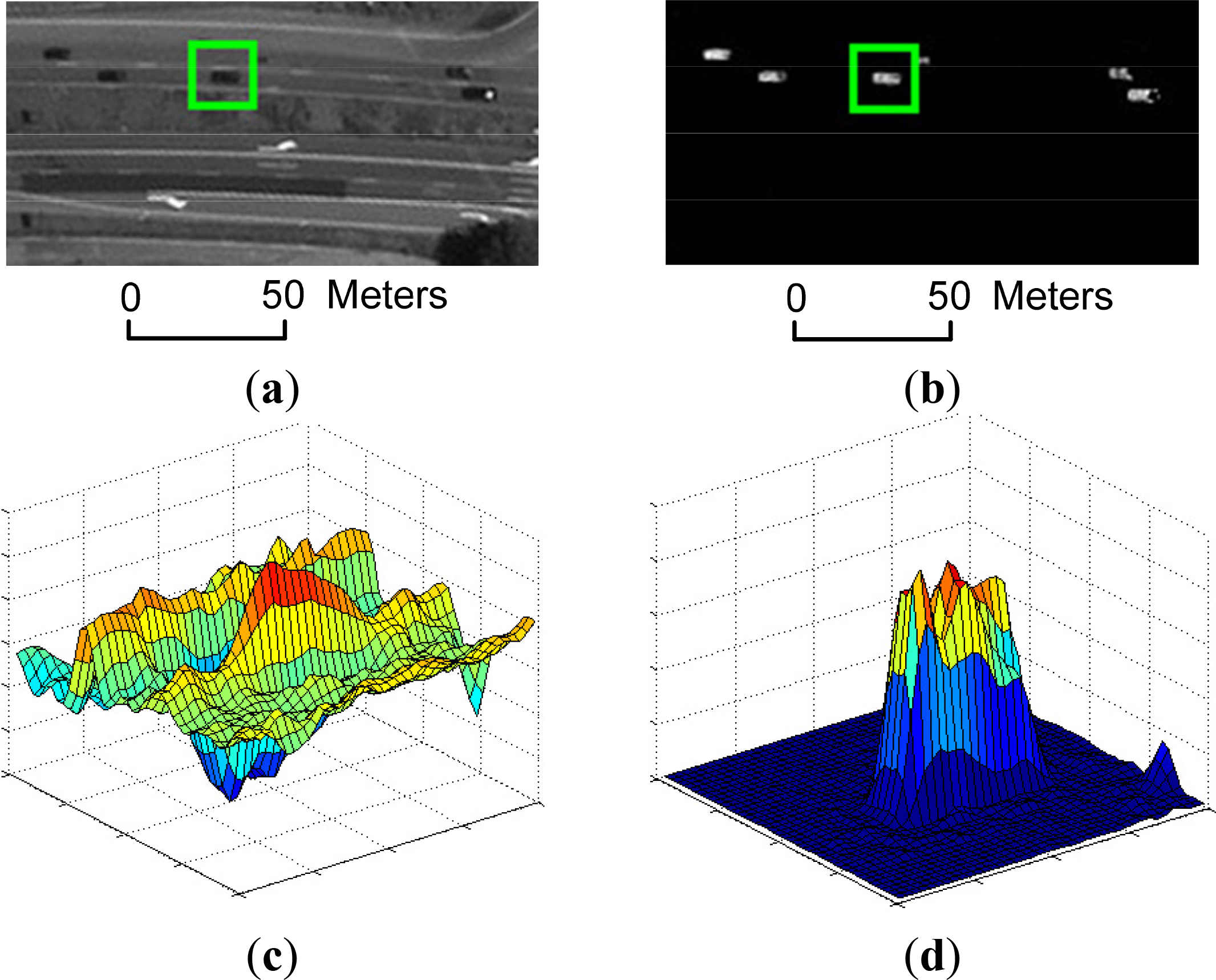
Examples of vehicle candidate location extraction results are shown in Figures 7 and 8. In both figures, (a) is the original image, (b) is the result image by the proposed method, (c) is the 3D distribution of the vehicle and surroundings in the square box in the original image and (d) is the 3D distribution of the vehicle and surroundings in the square box in the resulting image.

Figure 7 is an example of vehicles with positive polarity. After NWTH and NBTH, the cluttered backgrounds are well suppressed, and the vehicle region turns to bright spots. Figure 8 is the example of vehicles with negative polarity. After NWTH and NBTH, the noises and cluttered backgrounds are suppressed, and the vehicle regions are more clearly delineated.

2.3. Moving Vehicles Identification

After moving vehicle candidate extraction, there may be some false alarms in the result image, such as concrete road dividers, oil stains on the road, etc. Since some road dividers and oil stains have a similar appearance as vehicles, it is hard to effectively eliminate such false alarms by their appearance properties. Recent studies, however, observed the spatial displacement of moving targets in WV2 images [1,12], whereas stationary object do not have such properties. Hence, the spatial displacement is a reliable cue for moving vehicle identification.

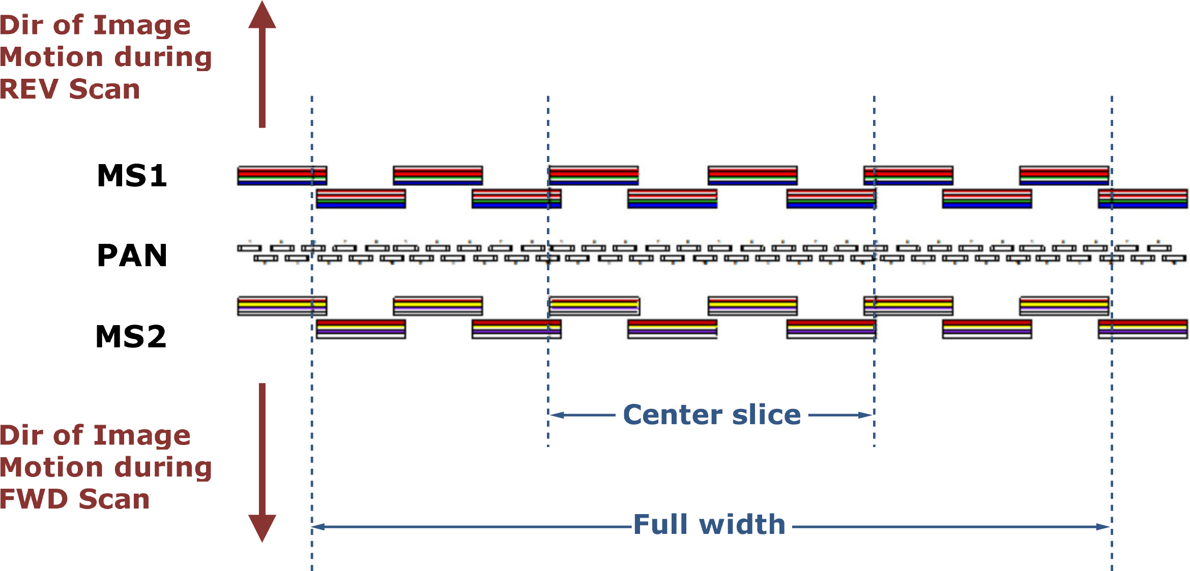
The WV2 satellite carries a PAN and two MS (MS1 and MS2) sensors onboard. The PAN sensor is located between the MS1 and MS2. MS1 consists of red, green, blue and NIR1. MS2 consists of red edge, yellow, coastal and NIR2. The focal plane layout of WV2 [18] is shown in Figure 9. Due to the hardware arrangement, the sequence of collected images is MS1, PAN and MS2 with approximately a 0.13-s time lag between each MS and the PAN image. Therefore, the time lag between MS1 and MS2 is approximately 0.26 s [1].

There are colorful fringes at moving targets in the WV2 fused image, which have been mostly treated as nuisance. That is because a moving target is observed at three different positions by the satellite, as shown in Figure 10. The dark and bright spots correspond to the dark and bright vehicles, respectively. The bright vehicle is moving toward the top of the image, while the dark vehicle is moving toward the bottom of the image.

Salehi et al. use standard PCA to detect moving vehicles [1]. Bar et al. proposed a method via spectral and spatial information (SNS) to identify moving vehicles [12]. In these methods, it is assumed that the influence of spectral difference between spectrally-neighboring bands is smaller than the temporal effect, and all eight spectral bands of WV2 are used to analyze moving vehicles. However, there may be big spectral differences between some spectrally-neighboring bands, and the spectral differences may influence the accuracy of moving vehicle identification. In this paper, we perform a band selection process by visual inspection and quantitative analysis, and three spectrally-neighboring band pairs are selected for moving vehicle identification. Furthermore, we propose the ERGAS-SNS method to identify moving vehicles. Through the analysis of the local ERGAS index, the dominant changed region could be extracted. Consequently, most of the spectral unchanged regions are eliminated, and the accuracy of moving vehicle identification is therefore improved.

2.3.1. Spectral Band Selection

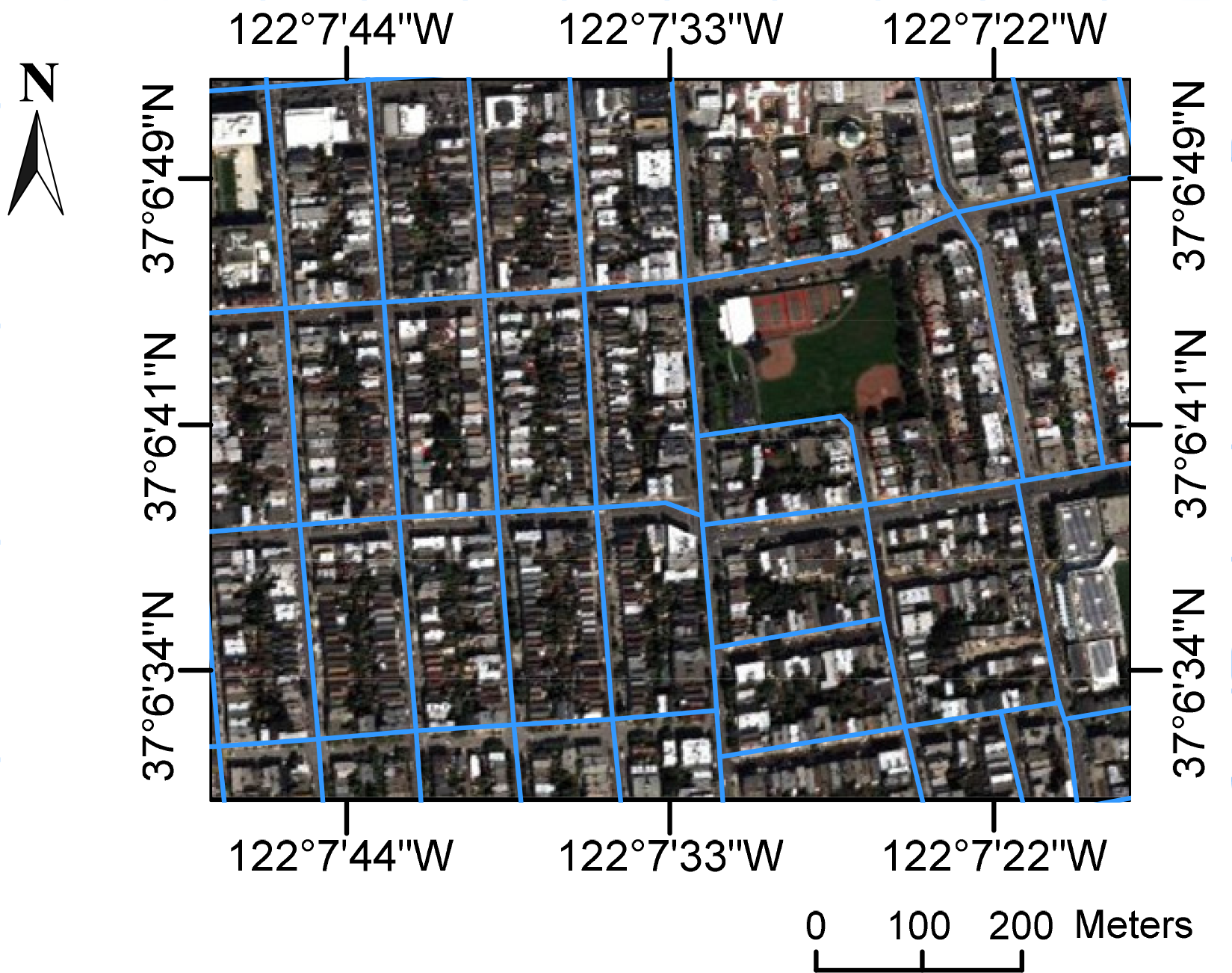
Ten clippings are randomly taken from the WV2 imagery of San Francisco for spectral band selection. Each of the clippings has a size of 500 × 500 pixels. We use the technique of image difference for visual inspection. The change detection maps between MS1 and MS2 spectral bands (C-B, Y-G, RE-R, NIR2-NIR1) are calculated. Sample change detection maps are shown in Figure 11. From (c–f), by visual inspection, we can see that there are dominant differences in the change detection map generated by RE-R. Furthermore, (g–j) show a regional enlarged image in red rectangles from (c–f), respectively. One moving vehicle locates in the center of the enlarge images. We could observe that in C-B, Y-G and NIR2-NIR1 maps, the vehicle is rather obvious. However, the vehicle in the RE-R map cannot be easily perceived, since heave background clutter is generated by the spectral differences.

Besides visual inspection, we performed the quantitative analysis by using root mean squared error (RMSE) analysis. RMSE is capable of measuring the global spectral distortion between two spectral bands. It exhibits a strong tendency to decrease when the spectral differences between the spectrally-neighboring bands decreases. As shown in Figure 12, the RMSE values of RE-R are dominantly high, whereas the RMSE values of other spectral band pairs are low. Based upon the above analysis, we conclude that the spectral band pair of RE-R is not suitable to identify moving vehicles.

From visual inspection and quantitative analysis, it can be derived that the spectrally-neighboring band pairs of C-B, Y-G and NIR2-NIR1 are beneficial for moving vehicle identification. Thus, we create new composite MS1 and MS2 images. The composite MS1 image consists of blue, green and NIR1. The composite MS2 image consists of coastal, yellow and NIR2. Both composite images are forwarded to the following ERGAS-SNS analysis.

2.3.2. ERGAS-SNS Analysis

Inspired by the SNS approach proposed by Bar [12], we investigate extending reliable change detection techniques for moving vehicle identification. The Erreur Relative Globale Adimensionnelle de Synthese (ERGAS) index proposed by Wald [19] is capable of measuring spectral difference between two spectral images. Following this insight, we incorporate ERGAS analysis into the SNS approach to detect the spatial displacement of moving vehicles.

The ERGAS index was originally designed to estimate the overall spectral quality of image fusion, and it is used to perform such a comparison:

$$\mathit{ERGAS}=100\frac{h}{l}\sqrt{\frac{1}{N}\sum _{k=1}^N{\left(\frac{\mathit{RMSE}(B_k)}{\mu (k)}\right)}^2}$$

(15)

where h and l denote the spatial resolutions of a high resolution image and a low resolution image, respectively. N is the number of spectral bands. k is the index of each band. RMSE(B_k) denotes the root mean square error for k-band between the fused image and the reference image. μ(k) denotes the mean of the k-band in the reference image. The index is capable of measuring spectra difference between two spectral images. Renza et al. [20] use the local ERGAS method for change detection. The new equation of local ERGAS is given by:

$$\mathit{ERGAS}\left(x,y\right)=100\sqrt{\frac{1}{N}\sum _{k=1}^N{\left(\frac{f_k\left(x,y\right)}{g_k}\right)}^2}$$

(16)

where the f_k (x,y) is the local RMSE and g_k is the mean of each spectral band.

Both images are first normalized to minimize the difference between them, and the local ERGAS method is applied to composite MS1 and MS2 images for local change detection. A window of a size of 5 × 5 scans every pixel of the candidate locations, and bright spots will be generated around moving vehicles. Figures 13 and 14 give example images given by local ERGAS analysis, where the values of the image are normalized to (0, 255). It can be seen that a moving vehicle turns into a pair of bright spots. The bright spots are forwarded to the SNS analysis.

In the SNS analysis [12], the change score is calculated between various spectral bands. In this paper, the change score (CS) is defined as:

$$CS\left(p\right)={\text{med}\left\{\text{M}1\left(p,b\right)-\text{M}2\left(p,b\right)\right\}}_{b=1\dots 3}$$

(17)

where med denotes the standard median operator, p is the pixel position, M1 denotes the composite MS1 band group (blue, green and NIR1) and M2 denotes the composite MS2 band group (coastal, yellow and NIR2). After change score calculation, the bright spot pair generated by ERGAS analysis would turn into a positive-negative pair in the change score map, as shown in Figures 13 and 14. This pair can be considered as a moving vehicle if and only if:

$$\begin{array}{c}\left(1\right)\hspace{0.17em}\hspace{0.17em}{p}_1\hspace{0.17em}\hspace{0.17em}\text{is}\hspace{0.17em}\text{a}\hspace{0.17em}\text{local}\hspace{0.17em}\text{maximum}\\ \left(2\right)\hspace{0.17em}\hspace{0.17em}{p}_2\hspace{0.17em}\hspace{0.17em}\text{is}\hspace{0.17em}\text{a}\hspace{0.17em}\text{local}\hspace{0.17em}\text{minimum}\\ \left(3\right)\hspace{0.17em}\hspace{0.17em}{D}_{min}<\Vert p_1,p_2\Vert <D_{max}\\ \left(4\right)\hspace{0.17em}\hspace{0.17em}{D}_{min}=min\left(L\right),\hspace{0.17em}\hspace{0.17em}{D}_{max}=max\left(L,D\right)\end{array}$$

(18)

where L is the vehicle’s length and D is the feasible displacement of the fastest moving object in the scene during the time gap. From a priori knowledge, vehicles in WV2 images often have a size of 6–10 pixels in length, and therefore, D_min is set to 6 pixels in our implementation. In addition, the general maximum speed of moving vehicles is about 160 km/h. It is about a 22-pixel displacement. Hence, D_max is set to 22 pixels in our implementation.

One moving vehicle generates a positive-negative pair (one bright spot and one dark spot) in ERGAS-SNS analysis. An interesting aspect of the positive-negative pair is that which spot belongs to MS1 or MS2 image depends on the vehicle’s polarity. If the vehicle is with positive polarity, the bright spot denotes the vehicles’ position in MS1 image, while the dark spot denotes the vehicles’ position in MS2 image. On the other hand, if the vehicle has negative polarity, the dark spot denotes the vehicle’s position in MS1 image, while the bright spot denotes the vehicle’s position in MS2 image. The phenomenon can be observed in Figure 13 and 14. As mentioned in Section 2.2, the NWTH operation extracts candidate locations of vehicles with positive polarity, and the NBTH operation extracts candidate locations of vehicles with negative polarity. Following this insight, the vehicle’s position in both MS1 and MS2 images can be extracted. Clearly, this is important information for moving vehicle speed and direction estimation.

2.4. Moving Information Extraction

The moving vehicle’s positions in MS1 and MS2 images can be extracted by ERGAS-SNS analysis, and the vehicle’s displacement can be calculated. The speed of a moving vehicle is determined by the displacement and time lag between MS1 and MS2. The displacement of moving vehicles in MS1 and MS2 is of sufficient precision, since the topography around the moving vehicles is changing smoothly, and road networks in general do not show very steep height gradients. Therefore, the speed of moving vehicles could be calculated by:

$$V=\frac{D}{\mathrm{\Delta }T}$$

(19)

where D is the displacement distance of moving vehicles and ΔT is the time lag between MS1 and MS2 (approximately 0.26 s). The minimum speed is defined by the resolution and the displacement during the time lag. In our observations, to have better results, the lower bound of speed is 40 km/h. This is equal to a 6-pixel displacement in 0.5-m resolution. Slower-moving vehicles are hard to accurately identify by the proposed method.

Due to the special focal plane assembly by WV2, during the small time lag, vehicles moves from the position in the MS1 image to the position in the MS2 image. Hence, the moving direction can be expressed by the azimuth. An azimuth of 0° implies a northward direction, and azimuth progression is calculated clockwise from north. For example, the bright car in Figure 10 moves downward, and its movement azimuth is 180°.

3. Experimental Results and Discussion

3.1. Study Area

The proposed method was applied to a WorldView-2 image covering San Francisco, California, in the USA. The image was collected at noon on Sunday, 9 October 2011. The image data is without snow or cloud cover and with sufficient lighting conditions to detect moving vehicles. Several scenes are taken for the demonstration of the proposed method, and these scenes are composed of urban roads and highways. The data is geo-rectified and radiometrically corrected. The RGB composition in the visible spectrum of the image is shown in Figure 15.

3.2. Overall Results and Discussion

As mentioned before, the overall goal is to develop a method for automatic monitoring the traffic conditions of suburban roads and highways by using WV2 images. Therefore, we perform the proposed method mainly on two types of roads: suburban roads and highways. Sixteen steer road segments containing 241 moving vehicles were analyzed. In these selected road segments, eight segments (1, 6, 7, 8, 9, 12, 15 and 16) are highways and eight segments (2, 3, 4, 5, 10, 11, 13 and 14) are suburban roads. The average width of highway segments is about 50 m, and the average width of suburban road segments is about 18 m. The average length of these segments is about 300 m.

We manually labeled the moving vehicles appearing in all road segments as the ground truth. Each MS1 and MS2 image pair is examined carefully, since some vehicles near the road intersections are not moving. In order to evaluate the results of various methods, a numerical accuracy assessment was conducted, and three statistical measures are chosen to exhibit the performance of detection methods:

$$\text{Correctness}=\frac{\text{TP}}{\text{TP}+\text{FP}}\times 100\%$$

(20)

$$\text{Completeness}=\frac{\text{TP}}{\text{TP}+\text{FN}}\times 100\%$$

(21)

$$\text{Quality}=\frac{\text{TP}}{\text{TP}+\text{FP}+\text{FN}}\times 100\%$$

(22)

where TP (true positive) denote the number of true detected moving vehicles, FP (false positive) is the number of false detected moving vehicles and FN (false negative) is the number of missed detections.

The correctness is a measure that indicates the detection accuracy rate relative to the ground truth. Correctness and completeness are the converse of commission and omission errors, respectively. The two measures are complementary and need to be interpreted simultaneously. The quality shows the overall accuracy of the method. The final detection results of moving vehicles of the proposed method are summarized in the

Table 1. Moving vehicle detection results of sixteen scenes. TP, true positive; FP, false positive; FN, false negative.

Scene	TP	FP	FN	Correctness (%)	Completeness (%)	Quality (%)
Scene 1	9	0	0	100.00	100.00	100.00
Scene 2	8	0	1	100.00	88.89	88.89
Scene 3	9	0	1	100.00	90.00	90.00
Scene 4	9	0	1	100.00	90.00	90.00
Scene 5	10	0	1	100.00	90.91	90.91
Scene 6	47	2	4	95.92	92.16	88.68
Scene 7	18	0	3	100.00	85.71	85.71
Scene 8	2	0	1	100.00	66.67	66.67
Scene 9	28	2	2	93.33	93.33	87.50
Scene 10	2	0	1	100.00	66.67	66.67
Scene 11	6	0	2	100.00	75.00	75.00
Scene 12	27	4	2	87.10	93.10	81.82
Scene 13	3	0	0	100.00	100.00	100.00
Scene 14	6	0	0	100.00	100.00	100.00
Scene 15	25	4	3	86.21	89.29	78.13
Scene 16	10	2	0	83.33	100.00	83.33
Total	219	14	22	93.99	90.87	85.88

.

We compared our method with several change detection techniques, so as to comprehensively analyze the performance of the proposed method. The change vector analysis (CVA) is a commonly used change detection technique for multispectral images [21]. Therefore, the CVA method has been implemented to detect moving vehicles. We also compare our method with the SNS method. Since we could not find the authors’ implementation, we implemented the SNS method in MALTAB.

Besides CVA, the image difference between two spectrally-neighboring bands is also used here. The change detection maps between the MS1 and MS2 spectral bands (C-B, Y-G, RE-R and NIR2-NIR1) are created. The moving vehicle detection results of these methods by using SNS analysis are summarized in

Table 2. Moving vehicle detection results of different techniques.

Method	TP	FP	FN	Correctness (%)	Completeness (%)	Quality (%)
C-B	150	7	91	95.54	62.24	60.48
Y-G	162	32	79	83.51	67.22	59.34
RE-R	113	11	128	91.13	46.89	44.84
NIR2-NIR1	166	30	75	84.69	68.88	61.25
CVA	181	17	60	91.41	75.10	70.16
SNS	209	27	32	88.56	86.72	77.99
ERGAS-SNS	219	14	22	93.99	90.87	85.88

.

As mentioned above, the quality measure shows the overall accuracy of the method. From Table 2, we can observe that the proposed method outperforms the other methods. Despite the relatively high correctness performance of the C-B method compared with the proposed method, many vehicles are missed, which decreases the overall performance of the C-B method. In addition, the RE-R method gets the lowest quality value. This is consistent with the result of band selection that the spectral band pair of RE-R is not suitable for moving vehicle identification. In the results of the SNS method, we observed that the some false alarms are generated due to the reason that there are big spectral differences between RE-R spectral band pair, and the spectral differences influence the detection accuracy. In the proposed method, a band selection process is performed, and the RE-R spectral band pair is excluded to reduce false alarms. Furthermore, in the SNS method, the positive-negative pairs are searched throughout the whole image. Hence, some false alarms are generated outside of the road, and some moving vehicles are missed due to the heavy clutter. In the proposed method, a road extraction procedure is employed, and this step reduces search areas and the number of false alarms. Local ERGAS analysis is employed to identify moving vehicles, and moving vehicles turn into a pair of bright spots. The special feature can greatly reduce the exhaustive burden of SNS analysis.

Scene 9 presents part of a highway, and the detection results of the scene are shown in Figure 16. Thirty moving vehicles are detected, including two false alarms. Two vehicles are observed as missed detections, and they are referred to as false negatives. The two false alarms obtained are generated by the vehicles’ shadows. The reason for missed vehicles is due to the fact that the vehicles with negative polarity adhere to building shadows, causing them to be removed as shadow regions.

Scene 2 presents part of some suburban roads. As can be seen from Figure 17, no false alarms were found, while one vehicle is missed. The missed car is close to another car, and the two cars’ hypothesis points unite together. Thus, insufficient image resolution influences the accuracy of vehicle detection.

In all of the road segments, 22 moving vehicles were missed. One reason for the misses is the fact that shadows of trees and buildings tend to hide vehicles. As shown in Figure 18 (part of the enlarged image from Scene 9), one vehicle was passing under building shadows, and the negative-positive pair feature could not be detected. The second reason for the missed detection is the fact that some vehicles’ spectral values are very close to the road. As shown in Figure 19, one vehicle moves upwards. However, the vehicle has similar spectral values with the road, and then, the vehicle is hard to perceive. In addition, as mentioned above, insufficient image resolution also causes some misdetections.

3.3. Moving Vehicle Information Extraction Results and Discussion

We estimate the speed and direction of the detected vehicles by using the method described in Section 2.4. Part of the enlarged version from Scene 9 (Highway) is shown in Figure 20. Meanwhile, part of the enlarged version from Scene 14 (suburban road) is shown in Figure 21. The corresponding vehicle speed histograms are presented, and the movement directions of vehicles are labeled.

As can be observed, vehicles in Scene 14 move slower than vehicles in Scene 9. This is due to the simple reason that the speed limit of suburban roads is lower than the highway. Vehicle 10 is running at 79 km/h, while Vehicles 11 and 12 have slower speeds (67 and 71 km/h, respectively). This is mainly because Vehicles 11 and 12 just passed one curve of the road.

The speed estimation results of 166 moving vehicles for highway segments are as shown in Figure 22. The max speed of these vehicles is about 142 km/h, and these vehicles have an average speed of 99 km/h. Meanwhile, the speed estimation results of 53 moving vehicles for suburban roads are as shown in Figure 23. These vehicles have an average speed of 70 km/h. This means that vehicles on highways run faster than vehicles on suburban roads. The results show that the speed estimation results are in accordance with actual conditions.

4. Conclusions

In this paper, we have developed a method to monitor the traffic conditions of suburban road and highways by using WV2 images, and a novel method was proposed for moving vehicle detection and speed estimation by exploiting the special focal plane assembly by WV2. An improved top-hat transformation based on the vehicles’ appearance properties is utilized to extract vehicle candidate locations. Meanwhile, an ERGAS-SNS analysis is proposed to identify moving vehicles. Finally, the speeds of vehicles are estimated by calculating the displacements between MS1 and MS2 images. The experimental results show the good performance of the proposed method. The proposed method is a promising tool for traffic monitoring by using satellite images.

Road extraction is a crucial process of moving vehicle detection. In real applications, a frequent problem is that parts of the image may be covered by clouds. This makes moving vehicle detection more challenging. Hence, in our future work, a cloud mask would be used to handle cloud-contaminated images. On the other hand, it is very interesting to use more band pairs for moving vehicle detection, e.g., Red-PAN, NIR2-PAN. Our future work will take these band pairs into account.

We recognize that there is still potential for accuracy improvement in speed estimation. In order to improve the accuracy of speed estimation results, the exact time lag between the acquisition of the MS1 and MS2 images has to be known. Furthermore, DigitalGlobe plans to launch WorldView-3, providing 0.31-m panchromatic resolution. Such a resolution can increase the accuracy of the vehicles’ centroid extraction. Our future research will focus on how to enhance the accuracy of speed estimation.

References

1. Salehi, B.; Zhang, Y.; Zhong, M. Automatic moving vehicles information extraction from single-pass WorldView-2 imagery. IEEE J. Sel. Topics Appl. Earth Observ. Remote Sens 2012, 5, 135–145. [Google Scholar]
2. Zhang, Y.; Xiong, Z. Moving vehicle detection using a single set of QuickBird imagery–An initial study. In Proceedings of the ISPRS Commission VII Mid-Term Symposium “Remote Sensing: From Pixels to Processes”, Enschede, The Netherlands, 8–11 May 2006; pp. 397–402.
3. Tuermer, S.; Leitloff, J.; Reinartz, P.; Stilla, U. Evaluation of selected features for car detection in aerial images. In Proceedings of the ISPRS Hannover Workshop, High-Resolution Earth Imaging for Geospatial Information, Hannover, Germany, 14–17 June 2011; pp. 341–346.
4. Kembhavi, A.; Harwood, D.; Davis, L.S. Vehicle detection using partial least squares. IEEE Trans. Pattern Anal. Mach. Intell 2011, 33, 1250–1265. [Google Scholar]
5. Zheng, Z.; Zhou, G.; Wang, Y.; Liu, Y.; Li, X.; Wang, X.; Jiang, L. A novel vehicle detection method with high resolution highway aerial image. IEEE J. Sel. Topics Appl. Earth Observ. Remote Sens 2013, 6, 2338–2343. [Google Scholar]
6. Leitloff, J.; Hinz, S.; Stilla, U. Vehicle detection in very high resolution satellite images of city areas. IEEE Trans. Geosci. Remote Sens 2010, 48, 2795–2806. [Google Scholar]
7. Larsen, S.Ø.; Salberg, A.B.; Eikvil, L. Automatic system for operational traffic monitoring using very-high-resolution satellite imagery. Int. J. Remote Sens 2013, 34, 4850–4870. [Google Scholar]
8. Eikvil, L.; Aurdal, L.; Koren, H. Classification-based vehicle detection in high-resolution satellite images. ISPRS J. Photogramm. Remote Sens 2009, 64, 65–72. [Google Scholar]
9. Easson, G.; DeLozier, S.; Momm, H.G. Estimating speed and direction of small dynamic targets through optical satellite imaging. Remote Sens 2010, 2, 1331–1347. [Google Scholar]
10. Liu, W.; Yamazaki, F.; Vu, T.T. Automatic vehicle extraction and speed determination from QuickBird satellite images. IEEE J. Sel. Topics Appl. Earth Observ. Remote Sens 2011, 4, 75–82. [Google Scholar]
11. Krauß, T.; Stätter, R.; Philipp, R.; Bräuninger, S. Traffic flow estimation from single satellite images. In Proceedings of the SMPR Conference ISPRS Archives, XL-1/W (WG I/4), Tehran, Iran, 5–8 October 2013; pp. 241–246.
12. Bar, D.; Raboy, S. Moving car detection and spectral restoration in a single satellite WorldView-2 imagery. IEEE J. Sel. Topics Appl. Earth Observ. Remote Sens 2013, 6, 2077–2087. [Google Scholar]
13. Otsu, N. A threshold selection method from gray-level histograms. IEEE Trans. Syst. Man. Cybern 1979, 9, 62–69. [Google Scholar]
14. Chung, K.; Lin, Y.; Huang, Y. Efficient shadow detection of color aerial images based on successive thresholding scheme. IEEE Trans. Geosci. Remote Sens 2009, 47, 671–682. [Google Scholar]
15. Alcantarilla, P.F.; Bartoli, A.; Davison, A.J. KAZE features. In Proceedings of the European Conference on Computer Vision (ECCV), Fiorenze, Italy, 7–13 October 2012; pp. 214–227.
16. Perona, P.; Malik, J. Scale-space and edge detection using annisotropic diffusion. IEEE Trans. Patt. Anal. Mach. Intell 1990, 12, 629–639. [Google Scholar]
17. Bai, X.; Zhou, F. Analysis of new top-hat transformation and the application for infrared dim small target detection. Patt. Recogn 2010, 43, 2145–2156. [Google Scholar]
18. Updike, T.; Comp, C. Radiomtric Use of WorldView-2 Imagery. Available online: http://www.digitalglobe.com/downloads/Radiometric_Use_of_WorldView-2_Imagery.pdf (accessed on 23 February 2014).
19. Wald, L. Data Fusion: Definitions and Architectures: Fusion of Images of Different Spatial Resolutions; Presses des MINES: Paris, France, 2002. [Google Scholar]
20. Renza, D.; Martinez, E.; Arquero, A. A new approach to change detection in multispectral images by means of ERGAS index. IEEE Geosci. Remote Sens. Lett 2013, 10, 76–80. [Google Scholar]
21. Chen, J.; Chen, X.H.; Cui, X.H.; Chen, J. Change vector analysis in posterior probability space: A new method for land cover change detection. IEEE Geosci. Remote Sens. Lett 2012, 8, 317–321. [Google Scholar]
Figure 1. Flow diagram of the proposed method.
Remotesensing 06 06500f1
Figure 2. Image-to-vector geo-referencing of WorldView-2 imagery. This is one part of the Richmond District. The blue lines represent the road network.
Remotesensing 06 06500f2
Figure 3. Flow diagram of the road extraction.
Remotesensing 06 06500f3
Figure 4. Result of PAN image enhancement: (a) regional portion of highway; (b) enhanced image of (a); (c) regional portion of suburban road; (d) enhanced image of (c).
Remotesensing 06 06500f4
Figure 5. Relationship of the structuring elements.
Remotesensing 06 06500f5
Figure 6. Road segment rotation: (a) original road sub-segment; (b) rotated road sub-segment.
Remotesensing 06 06500f6
Figure 7. Vehicle (positive polarity) extraction results: (a) original image; (b) candidate location; (c) 3D distribution of vehicle and surroundings in the original image; (d) 3D distribution of vehicle and surroundings in the resulting image.
Remotesensing 06 06500f7
Figure 8. Vehicle (negative polarity) extraction results: (a) original image; (b) candidate location; (c) 3D distribution of vehicle and surroundings in the original image; (d) 3D distribution of the vehicle and surroundings in the resulting image.
Remotesensing 06 06500f8
Figure 9. The focal plane layout of WorldView-2.
Remotesensing 06 06500f9
Figure 10. Regional enlarged image of moving vehicles: bright vehicle in the MS1 image (a); in the PAN image (b) and in the MS2 image (c); dark vehicle in the MS1 image (d); in the PAN image (e) and in the MS2 image (f).
Remotesensing 06 06500f10
Figure 11. Change detection maps between spectrally-neighboring bands: (a) MS1 image; (b) MS2 image; (c) C-B; (d) Y-G; (e) RE-R; (f) NIR2-NIR1, (g) C-B; (h) Y-G; (i) RE-R; (j) NIR2-NIR1.
Remotesensing 06 06500f11
Figure 12. Quantitative analysis of spectral differences of the WorldView-2 image.
Remotesensing 06 06500f12
Figure 13. ERGAS-SNS analysis of a bright vehicle: (a) composite MS1 image; (b) composite MS2 image; (c) ERGAS result; (d) SNS result.
Remotesensing 06 06500f13
Figure 14. ERGAS-SNS analysis of a dark vehicle: (a) composite MS1 image; (b) composite MS2 image; (c) ERGAS result; (d) SNS result.
Remotesensing 06 06500f14
Figure 15. RGB composition in the visible spectrum of Worldview-2 image covering San Francisco, CA, USA.
Remotesensing 06 06500f15
Figure 16. Moving vehicle detection results of Scene 9.
Remotesensing 06 06500f16
Figure 17. Moving vehicle detection results of Scene 2.
Remotesensing 06 06500f17
Figure 18. A vehicle passing under building shadows: (a) MS1 image; (b) MS2 image.
Remotesensing 06 06500f18
Figure 19. A vehicle has a similar spectral value to the road: (a) MS1 image; (b) MS2 image.
Remotesensing 06 06500f19
Figure 20. Results of moving vehicles’ speed and direction estimation: (a) vehicles on a highway labeled with movement directions; (b) speed estimation results.
Remotesensing 06 06500f20
Figure 21. The results of moving vehicles’ speed and direction estimation: (a) vehicles on a suburban road labeled with movement directions; (b) speed estimation results.
Remotesensing 06 06500f21
Figure 22. Speed estimation results of 166 moving vehicles on highways.
Remotesensing 06 06500f22
Figure 23. Speed estimation results of 53 moving vehicles on suburban roads.
Remotesensing 06 06500f23