1982–2010 Trends of Light Use Efficiency and Inherent Water Use Efficiency in African vegetation: Sensitivity to Climate and Atmospheric CO2 Concentrations

 ,
,
Abstract
: Light and water use by vegetation at the ecosystem level, are key components for understanding the carbon and water cycles particularly in regions with high climate variability and dry climates such as Africa. The objective of this study is to examine recent trends over the last 30 years in Light Use Efficiency (LUE) and inherent Water Use Efficiency (iWUE*) for the major biomes of Africa, including their sensitivities to climate and CO2. LUE and iWUE* trends are analyzed using a combination of NOAA-AVHRR NDVI3g and fAPAR3g, and a data-driven model of monthly evapotranspiration and Gross Primary Productivity (based on flux tower measurements and remote sensing fAPAR, yet with no flux tower data in Africa) and the ORCHIDEE (ORganizing Carbon and Hydrology In Dynamic EcosystEms) process-based land surface model driven by variable CO2 and two different gridded climate fields. The iWUE* data product increases by 10%–20% per decade during the 1982–2010 period over the northern savannas (due to positive trend of vegetation productivity) and the central African forest (due to positive trend of vapor pressure deficit). In contrast to the iWUE*, the LUE trends are not statistically significant. The process-based model simulations only show a positive linear trend in iWUE* and LUE over the central African forest. Additionally, factorial model simulations were conducted to attribute trends in iWUE and LUE to climate change and rising CO2 concentrations. We found that the increase of atmospheric CO2 by 52.8 ppm during the period of study explains 30%–50% of the increase in iWUE* and >90% of the LUE trend over the central African forest. The modeled iWUE* trend exhibits a high sensitivity to the climate forcing and environmental conditions, whereas the LUE trend has a smaller sensitivity to the selected climate forcing.
1. Introduction
Terrestrial gross primary productivity (GPP) and evapotranspiration (ET), two critical components of the terrestrial carbon and water cycles, are driven by solar radiation and limited by soil moisture (and nutrient) availability [1–7]. In Africa where 50% of the land areas are covered by arid and semi-arid ecosystems [8], the limiting factors of GPP and ET include precipitation, which controls soil moisture available for plants, and nutrient availability [9–13]. Here, we investigate two widely used vegetation resource use variables, which offer valuable insight into the representation of carbon and water coupling in ecosystem process models: Light Use Efficiency (LUE) and inherent Water Use Efficiency at the ecosystem level (iWUE*).LUE is defined as the ability of the vegetation to use GPP per unit of Absorbed Photosynthetically Active Radiation (APAR) that is limited by temperature and water shortage [14,15]. This definition integrates limiting environmental factors through the fraction of absorbed photosynthetically active radiation (fAPAR) and provides LUE value below its theoretical potential value used in several studies [1,16,17].
iWUE* is defined as the product of GPP and vapor pressure deficit (VPD) per ET unit [18]. Because of the strong relationship between VPD and stomatal conductance [19,20], iWUE* appears to be more relevant than the water use efficiency to describe the biochemical functions of plants at ecosystem level [18]. The dependence of iWUE* on environmental conditions indicates possible adaptive adjustment of ecosystem physiology in response to a changing environment.
African ecosystems, especially the northern savannah, experienced a highly variable climate during the last decades, which directly affects pan-tropical climate and ecosystem water and carbon fluxes [21–26]. Previous studies reported that high climate variability in terms of solar incidence (through cloudiness), rainfall, temperature and VPD impacts LUE and iWUE* [27–29]. Atmospheric CO2 and land use change also alter ecosystem physiology and structure, and consequently LUE and iWUE* trends [30–34].
Because of the scarcity and heterogeneity spatial distribution of existing in situ measurements in Africa [35,36], remote sensing products are valuable to constrain phenology and carbon fluxes over Africa, and were used in several previous studies [37–39]. Two satellite-based long-term records are used in this study to assess and analyze iWUE* and LUE simulated by different versions of the ORCHIDEE (ORganizing Carbon and Hydrology In Dynamic EcosystEms) land surface model. The 1982–2010 fAPAR3g third generation satellite dataset is used to generate the LUE data product [40]. 1982–2010 GPP and ET data products were generated from an empirical model calibrated from in situ measurements at FLUXNET sites and are used in LUE and iWUE* calculation [41]. The VPD and PAR (photosynthetic active radiation), needed for the calculation of iWUE* and LUE respectively, are computed using the WATCH-Forcing-Data-ERA-Interim (WFDEI) climate reanalysis.
The main goal of this present study is to assess the LUE and iWUE* trends during 1982–2010 using the remote sensing product and to evaluate the ability of ORCHIDEE to better reproduce these trends of vegetation resource use. Furthermore, we separate the CO2 and climate effects on LUE and iWUE* trends by using factorial simulations: (1) a simulation with a constant CO2 and (2) a simulation with an alternative climate forcing.
2. Materials and Methods
2.1. Model Description
The ORCHIDEE land surface model deals with carbon, water and energy exchanges between the atmosphere and biosphere [42]. The vegetation is defined as a mosaic of 12 plant functional types (PFTs) based on morphology (tree or grass), leaf type (needle-leaf or broad-leaf), phenology (evergreen, summer-green or rain-green), photosynthetic pathway for crops and grasses (C3 and C4) and climatic regions (boreal, temperate and tropical). African vegetation includes 7 PFTs: C3 and C4 grass, C3 and C4 agriculture, evergreen and rain-green tropical broadleaved and temperate broadleaved evergreen trees. The GPP function that describes carbon assimilation, is based on the leaf scale equations for C3 and C4 PFTs from Farquhar and Collatz respectively [43,44]. The scaling of GPP per layer within the canopy assumes an exponential attenuation of light following a big-leaf approximation. The foliage density (LAI) and plant water stress are prognostic and can impact GPP, carbon allocation, leaf age and senescence [42]. The variable fAPAR can be diagnosed from LAI output using the Ruimy formulation [45]: fAPAR = 0.95 × (1 − exp(−0.5 × LAI)).
The energy exchanges (transport of radiation and heat) and water balance between the vegetation-soil-atmosphere are described in [46,47]. Total ET is the sum of five components including evaporation of water intercepted by the canopy, transpiration by the vegetation and bare soil evaporation. The two other components of total ET in ORCHIDEE are snow sublimation (negligible in Africa) and evaporation from floodplains (river routing and floodplain hydrology scheme is not activated in this study). To simplify the transpiration parameterization, as well as for photosynthesis and light competition, ORCHIDEE does not account for fluxes from, and competition with, understory vegetation [42]. Bare soil evaporation is controlled by soil moisture and, thus, depends on the soil hydrology parameterization of ORCHIDEE. Transpiration is governed by the ability of the roots to extract water from the soil, assuming a PFT-dependent exponential root profile [47]. Simulated water stress from soil moisture availability influences photosynthesis and stomatal conductance through a scaling factor that is associated with relative soil moisture when the root zone relative soil moisture, i.e., volumetric soil moisture normalized by the difference between field capacity and wilting point, falls below a threshold value [48].
The default ORCHIDEE hydrological scheme (hereafter, the two-layer version) is based on a simple two-layer bucket-type model [46]. The soil upper layer varies according to the water availability, and the deep soil layer is filled from top to bottom with precipitation. When ET is larger than precipitation, water is removed from the upper layer until it dries out, leaving only the deep soil layer. To analyze the role of a more realistic soil hydrology scheme on LUE and iWUE* trends (i.e., fAPAR, GPP and ET), we also use a second version of ORCHIDEE model with a soil diffusion model of 11 layers [49–51]. The 11-layer soil scheme represents a vertical soil flow based on physical processes from the Fokker-Planck equation that resolves water diffusion in non-saturated conditions from the Richards equation [52]. The soil physics in the 11-layer version is based on the CWRR (Center for Water Resources Research) model [53,54]. The vertical discretization is not uniform: the grid being finer near the surface (the 3 topmost layers being 1 centimeter apart) where the soil moisture mostly varies, in order to represent the rapid exchanges of soil moisture near the surface [49]. Note that, in this study, the soil depth is uniformly fixed at 2m for both ORCHIDEE versions.
2.2. Climate Forcing
Daily meteorological fields used to drive ORCHIDEE are from the recent WFDEI reanalysis (1979–2010 period) that consists of bias corrected ERA-Interim fields with a bias correction for precipitation using GPCCv5 rain gauge measurements[55–57]. WFDEI is computed at 0.5° spatial resolution and is also used in the calculation of the incident photosynthetically active radiation (PAR) and VPD. The LUE and iWUE* sensitivity to climate forcing is estimated by driving ORCHIDEE with another climate forcing called WFD. WFD is the 20th century WATCH Forcing Data based on ERA40 (1958–2001), and extended back to 1901 [58]. The WFD precipitation is bias corrected using the GPCCv4 rain gauge measurements instead of GPCCv5 for WFDEI. Since WFD stops in 2001, we extend this forcing by using ERA-Interim data during 2001–2010.
2.3. Simulations
Between 200 and 300 years of spin-up are required to reach equilibrium in the biomass carbon pools over African ecosystems before running ORCHIDEE simulations [59]. The spin-up run repeatedly uses climate forcing data of the 1979–1988 period at 0.5° spatial resolution with atmospheric CO2 concentration fixed at the value of year 1979 (336.5 ppm). Four factorial simulations (Table 1) are conducted, starting from spin-up derived equilibrium state. Simulation S1 uses the 11-layer soil diffusion scheme, WFDEI climate and transient atmospheric CO2. S2 simulation uses the simpler 2-layer ORCHIDEE version and is otherwise identical to S1. The effect of increasing atmospheric CO2 on LUE and iWUE* trends is analyzed with the S2-FIXCO2 simulation, identical to S2 except for a fixed atmospheric CO2 value (336.5 ppm as of 1979). The sensitivity of LUE and iWUE* to input climate forcing data is investigated by comparing S2-WFD driven by WFD with S2.
2.4. Datasets for Model Evaluation
To generate LUE and iWUE* data products, we used the GIMMS fAPAR3g and the model tree ensemble (MTE) products (MTE-GPP and MTE-ET) [40,41].
2.4.1. fAPAR3g
The Global Inventory Modeling and Mapping Studies third generation GIMMS fAPAR3g product is used to calculate the Absorbed Photosynthetically Active Radiation (APAR). The fAPAR3g GIMMS satellite data is based on Normalized Difference Vegetation Index data (GIMMS NDVI3g [40]), derived from the Advanced Very High Resolution Radiometers (AVHRR) aboard a series of US National Oceanic and Atmospheric Administration (NOAA) satellites. The spatial-temporal resolution of the dataset is 8 km and has a 15-day time step. The original 8-km fAPAR3g data are re-aggregated to the ORCHIDEE resolution of 0.5° using bilinear interpolation.
2.4.2. MTE Product
The 0.5° gridded GPP and ET from MTE data-driven model are used to calculate LUE and iWUE* [41]. The data-driven model integrates site-level flux tower measurements of GPP and ET fluxes to global scale using the statistical approach of MTE. The MTE approach is based on a combination of TRee Induction ALgorithm (TRIAL) and Evolving tRees with RandOm gRowth (ERROR) technique [37]. The trained MTE at site level is used to generate global GPP (MTE-GPP) and ET fluxes (MTE-ET) [41]. The estimation of MTE-GPP and MTE-ET from extrapolation of local FLUXNET measurements is based on 29 explanatory variables, including precipitation and temperature (both measured in situ) and remote sensing indices of monthly fAPAR from GIMMS during the 1982–1997 period, SeaWiFs sensor during 1998–2005, and MERIS since 2006 [41]. Because the MTE data-driven model integrates several measurements, it is taken as a reference to evaluate the ORCHIDEE results. Note that the fAPAR3g (15-day resolution) and MTE products (monthly resolution) are available from 1982 to 2010.
2.5. LUE and iWUE* Calculation
2.5.1. LUE
The calculation of LUE is based on the widely used formulation [14,60]:
2.5.2. iWUE*
At ecosystem level, monthly iWUE* is calculated following the formulation [18]:
Note that, as for data products, the ORCHIDEE modeled iWUE* and LUE are obtained from the GPP, fAPAR and ET outputs variables at monthly time scale. The VPD and PAR are directly calculated from the climate inputs.
2.6. Trend Analysis
Trends are calculated by fitting linear functions for time series of annual LUE and iWUE* for each pixel using ordinary least-squares regression (OLS). Trends are computed with 95% confidence interval (here after 95% CI) using the Student’s t-test. The t-test compares a calculated t with a critical tc value for a stipulated significance level and N-2 degrees of freedom (N = 29; representing here the annual time series length: 1982–2010). No significant trends (|t| < tc) at 95% CI) are labeled in maps with grey and slate grey colors for negative and positive trends respectively. Trends for fAPAR, GPP and ET during 1982–2010 are also calculated from annual values following the same method as for LUE and iWUE*. All trends are weighted by their average over the whole period in order to compute the result in “%” of each parameter.
3. Results
3.1. Evaluation of ORCHIDEE iWUE* and LUE Average
3.1.1. Average iWUE* during 1982–2010
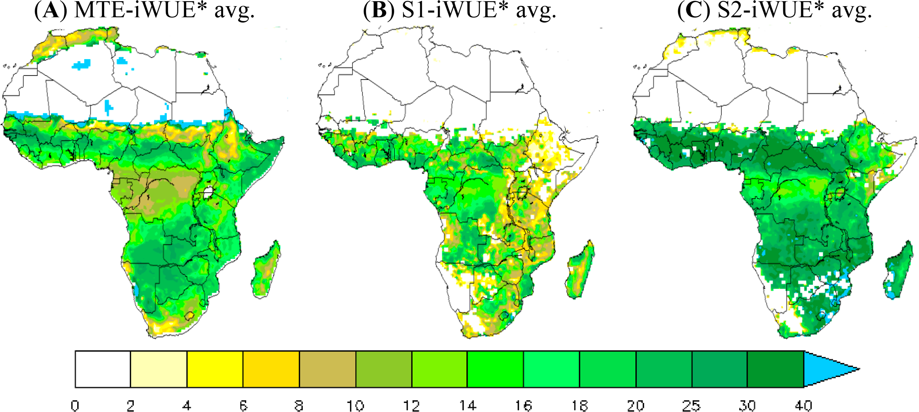
Figure 1 shows the multi-year averaged iWUE* during 1982–2010. High values of iWUE* from the MTE product are found over savannahs and rain-green woodland areas (northern savannahs and the southern edge of African central forests). The average MTE-iWUE* over these regions is 18 gC·hPa·mm−1·m−2. The maximum MTE-iWUE* value reaches up to 30 gC·hPa·mm−1·m−2 in the southern edge of the central African forest and more than 35 gC·hPa·mm−1·m−2 in some grid cells over the northern savannahs. In contrast, lower MTE-iWUE* values are found in the central African forest with values of less than 12 gC·hPa·mm−1·m−2 (the vapor pressure deficit is low in the central African forest).
The ORCHIDEE 11-layer version significantly underestimates iWUE* over the grasslands and savannah zones in comparison with the MTE product derived iWUE* (iWUE*< 20 gC·hPa·mm−1·m−2 over a large part of Africa). In contrast, the iWUE* from the 11-layer run is higher than the MTE-iWUE* over the central African forest (15 gC·hPa·mm−1·m−2 vs. 10 gC·hPa·mm−1·m−2). Unlike the 11-layer version, the 2-layer version overestimates iWUE* over the whole continent, especially over the grasslands and savannah zones (iWUE* ≈ 28 gC·hPa·mm−1·m−2 against 15 gC·hPa·mm−1·m−2 vs. 18 gC·hPa·mm−1·m−2 for MTE-iWUE* averaged in grassland areas).
Note that the difficulty of ORCHIDEE to reproduce the high iWUE* of arid and desert transition zones is probably due to problems in the land cover map used in this study and to the lack of a shrub-land PFT in the ORCHIDEE model [47,63].
3.1.2. Average LUE during 1982–2010
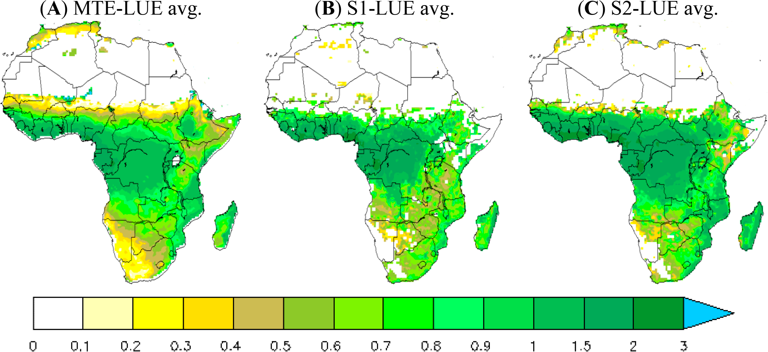
The spatial pattern of LUE is similar to that of GPP (data not shown). Maximum LUE values are found in the central African forest where the PAR is lower (because of clouds), whereas low LUE values are observed in Sahelian and African southern zones where PAR is high. The MTE-LUE average over grasslands and savannas is less than 0.7 gC·MJ−1·APAR, with a maximum value of 2.5 gC·MJ−1·APAR in some grid cells. In the central African forest, average MTE-LUE reaches up to 1.3 gC·MJ−1·APAR (maximum value 2.6 gC·MJ−1·APAR). The ORCHIDEE-simulated LUE matches the MTE-LUE better in the 11-layer version than the 2-layer version. The later overestimates LUE across the entire continent (Figure 2C). Taking grasslands as an example, the 11-layer version estimates LUE around 0.73 gC·MJ−1·APAR against 0.9 gC·MJ−1·APAR for the 2-layer, and 0.7 gC·MJ−1·APAR for the MTE-LUE.
3.2. iWUE* and LUE Trend during 1982–2010
3.2.1. iWUE* Trend during 1982–2010
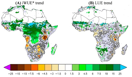
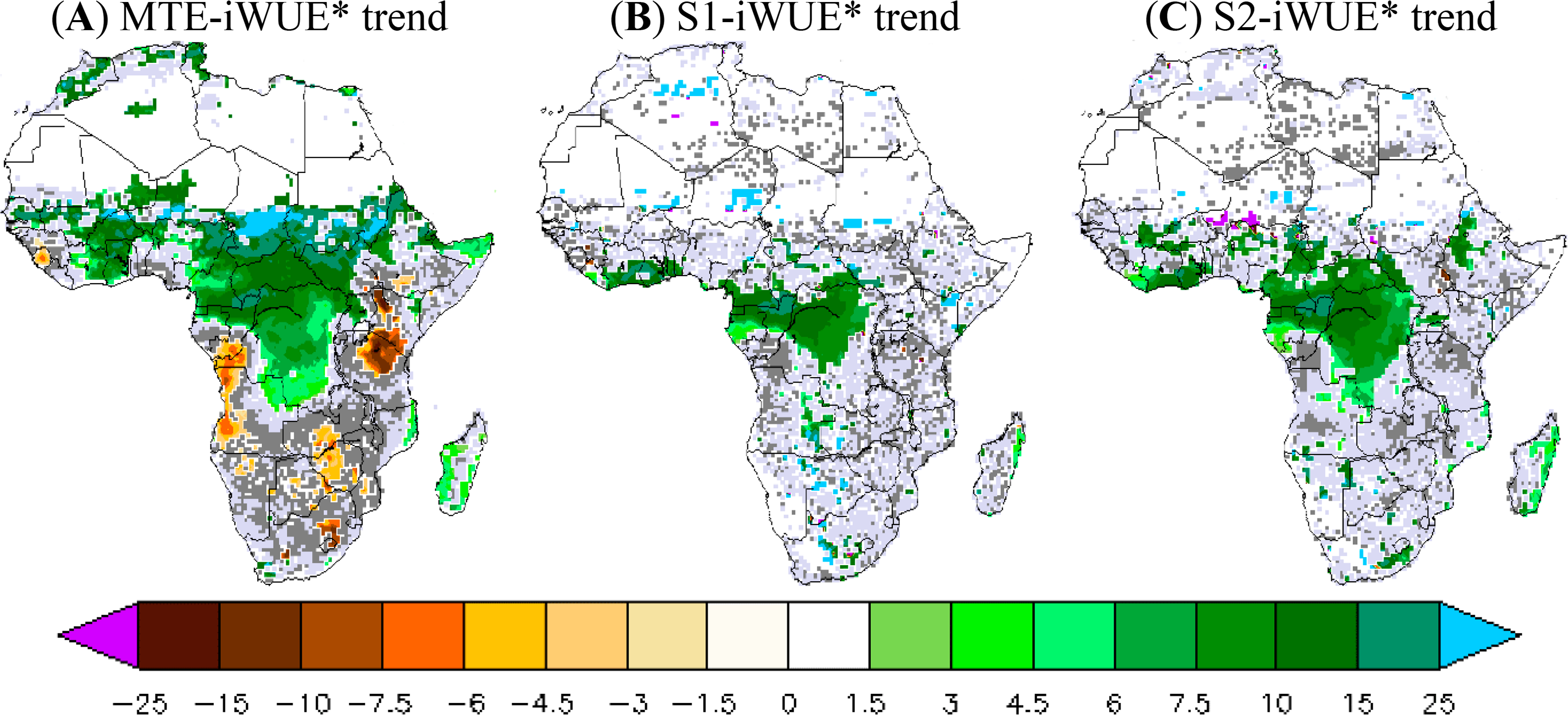
Figure 3 shows the results obtained with the validation datasets and the two ORCHIDEE simulations S1 and S2, in terms of temporal trends in annual iWUE* during 1982–2010. We found in the observational data a positive MTE-iWUE* trend during 1982–2010 (at 95% CI) over a large part of the African northern savannah and the African central forest. The iWUE* trend is between 5% and 20% of iWUE* per decade, which corresponds to a high and positive trend of the product GPP*VPD over the African northern savannahs and central forest (data not shown). In contrast, Kenya, Angola, and the southern part of Africa are marked with a negative and statistically significant trend of MTE-iWUE* (−5% to −10% per decade) corresponding to a negative trend of the product GPP*VPD. Compared to the MTE-iWUE* product, the simulated iWUE* trend at 95% CI is positive only over the central African forest. The geographical pattern of the 11-layer iWUE* trend at 95% CI is confined over the Central African forest and ranges from 7% to 20% of iWUE* per decade (Figure 3). The iWUE* trend from the 2-layer version is similar to that of the 11-layer version, but this version produces a statistically significant iWUE* trend covering more grid cells in the central African forest (Figure 3). The ORCHIDEE model, thus, does not reproduce the MTE-iWUE* trend over the northern savannahs. The model also does not reproduce the negative iWUE* trend in Kenyan, Angola, and the southern African areas (Figure 3).
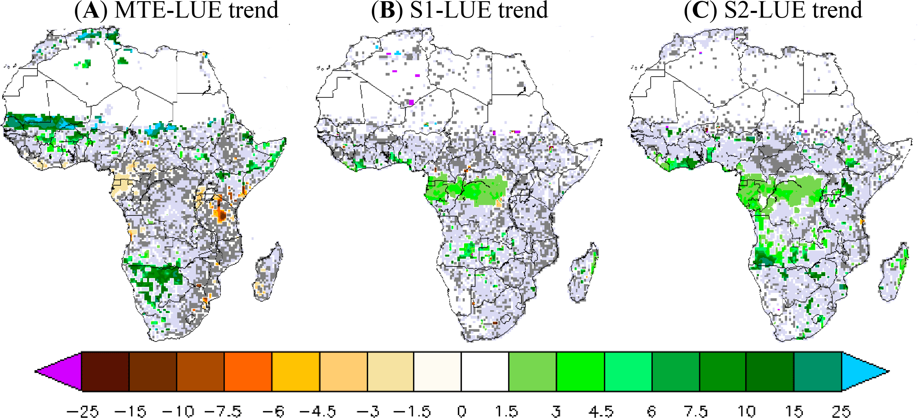
3.2.2. LUE Trend during 1982–2010
The LUE trend calculated by combining the MTE-GPP product and fAPAR3g is positive across the entire African continent but its significance is low, except for a few grid cells (Figure 4). The northwest of Sahel and Botswana show a positive MTE-LUE trend (15%–20% increase per decade) at 95% CI, whereas Cameroon (−2% per decade) and Tanzania (−7%) show negative MTE-LUE trends at 95% CI. In contrast to the MTE and fAPAR3g based product, the simulated LUE trend is positive only over the central African forest for both ORCHIDEE versions. The ORCHIDEE LUE trend varies between 2% and 5% per decade over central African forest. Note that the 2-layer version has a larger LUE trend at 95%CI of about 10% per decade in some grid cells over the southern of Angola (Figure 4). Overall, both versions of ORCHIDEE do not reproduce the observation-derived positive MTE-LUE trend in northwestern Sahel and the negative MTE-LUE trend over Cameroon and Kenyan zones (Figure 4).
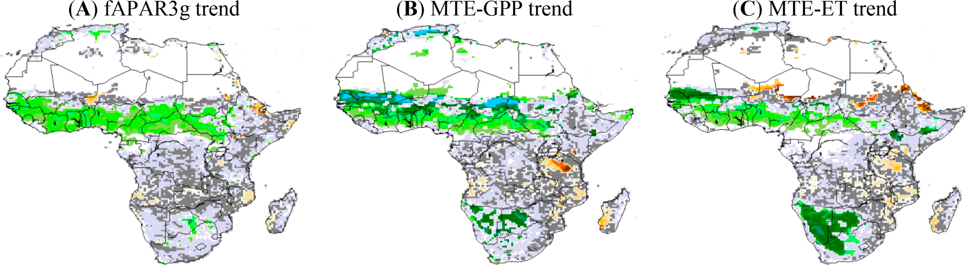
3.2.3. fAPAR3g, MTE-GPP and MTE-ETTrend during 1982–2010
To better understand the iWUE* and LUE trends, we analyzed the trends of fAPAR, GPP and ET separately. The comparison between the simulations and data-products for fAPAR, GPP and ET trends is shown in Figure 5. Both GIMMS satellite data and the MTE-GPP show positive trends (at 95% CI) over the northern savannahs, especially in West Africa for the MTE product. For example, fAPAR3g shows a robust and positive trend over the northern savannahs by 4% per decade (Figure 5A). However, the fAPAR3g trend calculated from the annual values does not show a significant trend during 1982–2010 over the Sahelian band, probably due to the compensation of trends between wet and dry seasons, especially for the last decade (fAPAR3g has a negative trend in dry season during 2000–2010 over the Sahel). The GPP from the MTE product shows a large positive trend at 95% CI over the northern savannah, particularly over the West African and Sahelian zone over which MTE-GPP increases by 25% per decade (Figure 5 B). A positive and strong MTE-ET trend at 95% CI is found over West Africa (more than 10% per decade over the Senegal) and the southern Sahel (4% per decade over the Guinea band). Over the African southern savannahs, ET increases significantly by 15% per decade during 1982–2010. Note however the negative trend in both MTE-ET and MTE-GPP over Tanzania with values of about −5% of decrease per decade.
Simulation results from both versions of ORCHIDEE (11-layer and 2-layer) show comparable geographical patterns of fAPAR, GPP and ET trends during 1982–2010. Contrary to the GIMMS-fAPAR3g trends, the ORCHIDEE model shows no significant temporal trend from annual fAPAR over a large part of Africa, regardless of the soil hydrology scheme. Areas of simulated fAPAR trend at 95% CI are patchy and include only few grid cells (Figure 5D,G). In comparison with MTE-GPP product, ORCHIDEE only simulates positive GPP trend at 95% CI over central African forest (4% per decade) for both soil hydrology schemes, and does not match the MTE-GPP product. However, ORCHIDEE simulates strong and positive GPP trend in some grid cells over the African southern savannahs (20% per decade) consistently with MTE-GPP (Figure 5E,H). As for GPP, the simulated ET trend does not match the geographical pattern of MTE-ET trend over the northern savannah. In contrast, the model better matches the MTE-ET trends over the African southern savannahs (Figure 5F,I). ORCHIDEE simulates a negative ET trend during 1982–2010 over the southern African forests (Zambia and Zimbabwe) of −4% per decade. Over the African southern savannahs, ORCHIDEE simulates a positive and strong ET trend during 1982–2010 in a few grid cells (15% of increase per decade).
3.3. CO2 and Climate Effect on iWUE* and LUE Trends
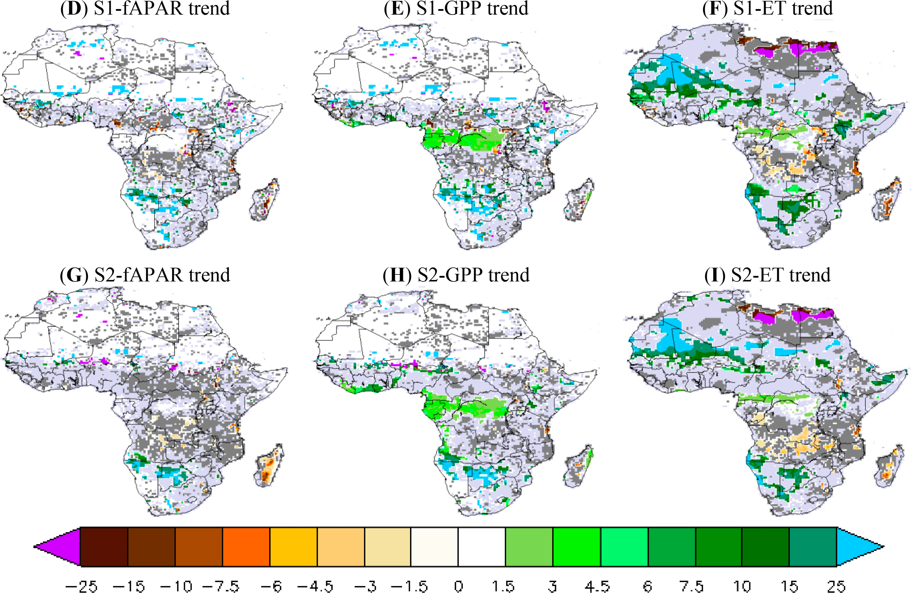
3.3.1. Atmospheric CO2 Effect on iWUE* and LUE Trends
The atmospheric CO2 effect on iWUE* and LUE trends is analyzed in Figure 6. We focus on the difference between the trends of S2 and S2-FIXCO2 simulations (Table 1). Hereafter, ΔiWUE* refers to the S2-iWUE* trend minus the S2-FIXCO2-iWUE* trend, and ΔLUE refers to the S2-LUE trend minus the S2-FIXCO2-LUE trend. We find a positive and high sensitivity of iWUE* and LUE trends to increasing atmospheric CO2, especially in the central African forest. ΔiWUE* is 30%–50% per decade (Figure 6A) of the S2-iWUE* trend, indicating that CO2 increase explains about half of the modeled iWUE* trend. The CO2 effects result found in this study, is consistent with previous studies in iWUE* [30,33,64]. Outside the central African forest, the CO2 effect on iWUE* trend is generally positive but the statistical significance is weak.
The LUE trend shows a very high sensitivity to atmospheric CO2 in comparison with the iWUE* trend. ΔLUE represents more than 100% of the S2-LUE trend over a large part of the central African forest, where a high and negative LUE trend is predicted if constant atmospheric CO2 is assumed. This high CO2 effect on LUE trend over the central African forest shows a high sensitivity of the ORCHIDEE model LUE to the atmospheric CO2 fertilization effect. Note also that the CO2 effect on the simulated LUE trends is globally positive over the whole continent but not statistically significant outside the central African forest (as seen with CO2 effect on the iWUE* trend).
3.3.2. A Source of Systematic Error: The Sensitivity of LUE and iWUE* Trends to Climate Forcing Data
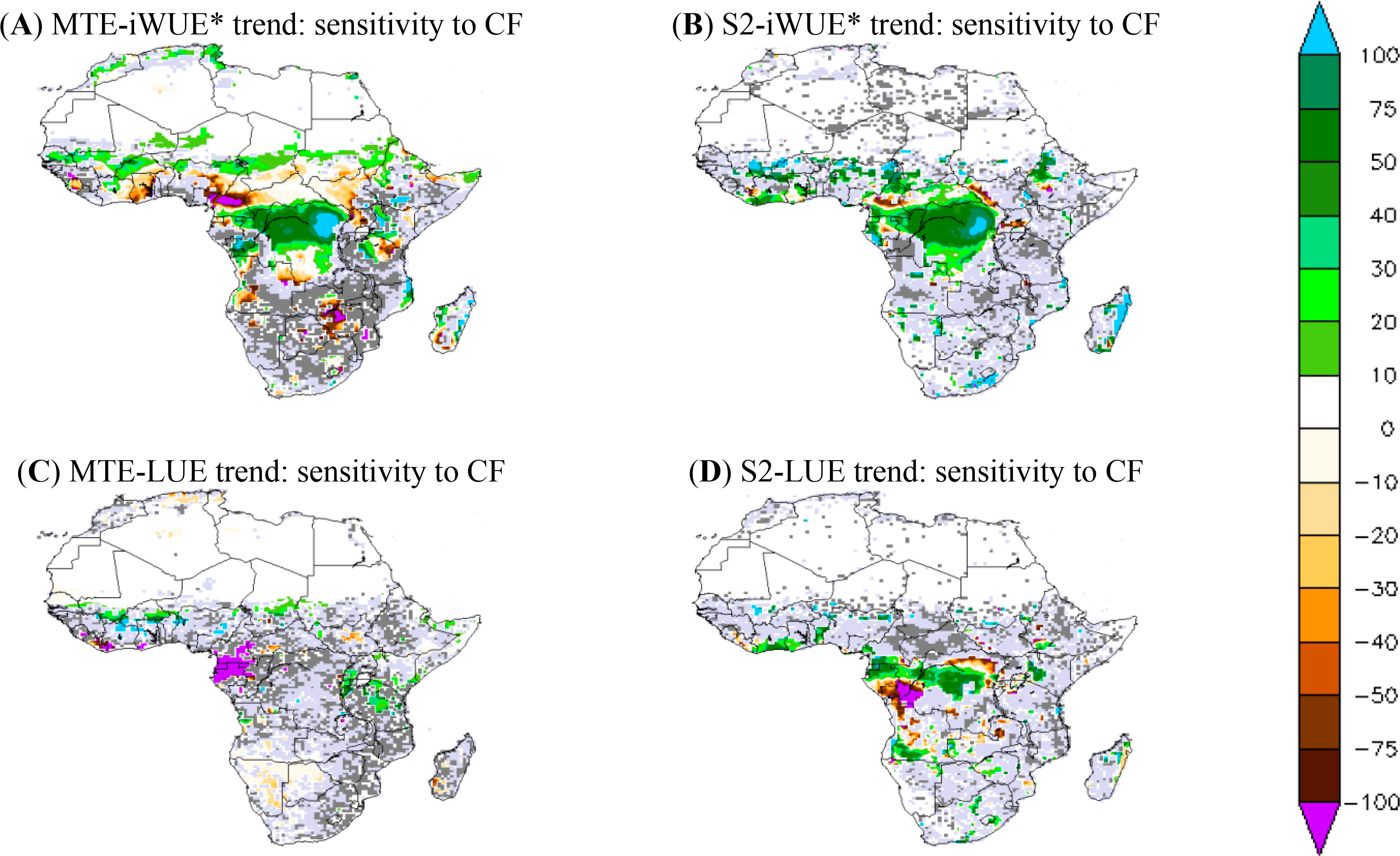
The sensitivity of simulated iWUE* and LUE trends to the choice of a climate forcing (CF) defined by the trend difference between S2 and S2-WFD simulations, which were obtained using WFDEI and WFD respectively, is shown in Figure 7. For the MTE product, the sensitivity of the iWUE* trend to CF is mainly related to differences in VPD trend between WFDEI and WFD (data not shown). The sensitivity of LUE trend to CF can be explained by differences of solar radiation trends between WFDEI and WFD.
The sensitivity of the iWUE* to CF is consistent between simulations and MTE-iWUE*, especially in the central African forest. The choice of CF, thus, has a significant effect on the iWUE* trend over the central African forest region. In fact the difference between iWUE* trends from the WFDEI and WFD CF reaches up to 75% of the iWUE* trend from WFDEI for both modeled and MTE products (Figure 7). In contrast, for the central African forest, the MTE-iWUE* trend obtained with WFDEI CF is weak over the northern savannahs, especially over Cameroon and South Sudan in comparison to that MTE-iWUE* calculated from the WFD CF. ORCHIDEE shows a weak sensitivity of iWUE* to CF over the Sahelian zone and Southern Africa, in contrast to the MTE product (Figure 7).
The sensitivity of the LUE trend to the choice of CF shows different geographical patterns between ORCHIDEE simulations and the calculated MTE-LUE (Figure 7). High sensitivity of the MTE-LUE trend to CF is sparse and mainly located over Cameroon and Gabon: the MTE-LUE trend obtained with WDF climate is negative and higher than the one obtained with WFDEI (Figure 7). In contrast to the MTE-LUE, the simulated LUE trend shows higher sensitivities to CF in the central African forest. The simulated LUE trend at 95% CI is positive with WFDEI-CF and larger than the one obtained with WFD climate over Cameroon, whereas LUE trend is weaker over Angola (Figure 7).
4. Discussions
The fAPAR3g used to calculate a LUE observation-based product was computed from the latest version of the GIMMS NDVI [40]. NDVI3g is calibrated using SeaWifs data during 1997–2010 [40], improving the data quality. The fAPAR3g trend during 1982–2010 computed from fAPAR annual values shows no significant trend over the Sahelian band. This result can be explained by the compensation between a positive fAPAR trend in growing seasons and a negative trend during the dry season [35,65–68].
The MTE algorithm is mainly trained on spatial gradients between flux towers to produce long-term series. However, no flux tower measurements were available to calibrate the MTE data-driven model over Africa, involving a moderate confidence in MTE products. The performance of MTE based on cross validation was found to be better for ET whereas MTE-GPP was found to be smaller than GPP deduced from GOSAT fluorescence data as a proxy or against MODIS GPP datasets [41,69–71]. This potential negative bias of MTE-GPP value could partly explain the low MTE-iWUE* values for Evergreen Broad-Leaved Forest ecosystems in comparison with, e.g., the flux tower data analyzed in [18].
The LUE trend that we constructed from observations can be analyzed as the difference between GPP trend and APAR trend. Over the northern savannahs, both GPP and APAR increased simultaneously during 1982–2010 and approximately in the same range. These GPP and APAR positive trends imply a stabilization of the LUE in the African northern savannahs during the last 30 years. Over the rest of Africa, there is no significant trend for both GPP and APAR.
Since the GPP and ET trends show a roughly comparable geographical pattern, especially over the southern Sahel (see Figure 5B,C), the geographical pattern of the iWUE* trend ends up being mainly explained by the VPD trend (data not shown). We found a strong positive VPD trend (from WFDEI) over the central African forest and the northern savannahs during 1982–2010 probably related to rising temperatures. This iWUE* increase, related to the positive VPD trend, reflects positive physiological responses of plant functional types to environmental changes, as found in previous studies in steppe or rainforest [28,72,73].
The LUE trend simulated by ORCHIDEE is only significant over the central African forest and matches the geographical pattern of the simulated GPP trend (Figure 4B,C compared to Figure 5E,H), since ORCHIDEE failed to simulate the significant fAPAR trend (calculated from annual value) over the northern savannahs as seen in fAPAR3g satellite data. The positive GPP trend simulated over the central Africa is probably due to the high sensitivity of ORCHIDEE to CO2 fertilization especially in forest areas.
The difficulties of ORCHIDEE to simulate a statistically significant ET trend over the northern savannahs could explain the low significance of the simulated iWUE* trend over these areas. As for LUE, ORCHIDEE only succeeds to produce a positive and significant iWUE* trend over the central African forest, which is highly related to the CO2 increase, and is consistent with the relationship between CO2 and iWUE* found in previous studies [30–33]. Note that the two versions of ORCHIDEE used in this study do not have as many differences in the spatial patterns of the trends compared to their averages, indicating that the soil diffusion scheme has no effect on fAPAR, GPP and ET trends but affects the mean values of these variables. Therefore, the difficulties of ORCHIDEE to reproduce geographical patterns of trends from satellite and data-driven model could be related to the phenology scheme instead of the soil hydrology model.
Besides the difference between the hydrological schemes of both ORCHIDEE versions, uncertainties from soil water availability on iWUE* and LUE trends are not specifically addressed in this study as well as ecological processes such as photosynthesis, respiration or fire. Soil moisture appears as a key factor for iWUE* and LUE trends and especially over steppe areas [60,73]. In addition, environmental factors such as cloudiness acts on iWUE* and LUE as well as vegetation photosynthesis and respiration [27,28,64]. It is, therefore, critical, for future studies, to analyze the environmental and ecological processes effects on the African iWUE* and LUE trends.
5. Conclusions
Previous studies have reported the sensitivity of light use efficiency (LUE) and inherent water use efficiency (iWUE*) to atmospheric CO2 increase, climate trends and land use change [27–34] with very few studies over Africa. These studies were mainly based on in situ measurements and focused on specific locations. The main novelty of this study is the use of recently available satellite data to investigate trends of LUE and iWUE* over African biomes for the past 30 years. The capability of a process based land surface model to reproduce the LUE and iWUE* trends in Africa was also analyzed, which can serve as a basis for evaluation of other models. In addition, we have attempted to attribute the effect of rising CO2 and the impact of two different gridded climate forcing datasets on LUE and iWUE* trends.
We found from satellite and climate observations that iWUE* increased significantly over the last three decades over the northern savannas and central African forest biomes (10%–20% per decade), consistent with the long-term increase in WUE observed at forest sites elsewhere [32,64,74–80]. The ORCHIDEE model only succeeded to reproduce a significant and positive iWUE* trend in the central African forest and not in savannas. Between 30% and 50% of the simulated iWUE* trend is attributed to the increased atmospheric CO2. We note however that diagnosing trends of iWUE* is subject to systematic errors related to the use of a specific climate forcing dataset. This source of error is very important over the central African forest. This result shows the importance of having accurate climatic historical reconstructions to investigate iWUE* and LUE trends in observations and in models as recently pointed out for drought trends as well [81,82].
In opposite to iWUE* trend, the observation-derived LUE trend is not statistically significant over most part of Africa. In contrast to the observations, ORCHIDEE shows a 5% LUE increase per decade in central African forest, probably due to the high CO2 fertilization effect of the model, particularly in forest ecosystems. The simulated LUE trend shows an opposite sign depending on whether rising CO2 is included or not in the simulation. The effect on simulated LUE trend caused the use of a specific climate forcing is important, especially over Cameroon, for the observation-based product, whereas ORCHIDEE shows a sensitivity to climate forcing over the central African forest.
The way forward to improve ORCHIDEE simulations of LUE and iWUE* is a better representation of phenology using e.g.,in situ observations for calibration. Because the trends of annual LUE and iWUE* can result from different responses during different seasons, evaluation of LUE and iWUE* seasonal trends and variability is a priority for future studies. Finally, it will be necessary to analyze land use change effects on LUE and iWUE* in regions where agricultural area and practice have changed significantly over the last decade.
Acknowledgments
This work is supported by the ClimAfrica project funded by the European Commission under the 7th Framework Programme (FP7). We are grateful to the GIMMS group for sharing the NDVI3g data (we thank Zaichun Zhu and Ranga B. Myneni). Through Martin Jung, we are thankful to the Department Biogeochemical Integration at the Max Planck Institute for Biogeochemistry for providing Monthly gross primary productivity and evapotranspiration deduced from FLUXNET data from the “La-Thuile-2007” synthesis effort.
Author Contributions
All authors contributed extensively to the work presented in this paper. R. Myneni and M. Jung provided respectively fAPAR3g data and MTE-GPP/ET products. A. Traore, Philippe Ciais and Nicolas Vuichard designed the experiments and carrier out the interpretation of the results. A. Traore and Philippe Ciais drafted the manuscript, which was revised by all authors. All authors read and approved the final manuscript.
Conflicts of Interest
The authors declare no conflict of interest.
References
- Mercado, L.M.; Bellouin, N.; Sitch, S.; Boucher, O.; Huntingford, C.; Wild, M.; Cox, P.M. Impact of changes in diffuse radiation on the global land carbon sink. Nature 2009, 458, 1014–1017. [Google Scholar]
- Baldocchi, D. TURNER REVIEW No. 15. “Breathing” of the terrestrial biosphere: Lessons learned from a global network of carbon dioxide flux measurement systems”. Aust. J. Bot 2008, 56, 1–26. [Google Scholar]
- Rocha, A.V.; Hong-Bing, S.; Vogel, C.S.; Peter, S.H.; Curtis, P.S. Photosynthetic and water use efficiency responses to diffuse radiation by an aspen-dominated northern hardwood forest. For. Sci 2004, 50, 793–801. [Google Scholar]
- Urban, O.; Janus, D.; Acosta, M.; Czerny, R.; Markova, I.; NavrATil, M.; Pavelka, M.; Pokorny, R.; Šprtova, M.; Zhang, R. Ecophysiological controls over the net ecosystem exchange of mountain spruce stand. Comparison of the response in direct vs. diffuse solar radiation. Glob. Chang. Biol 2007, 13, 157–168. [Google Scholar]
- Seneviratne, S.I.; Corti, T.; Davin, E.L.; Hirschi, M.; Jaeger, E.B.; Lehner, I.; Orlowsky, B.; Teuling, A.J. Investigating soil moisture–climate interactions in a changing climate: A review. Earth-Sci. Rev 2010, 99, 125–161. [Google Scholar]
- Jung, M.; Reichstein, M.; Ciais, P.; Seneviratne, S.I.; Sheffield, J.; Goulden, M.L.; Bonan, G.; Cescatti, A.; Chen, J.; de Jeu, R. Recent decline in the global land evapotranspiration trend due to limited moisture supply. Nature 2010, 467, 951–954. [Google Scholar]
- Budyko, M. Climate and Life, 508; Academic: San Diego, CA, USA, 1974. [Google Scholar]
- Menaut, J.; Barbault, R.; Lavelle, P.; Lepage, M. African Savannas: Biological Systems of Humification and Mineralization. In Ecology and Management of the World’s Savannas; Tothill, J.C., Mott, J.J., Eds.; Australian Academy of Science: Canberra, Australian, 1984; pp. 14–33. [Google Scholar]
- Huxman, T.E.; Snyder, K.A.; Tissue, D.; Leffler, A.J.; Ogle, K.; Pockman, W.T.; Sandquist, D.R.; Potts, D.L.; Schwinning, S. Precipitation pulses and carbon fluxes in semiarid and arid ecosystems. Oecologia 2004, 141, 254–268. [Google Scholar]
- Schwinning, S.; Sala, O.E. Hierarchy of responses to resource pulses in arid and semi-arid ecosystems. Oecologia 2004, 141, 211–220. [Google Scholar]
- Schwinning, S.; Sala, O.E.; Loik, M.E.; Ehleringer, J.R. Thresholds, memory, and seasonality: Understanding pulse dynamics in arid/semi-arid ecosystems. Oecologia 2004, 141, 191–193. [Google Scholar]
- Potts, D.; Huxman, T.; Cable, J.; English, N.; Ignace, D.; Eilts, J.; Mason, M.; Weltzin, J.; Williams, D. Antecedent moisture and seasonal precipitation influence the response of canopy-scale carbon and water exchange to rainfall pulses in a semi-arid grassland. New Phytol 2006, 170, 849–860. [Google Scholar]
- Webb, W.L.; Lauenroth, W.K.; Szarek, S.R.; Kinerson, R.S. Primary production and abiotic controls in forests, grasslands, and desert ecosystems in the United States. Ecology 1983, 64, 134–151. [Google Scholar]
- Running, S.W.; Nemani, R.R.; Heinsch, F.A.; Zhao, M.; Reeves, M.; Hashimoto, H. A continuous satellite-derived measure of global terrestrial primary production. Bioscience 2004, 54, 547–560. [Google Scholar]
- Landsberg, J.J.; Sands, P. Physiological Ecology of Forest Production: Principles, Processes and Models; Academic Press: London, UK, 2010; Volume 4. [Google Scholar]
- Gu, L.; Baldocchi, D.; Verma, S.B.; Black, T.; Vesala, T.; Falge, E.M.; Dowty, P.R. Advantages of diffuse radiation for terrestrial ecosystem productivity. J. Geophys. Res. Atmos. (1984–2012) 2002, 107. [Google Scholar] [CrossRef]
- Alton, P.; North, P.; Los, S. The impact of diffuse sunlight on canopy light-use efficiency, gross photosynthetic product and net ecosystem exchange in three forest biomes. Glob. Chang. Biol 2007, 13, 776–787. [Google Scholar]
- Beer, C.; Ciais, P.; Reichstein, M.; Baldocchi, D.; Law, B.; Papale, D.; Soussana, J.F.; Ammann, C.; Buchmann, N.; Frank, D. Temporal and among-site variability of inherent water use efficiency at the ecosystem level. Glob. Biogeochem. Cycles 2009, 23. [Google Scholar] [CrossRef]
- Lange, O.L.; Lösch, R.; Schulze, E.-D.; Kappen, L. Responses of stomata to changes in humidity. Planta 1971, 100, 76–86. [Google Scholar]
- Schulze, E.-D.; Hall, A. Stomatal responses, water loss and CO2 assimilation rates of plants in contrasting environments. In Physiological Plant Ecology II; Springer: Berlin, Germany, 1982; pp. 181–230. [Google Scholar]
- Giannini, A.; Saravanan, R.; Chang, P. Oceanic forcing of sahel rainfall on interannual to interdecadal time scales. Science 2003, 302, 1027–1030. [Google Scholar]
- Nicholson, S.E. The West African Sahel: A review of recent studies on the rainfall regime and its interannual variability. ISRN Meteorol 2013, 2013. [Google Scholar] [CrossRef]
- Page, Y.L.; Pereira, J.; Trigo, R.; Camara, C.D.; Oom, D.; Mota, B. Global fire activity patterns (1996–2006) and climatic influence: An analysis using the World Fire Atlas. Atmos. Chem. Phys 2008, 8, 1911–1924. [Google Scholar]
- Anyamba, A.; Justice, C.; Tucker, C.; Mahoney, R. Seasonal to interannual variability of vegetation and fires at SAFARI 2000 sites inferred from advanced very high resolution radiometer time series data. J. Geophys. Res. Atmos. (1984–2012) 2003, 108. [Google Scholar] [CrossRef]
- Anyamba, A.; Tucker, C.J.; Mahoney, R. From El Niño to La Niña: Vegetation response patterns over East and Southern Africa during the 1997–2000 period. J.Clim 2002, 15, 3096–3103. [Google Scholar]
- Ciais, P.; Piao, S.-L.; Cadule, P.; Friedlingstein, P.; Chédin, A. Variability and recent trends in the African terrestrial carbon balance. Biogeosciences 2009, 6, 1935–1948. [Google Scholar]
- Zhang, M.; Yu, G.-R.; Zhuang, J.; Gentry, R.; Fu, Y.-L.; Sun, X.-M.; Zhang, L.-M.; Wen, X.-F.; Wang, Q.-F.; Han, S.-J. Effects of cloudiness change on net ecosystem exchange, light use efficiency, and water use efficiency in typical ecosystems of China. Agric. For. Meteorol 2011, 151, 803–816. [Google Scholar]
- Tong, X.; Zhang, J.; Meng, P.; Li, J.; Zheng, N. Ecosystem water use efficiency in a warm-temperate mixed plantation in the North China. J. Hydrol 2014, 512, 221–228. [Google Scholar]
- Nakaji, T.; Kosugi, Y.; Takanashi, S.; Niiyama, K.; Noguchi, S.; Tani, M.; Oguma, H.; Nik, A.R.; Kassim, A.R. Estimation of light-use efficiency through a combinational use of the photochemical reflectance index and vapor pressure deficit in an evergreen tropical rainforest at Pasoh, Peninsular Malaysia. Remote Sens. Environ 2014, 150, 82–92. [Google Scholar]
- Keenan, T.F.; Hollinger, D.Y.; Bohrer, G.; Dragoni, D.; Munger, J.W.; Schmid, H.P.; Richardson, A.D. Increase in forest water-use efficiency as atmospheric carbon dioxide concentrations rise. Nature 2013, 499, 324–327. [Google Scholar]
- Körner, C. Responses of humid tropical trees to rising CO2. Annu. Rev. Ecol. Evol. Syst 2009, 40, 61–79. [Google Scholar]
- Feng, X. Trends in intrinsic water-use efficiency of natural trees for the past 100–200 years: A response to atmospheric CO2 concentration. Geochim. Cosmochim. Acta 1999, 63, 1891–1903. [Google Scholar]
- Kauwe, M.G.; Medlyn, B.E.; Zaehle, S.; Walker, A.P.; Dietze, M.C.; Hickler, T.; Jain, A.K.; Luo, Y.; Parton, W.J.; Prentice, I.C. Forest water use and water use efficiency at elevated CO2: A model-data intercomparison at two contrasting temperate forest FACE sites. Glob.Chang.Biol 2013, 19, 1759–1779. [Google Scholar]
- Medlyn, B.; de Kauwe, M. Biogeochemistry: Carbon dioxide and water use in forests. Nature 2013, 499, 287–289. [Google Scholar]
- Dardel, C.; Kergoat, L.; Hiernaux, P.; Mougin, E.; Grippa, M.; Tucker, C. Re-Greening Sahel: 30 years of remote sensing data and field observations (Mali, Niger). Remote Sens. Environ 2014, 140, 350–364. [Google Scholar]
- Ciais, P.; Bombelli, A.; Williams, M.; Piao, S.L.; Chave, J.; Ryan, C.M.; Henry, M.; Brender, P.; Valentini, R. The carbon balance of Africa: Synthesis of recent research studies. Philos. Trans. R. Soc. A: Math. Phys. Eng. Sci 2011, 369, 2038–2057. [Google Scholar]
- Jung, M.; Reichstein, M.; Bondeau, A. Towards global empirical upscaling of FLUXNET eddy covariance observations: Validation of a model tree ensemble approach using a biosphere model. Biogeosciences 2009, 6. [Google Scholar] [CrossRef]
- Yuan, X.; Wood, E.F.; Luo, L.; Pan, M. A first look at Climate Forecast System version 2 (CFSv2) for hydrological seasonal prediction. Geophys. Res. Lett 2011, 38. [Google Scholar] [CrossRef]
- Weber, U.; Jung, M.; Reichstein, M.; Beer, C.; Braakhekke, M.; Lehsten, V.; Ghent, D.; Kaduk, J.; Viovy, N.; Ciais, P. The inter-annual variability of Africa’s ecosystem productivity: A multi-model analysis. Biogeosci. Discuss 2008, 5, 4035–4069. [Google Scholar]
- Zhu, Z.; Bi, J.; Pan, Y.; Ganguly, S.; Anav, A.; Xu, L.; Samanta, A.; Piao, S.; Nemani, R.R.; Myneni, R.B. Global data sets of vegetation leaf area index (LAI) 3g and Fraction of Photosynthetically Active Radiation (FPAR) 3g derived from Global Inventory Modeling and Mapping Studies (GIMMS) Normalized Difference Vegetation Index (NDVI3g) for the period 1981 to 2011. Remote Sens 2013, 5, 927–948. [Google Scholar]
- Jung, M.; Reichstein, M.; Margolis, H.A.; Cescatti, A.; Richardson, A.D.; Arain, M.A.; Arneth, A.; Bernhofer, C.; Bonal, D.; Chen, J. Global patterns of land-atmosphere fluxes of carbon dioxide, latent heat, and sensible heat derived from eddy covariance, satellite, and meteorological observations. J. Geophys. Res. Biogeosci. (2005–2012) 2011, 116. [Google Scholar] [CrossRef]
- Krinner, G.; Viovy, N.; de Noblet-Ducoudré, N.; Ogée, J.; Polcher, J.; Friedlingstein, P.; Ciais, P.; Sitch, S.; Prentice, I.C. A dynamic global vegetation model for studies of the coupled atmosphere-biosphere system. Glob. Biogeochem. Cycles 2005, 19. [Google Scholar] [CrossRef]
- Farquhar, G.; von Caemmerer, S.V.; Berry, J. A biochemical model of photosynthetic CO2 assimilation in leaves of C3 species. Planta 1980, 149, 78–90. [Google Scholar]
- Collatz, G.J.; Ribas-Carbo, M.; Berry, J. Coupled photosynthesis-stomatal conductance model for leaves of C4 plants. Funct. Plant Biol 1992, 19, 519–538. [Google Scholar]
- Ruimy, A.; Kergoat, L.; Bondeau, A. Comparing global models of terrestrial net primary productivity (NPP): Analysis of differences in light absorption and light-use efficiency. Glob. Chang. Biol 1999, 5, 56–64. [Google Scholar]
- Ducoudré, N.I.; Laval, K.; Perrier, A. SECHIBA, a new set of parameterizations of the hydrologic exchanges at the land-atmosphere interface within the LMD atmospheric general circulation model. J. Clim 1993, 6, 248–273. [Google Scholar]
- De Rosnay, P.; Polcher, J. Modelling root water uptake in a complex land surface scheme coupled to a GCM. Hydrol. Earth Syst. Sci 1998, 2, 239–255. [Google Scholar]
- McMurtrie, R.; Rook, D.; Kelliher, F. Modelling the yield ofPinus radiata on a site limited by water and nitrogen. For. Ecol. Manag 1990, 30, 381–413. [Google Scholar]
- De Rosnay, P.; Polcher, J.; Laval, K.; Sabre, M. Integrated parameterization of irrigation in the land surface model ORCHIDEE. Validation over Indian Peninsula. Geophys. Res. Lett 2003, 30. [Google Scholar] [CrossRef]
- D’Orgeval, T. Impact du Changement Climatique sur le cycle de l’eau en Afrique de l’Ouest: modéLisation et Incertitudes. Available online: http://dods.ipsl.jussieu.fr/orchidee/WEBORCHIDEE/ANOTER/These_dOrgeval.pdf (accessed on 19 September 2014).
- Campoy, A.; Ducharne, A.; Cheruy, F.; Hourdin, F.; Polcher, J.; Dupont, J. Influence of soil bottom hydrological conditions on land surface fluxes and climate in a general circulation model. Geophys. Res.-Atmos 2013, 118, 10725–10739. [Google Scholar]
- Richards, L.A. Capillary conduction of liquids through porous mediums. J. Appl. Phys 2004, 1, 318–333. [Google Scholar]
- Bruen, M. Sensitivity of Hydrological Processes at the Land-Atmosphere Interface, in Global Change and the Irish Environment; Sweeney, J., Ed.; Sweeney Royal Irish Academy: Dublin, Ireland, 1997. [Google Scholar]
- Dooge, J.C.; Dowley, A. Final Report on EU Funded (PL890016 EPOCH) Project on Spatial Variability of Land Surface Processes (SLAPS); University College: Dublin, Irish, 1993; p. 144. [Google Scholar]
- Weedon, G.; Gomes, S.; Viterbo, P.; Shuttleworth, W.; Blyth, E.; Österle, H.; Adam, J.; Bellouin, N.; Boucher, O.; Best, M. Creation of the WATCH forcing data and its use to assess global and regional reference crop evaporation over land during the twentieth century. J. Hydrometeorol 2011, 12, 823–848. [Google Scholar]
- Dee, D.; Uppala, S.; Simmons, A.; Berrisford, P.; Poli, P.; Kobayashi, S.; Andrae, U.; Balmaseda, M.; Balsamo, G.; Bauer, P. The ERA-Interim reanalysis: Configuration and performance of the data assimilation system. Quart. J. R. Meteorol. Soc 2011, 137, 553–597. [Google Scholar]
- Schneider, U.; Becker, A.; Finger, P.; Meyer-Christoffer, A.; Ziese, M.; Rudolf, B. GPCC’s new land surface precipitation climatology based on quality-controlled in situ data and its role in quantifying the global water cycle. Theor. Appl. Climatol 2014, 115, 15–40. [Google Scholar]
- Weedon, G.; Gomes, S.; Viterbo, P.; Österle, H.; Adam, J.; Bellouin, N.; Boucher, O.; Best, M. The WATCH Forcing Data 1958–2001: A Meteorological Forcing Dataset for Land Surface and Hydrological Models; WATCH Technical Report;Met Office, Hadley Centre: Exeter, UK, 2010. [Google Scholar]
- Lardy, R.; Bellocchi, G.; Soussana, J.-F. A new method to determine soil organic carbon equilibrium. Environ. Modell. Softw 2011, 26, 1759–1763. [Google Scholar]
- Yuan, W.; Liu, S.; Zhou, G.; Zhou, G.; Tieszen, L.L.; Baldocchi, D.; Bernhofer, C.; Gholz, H.; Goldstein, A.H.; Goulden, M.L. Deriving a light use efficiency model from eddy covariance flux data for predicting daily gross primary production across biomes. Agric. For. Meteorol 2007, 143, 189–207. [Google Scholar]
- Jacovides, C.; Tymvios, F.; Asimakopoulos, D.; Theofilou, K.; Pashiardes, S. Global photosynthetically active radiation and its relationship with global solar radiation in the Eastern Mediterranean basin. Theor. Appl. Climatol 2003, 74, 227–233. [Google Scholar]
- Tsubo, M.; Walker, S. Relationships between photosynthetically active radiation and clearness index at Bloemfontein, South Africa. Theor. Appl. Climatol 2005, 80, 17–25. [Google Scholar]
- Goldewijk, K.K.; Beusen, A.; van Drecht, G.; de Vos, M. The HYDE 3.1 spatially explicit database of human-induced global land-use change over the past 12,000 years. Glob. Ecol. Biogeogr 2011, 20, 73–86. [Google Scholar]
- Nock, C.A.; Baker, P.J.; Wanek, W.; Leis, A.; Grabner, M.; Bunyavejchewin, S.; Hietz, P. Long-term increases in intrinsic water-use efficiency do not lead to increased stem growth in a tropical monsoon forest in western Thailand. Glob. Chang. Biol 2011, 17, 1049–1063. [Google Scholar]
- Eklundh, L.; Olsson, L. Vegetation index trends for the African Sahel 1982–1999. Geophys. Res.Lett 2003, 30. [Google Scholar] [CrossRef]
- Olsson, L.; Eklundh, L.; Ardö, J. A recent greening of the Sahel—Trends, patterns and potential causes. J. Arid Environ 2005, 63, 556–566. [Google Scholar]
- Fensholt, R.; Langanke, T.; Rasmussen, K.; Reenberg, A.; Prince, S.D.; Tucker, C.; Scholes, R.J.; Le, Q.B.; Bondeau, A.; Eastman, R. Greenness in semi-arid areas across the globe 1981–2007—An earth observing satellite based analysis of trends and drivers. Remote Sens. Environ 2012, 121, 144–158. [Google Scholar]
- De Jong, R.; de Bruin, S.; de Wit, A.; Schaepman, M.E.; Dent, D.L. Analysis of monotonic greening and browning trends from global NDVI time-series. Remote Sens. Environ 2011, 115, 692–702. [Google Scholar]
- Frankenberg, C.; Fisher, J.B.; Worden, J.; Badgley, G.; Saatchi, S.S.; Lee, J.E.; Toon, G.C.; Butz, A.; Jung, M.; Kuze, A. New global observations of the terrestrial carbon cycle from GOSAT: Patterns of plant fluorescence with gross primary productivity. Geophys. Res.Lett 2011, 38. [Google Scholar] [CrossRef]
- Frankenberg, C.; O’Dell, C.; Guanter, L.; McDuffie, J. Remote sensing of near-infrared chlorophyll fluorescence from space in scattering atmospheres: Implications for its retrieval and interferences with atmospheric CO2 retrievals. Atmos. Meas. Techn 2012, 5, 2081–2094. [Google Scholar]
- Zhao, M.; Heinsch, F.A.; Nemani, R.R.; Running, S.W. Improvements of the MODIS terrestrial gross and net primary production global data set. Remote Sens. Environ 2005, 95, 164–176. [Google Scholar]
- Loader, N.J.; Walsh, R.P.D.; Robertson, I.; Bidin, K.; Ong, R.C.; Reynolds, G.; McCarroll, D.; Gagen, M.; Young, G. Recent trends in the intrinsic water-use efficiency of ringless rainforest trees in Borneo. Philos. Trans. R. Soc. B: Biol. Sci 2011, 366, 3330–3339. [Google Scholar]
- Li, S.G.; Eugster, W.; Asanuma, J.; Kotani, A.; Davaa, G.; Oyunbaatar, D.; Sugita, M. Response of gross ecosystem productivity, light use efficiency, and water use efficiency of Mongolian steppe to seasonal variations in soil moisture. J. Geophys. Res. Biogeosci. (2005–) 2008, 113. [Google Scholar] [CrossRef]
- Silva, L.C.; Anand, M.; Oliveira, J.M.; Pillar, V.D. Past century changes in Araucaria angustifolia (Bertol.) Kuntze water use efficiency and growth in forest and grassland ecosystems of southern Brazil: Implications for forest expansion. Glob. Chang. Biol 2009, 15, 2387–2396. [Google Scholar]
- Penuelas, J.; Hunt, J.M.; Ogaya, R.; Jump, A.S. Twentieth century changes of tree-ring δ13C at the southern range-edge of Fagus sylvatica: Increasing water-use efficiency does not avoid the growth decline induced by warming at low altitudes. Glob. Chang. Biol 2008, 14, 1076–1088. [Google Scholar]
- Hietz, P.; Wanek, W.; Dünisch, O. Long-term trends in cellulose δ13 C and water-use efficiency of tropical Cedrela and Swietenia from Brazil. Tree Physiol 2005, 25, 745–752. [Google Scholar]
- Saurer, M.; Siegwolf, R.T.; Schweingruber, F.H. Carbon isotope discrimination indicates improving water-use efficiency of trees in northern Eurasia over the last 100 years. Glob. Chang. Biol 2004, 10, 2109–2120. [Google Scholar]
- Duquesnay, A.; Breda, N.; Stievenard, M.; Dupouey, J. Changes of tree-ring δ13C and water-use efficiency of beech (Fagus sylvatica L.) in north-eastern France during the past century. Plant Cell Environ 1998, 21, 565–572. [Google Scholar]
- Bert, D.; Leavitt, S.W.; Dupouey, J.-L. Variations of wood δ13C and water-use efficiency of Abies alba during the last century. Ecology 1997, 78, 1588–1596. [Google Scholar]
- Linares, J.-C.; Delgado-Huertas, A.; Camarero, J.J.; Merino, J.; Carreira, J.A. Competition and drought limit the response of water-use efficiency to rising atmospheric carbon dioxide in the Mediterranean fir Abies pinsapo. Oecologia 2009, 161, 611–624. [Google Scholar]
- Trenberth, K.E.; Dai, A.; van der Schrier, G.; Jones, P.D.; Barichivich, J.; Briffa, K.R.; Sheffield, J. Global warming and changes in drought. Nat. Clim. Chang 2014, 4, 17–22. [Google Scholar]
- Sheffield, J.; Wood, E.F.; Roderick, M.L. Little change in global drought over the past 60 years. Nature 2012, 491, 435–438. [Google Scholar]


| Experiment | Model Version | Transient CO2 | Climate Forcing |
|---|---|---|---|
| S1 | 11-layer | Yes | WFDEI |
| S2 | 2-layer | Yes | WFDEI |
| S2-FIXCO2 | 2-layer | 336.5 ppm | WFDEI |
| S2-WFD | 2-layer | Yes | WFD |
© 2014 by the authors; licensee MDPI, Basel, Switzerland This article is an open access article distributed under the terms and conditions of the Creative Commons Attribution license (http://creativecommons.org/licenses/by/3.0/).
Share and Cite
Traore, A.K.; Ciais, P.; Vuichard, N.; MacBean, N.; Dardel, C.; Poulter, B.; Piao, S.; Fisher, J.B.; Viovy, N.; Jung, M.; et al. 1982–2010 Trends of Light Use Efficiency and Inherent Water Use Efficiency in African vegetation: Sensitivity to Climate and Atmospheric CO2 Concentrations. Remote Sens. 2014, 6, 8923-8944. https://0-doi-org.brum.beds.ac.uk/10.3390/rs6098923
Traore AK, Ciais P, Vuichard N, MacBean N, Dardel C, Poulter B, Piao S, Fisher JB, Viovy N, Jung M, et al. 1982–2010 Trends of Light Use Efficiency and Inherent Water Use Efficiency in African vegetation: Sensitivity to Climate and Atmospheric CO2 Concentrations. Remote Sensing. 2014; 6(9):8923-8944. https://0-doi-org.brum.beds.ac.uk/10.3390/rs6098923
Chicago/Turabian StyleTraore, Abdoul Khadre, Philippe Ciais, Nicolas Vuichard, Natasha MacBean, Cecile Dardel, Benjamin Poulter, Shilong Piao, Joshua B. Fisher, Nicolas Viovy, Martin Jung, and et al. 2014. "1982–2010 Trends of Light Use Efficiency and Inherent Water Use Efficiency in African vegetation: Sensitivity to Climate and Atmospheric CO2 Concentrations" Remote Sensing 6, no. 9: 8923-8944. https://0-doi-org.brum.beds.ac.uk/10.3390/rs6098923