UAV Remote Sensing for Urban Vegetation Mapping Using Random Forest and Texture Analysis

Abstract

Unmanned aerial vehicle (UAV) remote sensing has great potential for vegetation mapping in complex urban landscapes due to the ultra-high resolution imagery acquired at low altitudes. Because of payload capacity restrictions, off-the-shelf digital cameras are widely used on medium and small sized UAVs. The limitation of low spectral resolution in digital cameras for vegetation mapping can be reduced by incorporating texture features and robust classifiers. Random Forest has been widely used in satellite remote sensing applications, but its usage in UAV image classification has not been well documented. The objectives of this paper were to propose a hybrid method using Random Forest and texture analysis to accurately differentiate land covers of urban vegetated areas, and analyze how classification accuracy changes with texture window size. Six least correlated second-order texture measures were calculated at nine different window sizes and added to original Red-Green-Blue (RGB) images as ancillary data. A Random Forest classifier consisting of 200 decision trees was used for classification in the spectral-textural feature space. Results indicated the following: (1) Random Forest outperformed traditional Maximum Likelihood classifier and showed similar performance to object-based image analysis in urban vegetation classification; (2) the inclusion of texture features improved classification accuracy significantly; (3) classification accuracy followed an inverted U relationship with texture window size. The results demonstrate that UAV provides an efficient and ideal platform for urban vegetation mapping. The hybrid method proposed in this paper shows good performance in differentiating urban vegetation mapping. The drawbacks of off-the-shelf digital cameras can be reduced by adopting Random Forest and texture analysis at the same time.

1. Introduction

1.1. Urban Vegetation Mapping

Vegetation plays an important role in urban environments from many prospects, i.e., alleviating urban heat island effect, maintaining ecological balance, protecting biodiversity and promoting quality of life [1,2,3,4,5,6,7,8,9,10,11]. Urban vegetation mapping can be defined as the identification of land cover types over urban vegetated areas according to many studies [11]. It is highly necessary to produce these detailed vegetation maps to assist planners in designing strategies for the optimization of urban ecosystem services and climate change adaptation [11].

With the capacity for discriminating large scale of land cover types, remote sensing has been widely used for vegetation mapping in different environments [1,2,3]. Satellite imagery and aerial photography have been adopted for monitoring vegetation both in urban and wild areas [4,5,6,7]. Compared with wild vegetation (e.g., rangeland, forests), urban vegetation cover is much more divided and fragmented which is more difficult and challenging for accurate extraction. How to accurately map and extract land cover types over urban vegetated areas has been a hot topic in remote sensing field [1,2,3,4,5,6,7,8,9,10].

Generally, data used in urban vegetation mapping varies from moderate to high resolution (HR) and very high resolution (VHR) satellite imagery, VHR piloted aerial photography and ultra-high resolution (UHR) unmanned aerial vehicle images. For the moderate resolution multispectral satellite imagery (e.g., Landsat Thematic Mapper (TM), Enhanced Thematic Mapper Plus (ETM+)), the main drawback is that they lack the capability to capture enough details of ground objects due to coarse ground resolution (30 m). Nevertheless, they can still be used to quantify vegetation abundance in urban and suburban areas through spectral mixture analysis. A fraction map can be made to monitor the spatio-temporal variation of urban vegetation [2,6,10].

With the rapid development of remote sensing technology, HR and VHR satellite data like IKONOS and QuickBird have been successfully used for urban vegetation mapping due to their finer spatial resolution [3,4,8]. Aerial photography is also widely used because the images acquired have an even higher resolution [7]. Pixel-based image classification and object-based image analysis (OBIA) are widely used in classifying HR remote sensing images [1,2,3,4,5,6,7,8,9,10,11,12,13,14,15]. The former assumes that individual pixels are independent and they are treated without considering any spatial association with neighboring pixels [16]. However, single pixels no longer capture the characteristics of classification targets in HR images [17], and a “salt and pepper” effect is always obviously shown in the classification results. Compared to pixel-based classification, OBIA represents the spatial neighborhood properties rather than a single pixel. The key point of OBIA is to combine numerous spectral, textural and spatial features into the classification process based on multi-scale image segmentation, which can improve the accuracy significantly. There still exist two major challenges during the OBIA process, i.e., the determination of the optimal scale for image segmentation and the suitable features for image classification [7]. Because there is no accurate procedure to optimize the scale parameter and feature involved, the success of OBIA generally depends on a priori knowledge and experience of the researchers. Besides, OBIA requires image segmentation and dozens of input variables, which makes it a bit complicated and difficult to handle, especially for beginners.

In this study, a robust classifier—Random Forest [18]—was adopted instead of OBIA due to its simplicity and high performance. To avoid the drawbacks of pixel-based methods, texture features at different scales were derived separately as ancillary data for image classification. Hence, the land cover map of urban vegetated areas is extracted using Random Forest from UAV orthophotos and additional texture layers as inputs.

1.2. Unmanned Aerial Vehicle (UAV) Remote Sensing

Compared with satellite remote sensing and aerial photogrammetry, UAV has its own merits which make it a very active field nowadays [19,20,21,22,23,24,25,26]. Specifically, UAV can be deployed easily and frequently to satisfy the requirements of rapid monitoring, assessment and mapping in natural resources at a user-defined spatio-temporal scale. The sensor on board UAV acquires finer images than that of VHR satellite. The acquired subdecimeter resolution images can capture details of ground objects to assist for very accurate urban vegetation mapping. When compared with piloted aircraft, UAV provides a much safer and cost-efficient way for data acquisition. In addition, UAV can work at lower altitude than piloted aircraft, resulting in an unmatchable spatial resolution.

A UAV remote sensing system usually consists of sensor payload for data acquisition, auto pilot for control of the entire craft, GPS for navigation, IMU for attitude measurement, data link for signal transfer and ground station for mission planning and information interaction. Sensor on board varies from off-the-shelf digital camera, multispectral camera, hyperspectral imager and Light Detection and Ranging equipment (LiDAR) [20,21,22,23].

Raw data obtained by UAV usually consist of hundreds of digital images acquiring at different lighting conditions and flight altitudes. The preprocessing of UAV imagery aims to orthorectify each image and mosaic them into a single one. This is a tough task because raw images suffer from lighting variation, platform sway and sensor displacement. In this study, Pix4D was used to preprocess the raw images, which can provide high quality data for further urban vegetation extraction and classification.

1.3. UAV Remote Sensing for Urban Vegetation Mapping

Given the advantage of acquiring VHR and UHR images, UAV provides an easy and cost-efficient approach for urban vegetation monitoring. UHR resolution imagery provides finer images which can capture abundant details of ground objects to assist for very accurate urban vegetation mapping. However, studies of using UAV images for urban vegetation detection are still rare. Current studies [19,20,21,22,23,24,25,26] mainly focused on forest mapping, rangeland monitoring and riparian vegetation extraction, etc. In this context, we are highly motivated to justify the performance of UAV remote sensing in differentiating vegetated land covers in complex urban landscapes. As previously stated, OBIA is dependent on image segmentation hence it is difficult to determine the optimal segmentation and merging level. In addition, the overall procedure of OBIA may seem a bit cumbersome for users especially for beginners. To tackle this problem, we adopted Random Forest (RF) [18] because it is robust and efficient in image classification and easy to carry out. Meanwhile, as the performance of Random Forest in urban vegetation mapping has not been well documented, we are highly interested to justify its performance in this study. Besides, texture analysis was also used to provide contextual information for RF to avoid the defects of pixel-based methods. The application context of this research is to produce accurate land cover types of urban green space to help decision makers for urban planning. Hence, this study mainly focused on the differentiation of three urban vegetated land covers: trees, shrubs and grass.

1.4. Aims and Objectives

The overall objective of this study is to develop an accurate classification method for urban vegetation mapping via utilizing Random Forest and texture analysis based on UHR digital UAV imagery (7 cm). More specifically, this study aims (i) to determine if Random Forest classifier shows good performance in urban vegetation mapping; (ii) to justify whether the inclusion of second-order textural features significantly improves classification accuracy in heterogeneous urban landscapes; (iii) to analyze the relationship between accuracy improvement and texture scales; and (iv) to compare the proposed method with the traditional Maximum Likelihood and the state-of-art OBIA to verify its performance.

2. Method

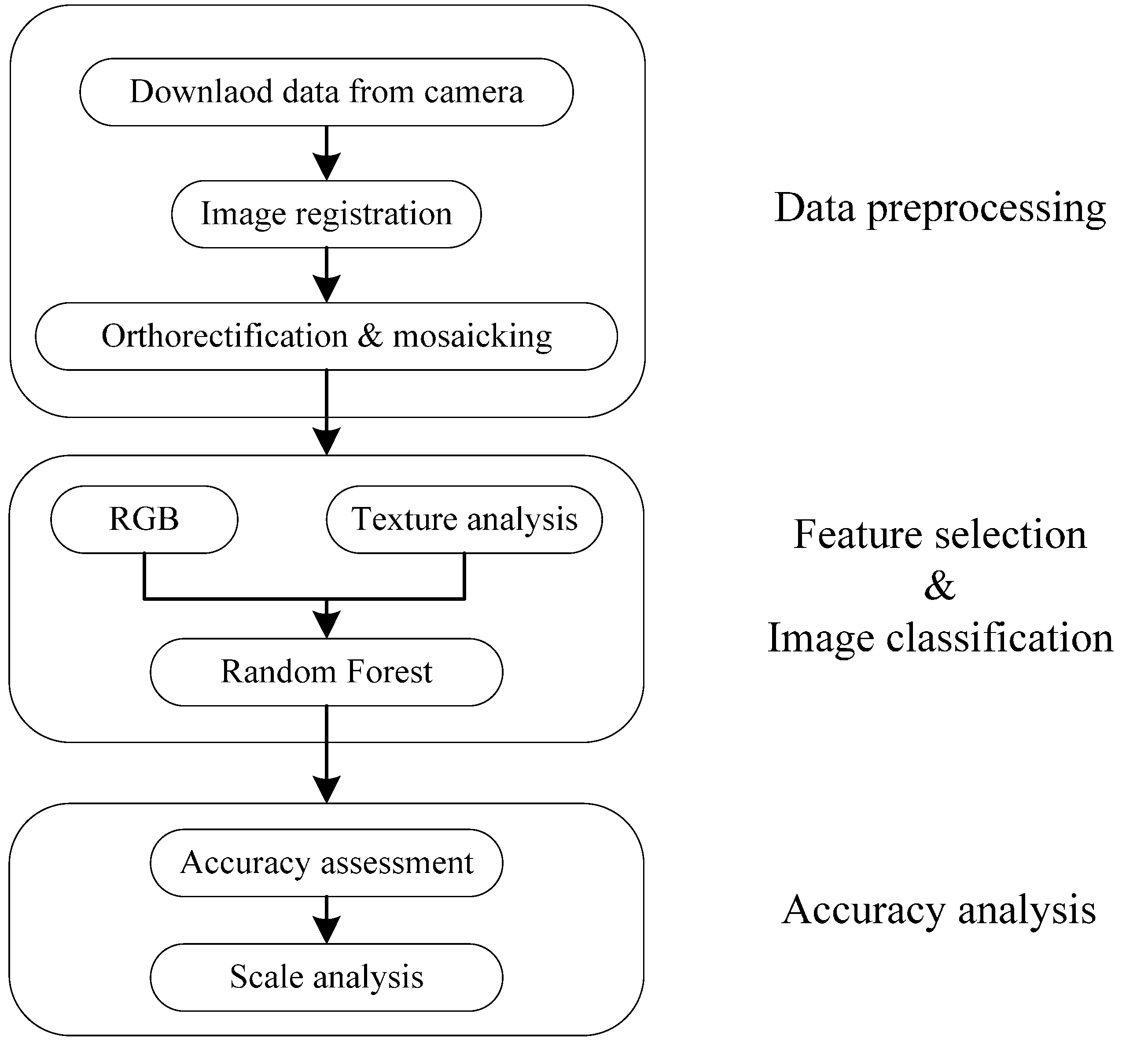
2.1. UAV Image Processing Workflow

The whole workflow of urban vegetation mapping is shown in Figure 1. It can be divided into three parts: (i) data acquisition and preprocessing; (ii) image classification; (iii) accuracy analysis. Data preprocessing was a prerequisite which involves data downloading from UAV digital camera, image registration, orthorectification and automatic mosaicking. Image classification was based on Random Forest and texture analysis. Training samples containing both RGB digital numbers and texture measures at different scales were randomly picked to train the Random Forest classifier. Accuracy assessment was done based on confusion matrix derived from validation samples to test the performance of Random Forest and the contribution of texture features at different window sizes.

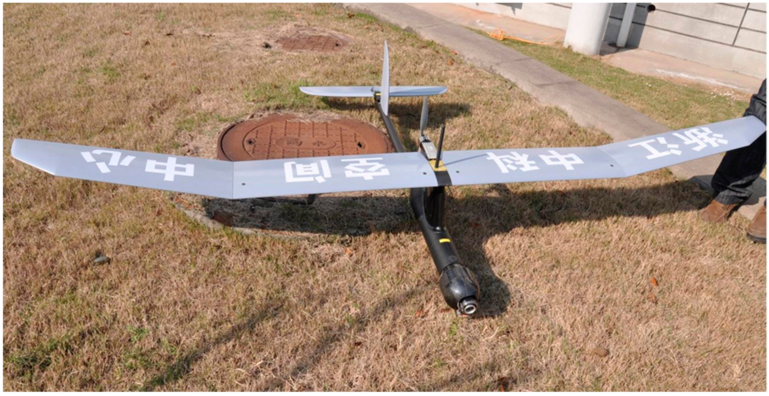
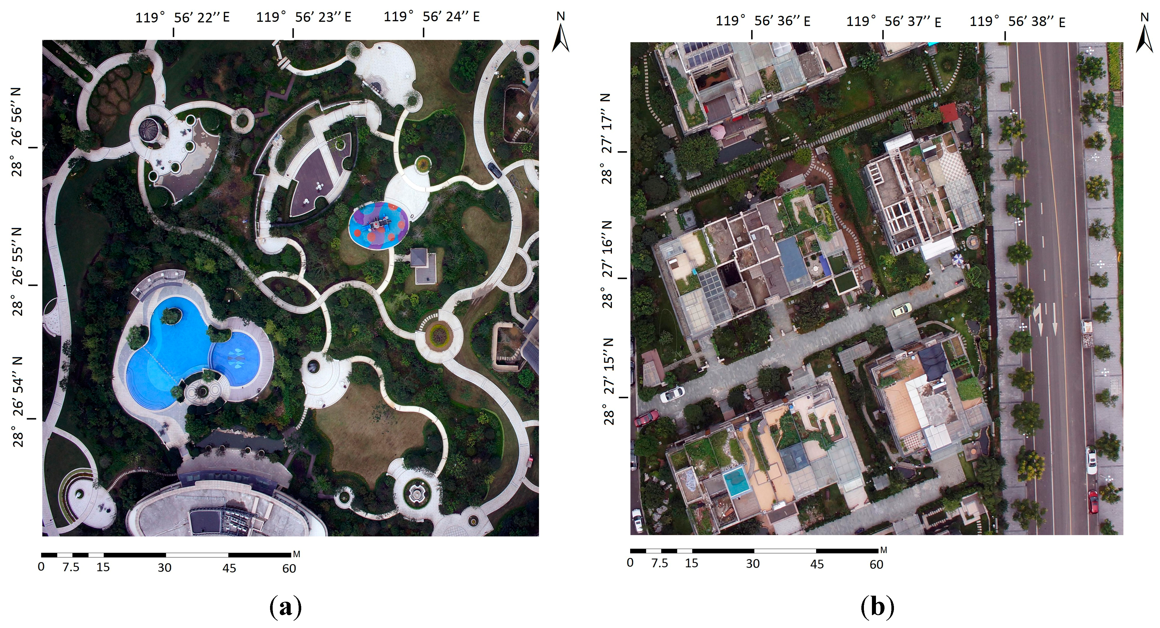
2.2. Data Acquisition and Preprocessing

The imagery was acquired with a mini-UAV called River-Map (Figure 2). The River-Map UAV system consists of sensor payload, auto pilot, GPS/INS and ground station. The UAV belongs to small sized UAVs with a wingspan of 2.5 m and a length of 1.58 m. Due to its low payload capacity, the River-Map UAV only carries a lightweight off-the-shelf digital camera onboard which acquires RGB images. The flight altitude was 200 m resulting in a resolution of 7 cm per-pixel. To satisfy the requirement of aerial photography, the forward and side overlap were set to be 60% and 30% during mission planning, respectively.

Figure 1. Workflow of urban vegetation mapping using Unmanned Aerial Vehicle (UAV) imagery.

Figure 1. Workflow of urban vegetation mapping using Unmanned Aerial Vehicle (UAV) imagery.

Figure 2. River-Map UAV.

Figure 2. River-Map UAV.

Raw images taken by the camera were orthorectified then mosaicked into a single image using Pix4D [27] with a root mean square error of 0.2 pixel. We chose Pix4D software as the preprocessing tool due to its high efficiency and good accuracy [27]. Two small images (1700 × 1700 pixels, about 120 m × 120 m) representing typical urban landscapes were chosen as test data, shown in Figure 3a,b. The images were taken in Lishui, a fast developing city in southwestern Zhejiang Province of China. Besides, the images were collected in October 2013 during the leaf-on conditions and they were provided for Lishui Urban Planning Bureau.

Figure 3. (a) A highly-vegetated recreational park; (b) A complex residential area.

Figure 3. (a) A highly-vegetated recreational park; (b) A complex residential area.

According to field survey and the aim of the project, three vegetated land covers were chosen as follows: grass, trees and shrubs. The details of these land covers acquired by UAV are shown in Figure 4. All these vegetation show similar colors but different shapes and textures. The inclusion of texture measures may help improve between-class separability hence to increase classification precision.

Figure 4. Typical urban plants. (a) Grass; (b) Trees; (c) Shrubs.

Figure 4. Typical urban plants. (a) Grass; (b) Trees; (c) Shrubs.

2.3. Texture Analysis

Texture refers to the visual effect caused by spatial variation in tonal quantity over relatively small areas [28]. Texture analysis has been widely used in remote sensing applications, especially in HR and VHR image processing [12,13,14]. The inclusion of texture can improve classification accuracy according to many studies [12,13,14,15].

Due to the limitation of payload capacity, the River-Map UAV only carried a light-weight off-the-shelf digital camera onboard. Raw images acquired were RGB ordered and JPEG formatted. The lack of a near infrared band may cause spectral confusion among different land cover types and lead to poor classification results when using per-pixel spectral-based classification methods [29]. To tackle this challenge, texture analysis was adopted because texture represents patterns in pixels that cannot be described by spectral values and individual pixels alone.

The texture statistics (e.g., mean, variance, homogeneity) used in this study were second-order (co-occurrence) textures derived from gray-level co-occurrence matrix (GLCM) which indicates the probability that values of each pair of pixels co-occur in a given direction and at certain lag distance in the image [15]. As many of the fourteen texture measures defined by Haralick [15] were correlated, the six least correlated texture measures according to Szantoi [13] were used in this study, i.e., mean (MEA), standard deviation (STD), homogeneity (HOM), dissimilarity (DIS), entropy (ENT) and angular second moment (ASM). In addition, considering that spectral bands were also highly correlated, only Green band was used for texture calculation to reduce computational burden. The texture statistics used were as follows.

$$\text{MEA}i={\displaystyle \sum _{i=0}^{N-1}{\displaystyle \sum _{j=0}^{N-1}i\times P(i,j)}}$$

(1)

$$\mathrm{STD}i=\sqrt{{\displaystyle \sum _{i=0}^{N-1}{\displaystyle \sum _{j=0}^{N-1}P(i,j)\times {(i-\mathrm{MEA}i)}^2}}}$$

(2)

$$\mathrm{HOM}={\displaystyle \sum _{i=0}^{N-1}{\displaystyle \sum _{j=0}^{N-1}\frac{P(i,j)}{1+{(i-j)}^2}}}$$

(3)

$$\mathrm{DIS}={\displaystyle \sum _{i=0}^{N-1}{\displaystyle \sum _{j=0}^{N-1}P(i,j)\times |i-j|}}$$

(4)

$$\mathrm{ENT}={\displaystyle \sum _{i=0}^{N-1}{\displaystyle \sum _{j=0}^{N-1}-P(i,j)\times \ln (P(i,j))}}$$

(5)

$$\mathrm{ASM}={\displaystyle \sum _{i=0}^{N-1}{\displaystyle \sum _{j=0}^{N-1}P{(i,j)}^2}}$$

(6)

where N is the number of grey levels; P is the normalized symmetric GLCM of dimension N × N; P(i, j) is the normalized grey level value in the cell i, j of the co-occurrence matrix such that the sum of P(i, j) equals to 1; and the calculation of texture statistics were based on a moving window around each pixel and the statistics were then attributed the pixel itself.

Generally, the bigger the window size, the coarser the information can be provided by texture features. The contribution of texture features to classification accuracy depends on both texture scale and ground objects scale. Highest accuracy can be achieved by the inclusion of the optimal scale where ground objects represent the highest between-class variation and the lowest within-class variation. To analyze how classification accuracy changes with texture window size, nine different moving windows were chosen in this study: 3 × 3 (GLCM texture 3, GT3), 5 × 5 (GT5), 7 × 7 (GT7), 9 × 9 (GT9), 11 × 11 (GT11), 15 × 15 (GT15), 21 × 21 (GT21), 31 × 31 (GT31) and 51 × 51 (GT51). Texture features derived at different window sizes were added separately as additional ancillary bands to the RGB images for further classification.

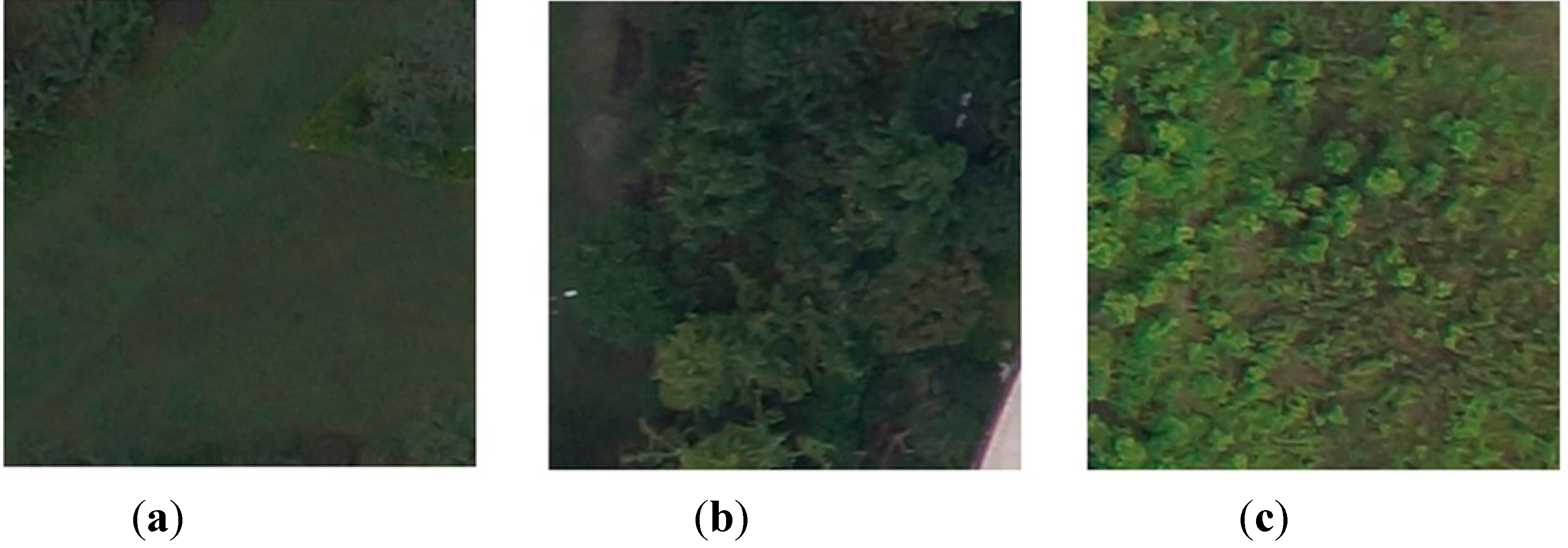
2.4. Definition of Land Cover Classes and Sampling Procedure

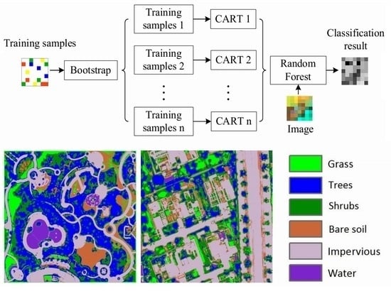
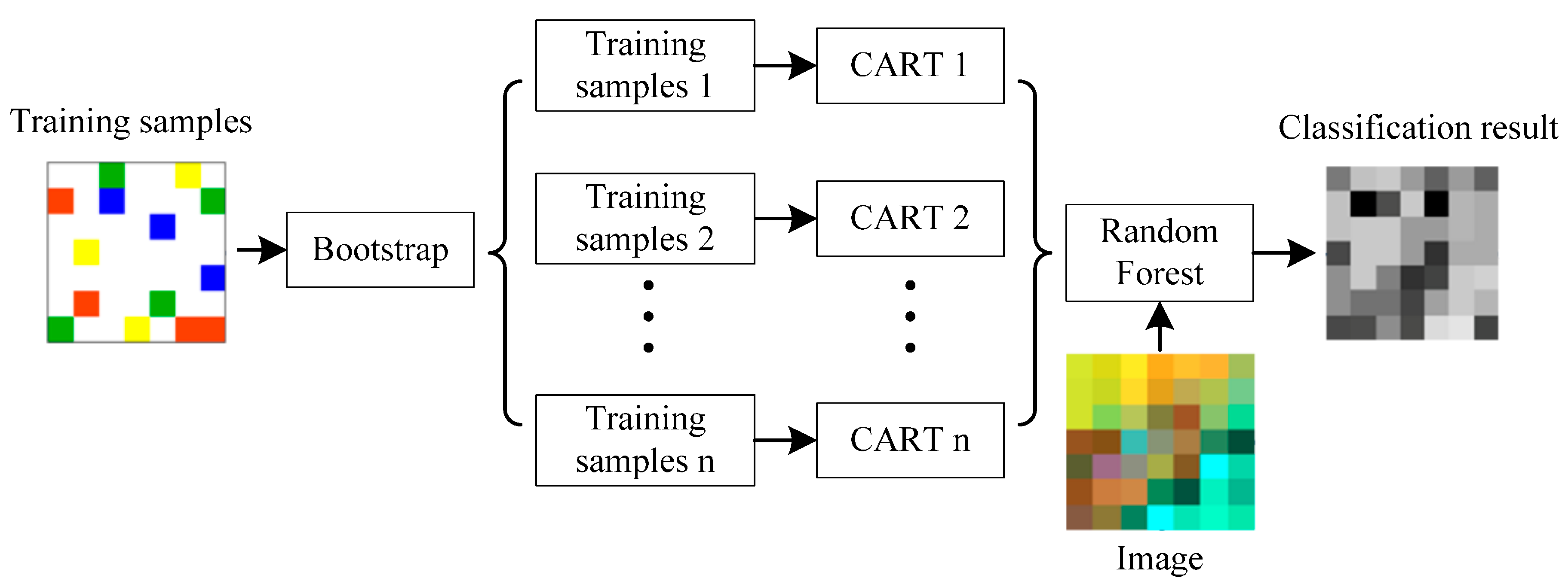
The definition of land cover classes strictly depends on the aim of the project, the study area and the resolution of the input data [30]. The aim of this study is to distinguish different land cover types over urban vegetated areas. The UHR images acquired by UAV provide the capability to distinguish trees and shrubs according to their texture differences. Based on these facts, six land cover classes were selected: grass, trees, shrubs, bare soil, water, and imperious surfaces.

The selection of training samples is very important in the supervised classification methods. Different collection strategies are available such as single pixel selection, seeding and polygon-block selection [31]. In this study, a small-block sampling procedure according to [31] was adopted. Training samples of different land covers were randomly chosen in a small polygon block. It was assumed that all pixels within each polygon belong to the same category. A total of 500 pixels were selected for each land cover class, which was enough to ensure sufficient observations.

2.5. Random Forest

Given the input data described in the previous sections, urban vegetation mapping is specified as a supervised classification of UAV orthophotos and ancillary texture features as inputs. In this study, Random Forest was used for image classification because of its robustness and efficiency. Random Forest is an ensemble learning method proposed by Breiman [18] in 2001. Compared to other machine learning methods (e.g., support vector machine, artificial neural network), there are fewer parameters to be specified when running Random Forest [18]. Meanwhile, Random Forest has been increasingly used for image classification in remote sensing fields [32,33,34,35,36,37,38,39] and can achieve equal or even higher accuracy than support vector machine [11]. Random Forest is an ensemble of many independent individual classification and regression tree (CART) and can be defined as Equation 7

$$\{h(x,{\theta }_k),k=1,\mathrm{2...}i\mathrm{...}\}$$

(7)

where h represents Random Forest classifier, x is input variable, and {θ_k} stands for independently identically distributed (i.i.d.) random predictor variables which are used for generating each CART tree [18]. The final response of Radom Forest is calculated based on the output of all the decision trees involved. The schematic diagram of Random Forest for classification is illustrated in Figure 5.

Figure 5. Schematic diagram of Random Forest for image classification.

Figure 5. Schematic diagram of Random Forest for image classification.

The creation of each decision tree that makes up the forest is the key to the success of Random Forest [18]. Two steps involving random selection are used in this process. The first step uses a bootstrap strategy [18] to randomly select about 2/3 of the training samples with replacement to build each decision tree. The remaining 1/3 samples are called out-of-bag (OOB) data [18], which are used for inner cross-validation to evaluate the classification accuracy of Random Forest. However, using only OOB errors might overestimate the performance due to over-fitting to the given training data [18], a more rigorous accuracy assessment method is always necessary such as confusion matrix derived from independent validation data. The second random sampling step is to determine the split conditions for each node in the decision tree [18]. A subset of the predictor variables is randomly selected to split each tree using Gini index [18] which is a measure of heterogeneity. The advantage of using only random selected subset of predictor variables results in less correlation among trees and a higher generalization capability. Another important advantage of Random Forest is that it can measure the importance of each input variable [18] which indicates the contribution to classification accuracy.

Random Forest only needs to specify two parameters, ntree, the number of trees to grow into a whole forest, and mty, the number of randomly selected predictor variables [37]. Generally, OOB error decreases with the increment of ntree. According to the Law of Large Numbers [37], the OOB error is convergent when ntree is bigger than a certain threshold. The plot of OOB error vs. ntree is always necessary which gives an indication whether the number of trees is sufficient in the grown forest. As for mty, a low mty means a weak prediction ability of each individual tree but a small correlation between different trees [37], which can reduce the generalization error. Two methods [37] are used to calculate mty in Random Forest, one-third or square root of the number of input variables.

Random Forest has a low computational burden, and it is insensitive to the parameters used to run it and outliers [34]. Besides, it is easy to determine which parameters to use. Over-fitting is less of an issue compared to individual decision tree and there is no need to prune the trees which is a cumbersome task [37]. All these advantages of Random Forest provide huge potential for classifying complex and texture-abundant UAV images.

2.6. Accuracy Assessment

A rigorous accuracy assessment of the proposed method for urban vegetation mapping is of great importance to verify the performance. In this study, confusion matrix was used to access the classification accuracy from independent validation samples. Kappa index, overall accuracy (OA), producer accuracy (PA) and user accuracy (UA) can be derived from confusion matrix to quantify the performance of Random Forest and the contribution of texture features to classification accuracy. Validation samples were selected independently from training samples also using the small-block sampling procedure. The number of validation samples for each class was 500, the same as training samples.

3. Results and Discussion

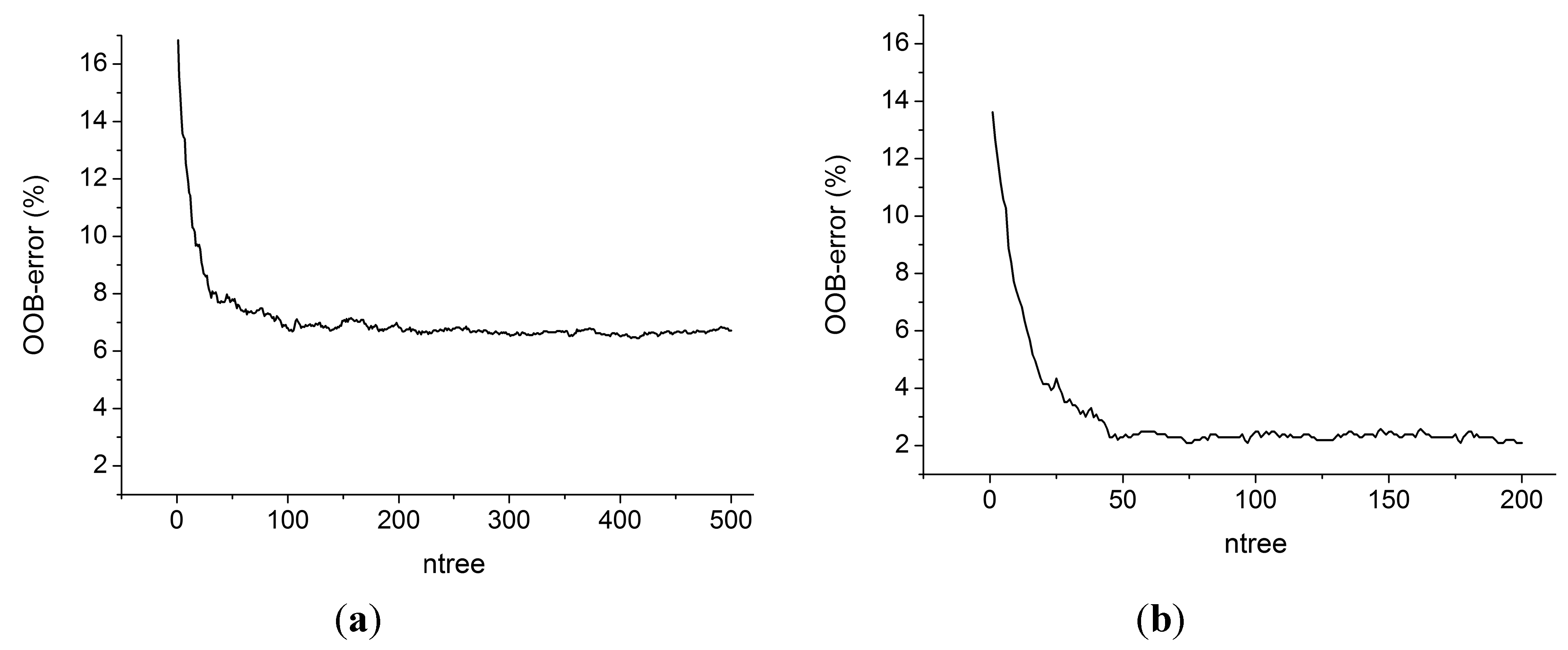
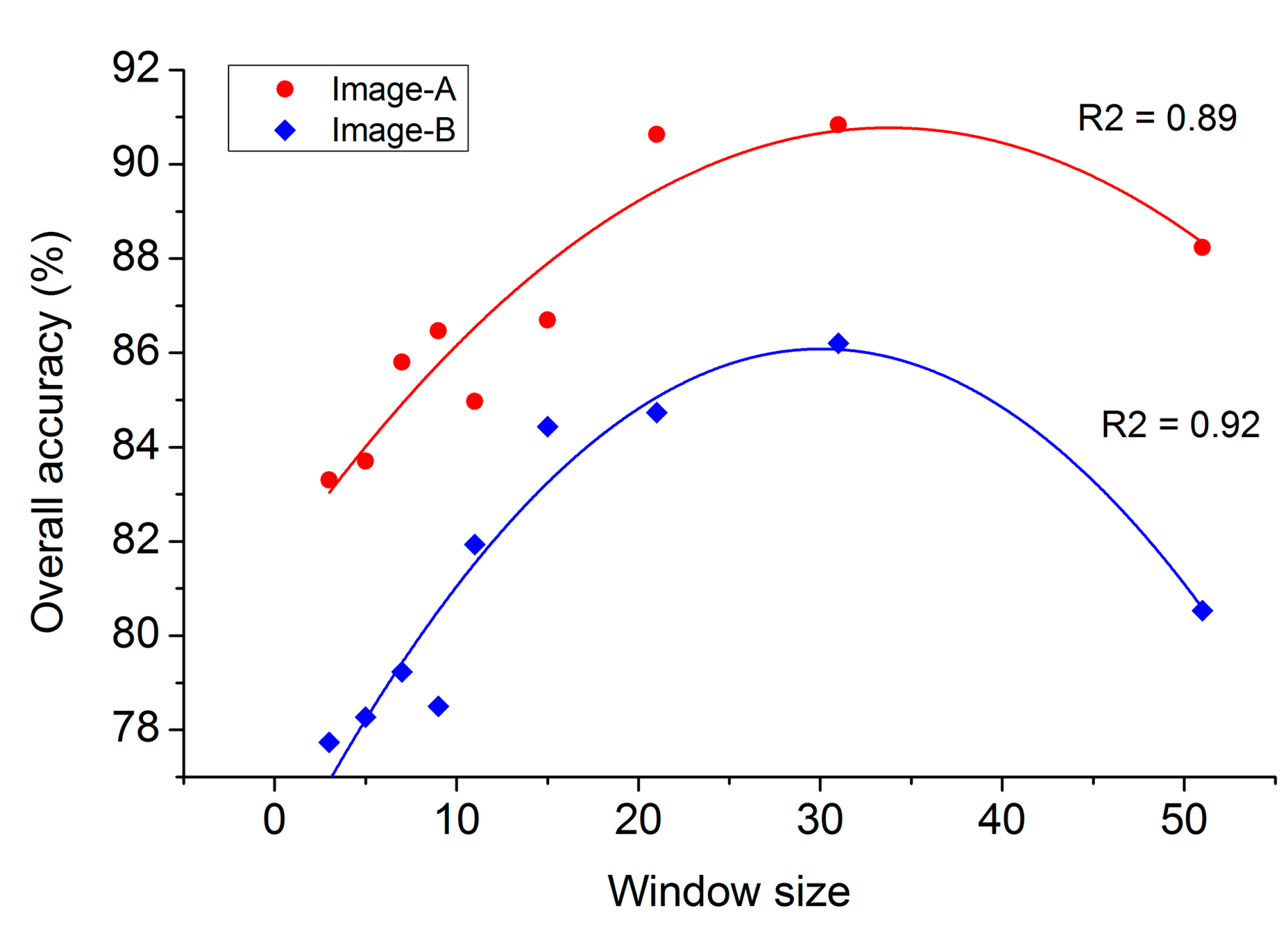
3.1. Parameterization of Random Forest

As stated above, the performance of Random Forest depends on two important parameters, ntree and mty. The image provided for Random Forest consisted of three spectral bands (e.g., RGB) and six texture bands, i.e., the number of input variables was 9, hence mty was set to be 3 (the square root of 9). As for ntree, an optimal value should be obtained when OOB error began to show convergence. More trees than the optimal value only increase the calculation burden without any contribution to accuracy improvement. To obtain the best estimation of ntree, Image-A with GT3 was classified with a relatively large value of ntree (500) to show how the OOB error changed with the number of trees. The result is shown in Figure 6a.

Figure 6. OOB error of Random Forest for Image-A uses a single window size for texture (a) GT3; (b) GT31.

Figure 6. OOB error of Random Forest for Image-A uses a single window size for texture (a) GT3; (b) GT31.

Figure 6 depicts that OOB error diminishes sharply from 17% to 8% as ntree increases from 1 to 40. OOB error decreases slowly when ntree was between 40 and 100 and fluctuates afterwards until ntree reaches about 200. OOB error stays rather stable at 6.8% when ntree is longer than 200. Hence, ntree was set to be 200 which can acquire relatively higher accuracy and reduce calculation amount at the same time. A Random Forest with 200 decision trees was employed to classify the original UAV RGB images and images added with texture features at different window sizes (GT3 to GT 51). The results indicated that the highest accuracy was achieved with the inclusion of texture metrics GT31.

Although Figure 6a indicates a number of 200 trees is sufficient for RGB+GT3, it is still necessary to validate whether OOB error shows convergence for RGB+GT31. The OOB error vs. ntree for RGB+GT31 is plotted in Figure 6b, which manifests that Random Forest is strongly convergent with 200 decision trees. Besides, the OOB error of GT31 decreases to about 2% which is lower than that of GT3 (6.8%).

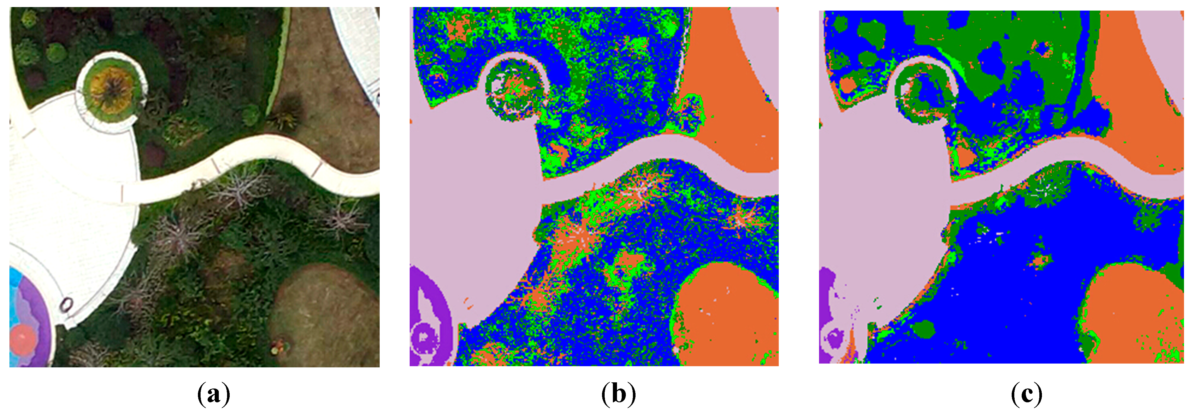
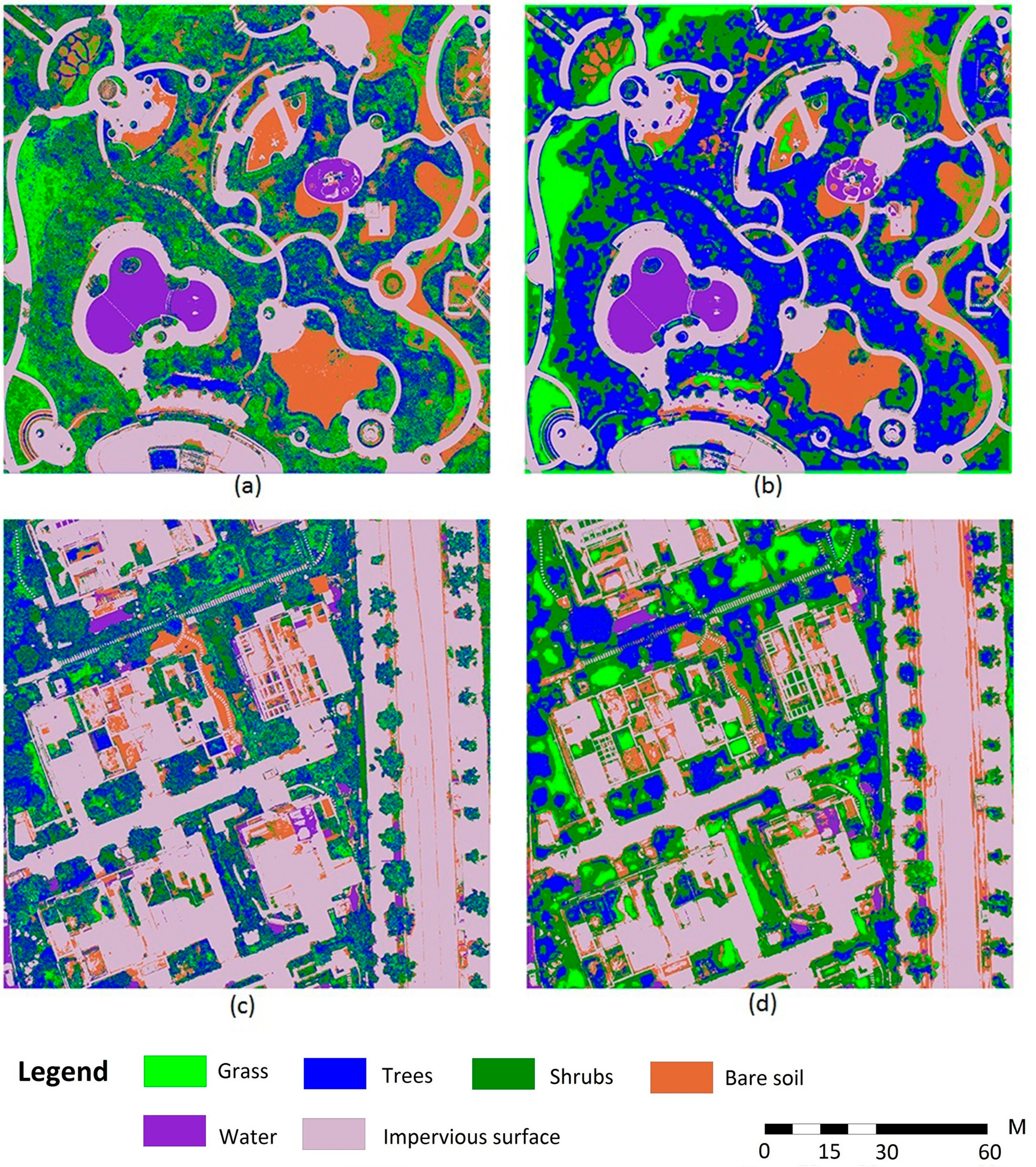
3.2. Classification Results

The trained Random Forest with 200 decision trees was adopted to classify RGB-only and RGB + texture images, resulting in the production of 10 different land-cover maps for Image-A and B, respectively. It is not possible to present all the 20 maps due to limited layout space, classification results for RGB-only and RGB+GT31 (highest accuracy) of Image-A and B are shown in Figure 7.

Figure 7 depicts the differences before and after the inclusion of texture features. When classifying RGB-only images, both Image-A and Image-B show some “salt and pepper” effects. A large amount of trees were misclassified into grass and shrubs severely. This is mainly due to the low spectral resolution of UAV images and the lack of a NIR band reduces the separability of each land cover types. However, the inclusion of texture improves the classification accuracy from a visual point of view. RGB+GT31 provided more smooth maps and an increase of tree covers substituting grass and shrubs can be clearly observed in Figure 7b,d. This is because the inclusion of texture increases the between-class separability and tends to remove small isolated groups of pixels.

Figure 7. Classification results for RGB-only and RGB+GT31 using RF. (a) Image-A RGB-only; (b) Image-A RGB+GT31; (c) Image-B RGB-only; (d) Image-B RGB+GT31.

Figure 7. Classification results for RGB-only and RGB+GT31 using RF. (a) Image-A RGB-only; (b) Image-A RGB+GT31; (c) Image-B RGB-only; (d) Image-B RGB+GT31.

To show the differences before and after the inclusion of texture features in details, one small area of the original RGB image and classification of RGB-only, RGB+GT31 is depicted as Figure 8. As can be seen in Figure 8b, some trees are misclassified as grass while some dead shrubs (without leaves) are classified as bare soil for RGB-only images. This is mainly because grass and trees, bare soil and dead shrubs share similar colors. All these misclassifications can be improved after the inclusion of six texture features at window size 31, which can be depicted in Figure 8c.

Figure 8. Details of classification result for RGB-only and RGB+GT31. (a) Original RGB image; (b) RGB-only; (c) RGB+GT31.

Figure 8. Details of classification result for RGB-only and RGB+GT31. (a) Original RGB image; (b) RGB-only; (c) RGB+GT31.

To further justify the performance of the performance of the proposed methodology, an area about 2 km² of Lishui City was tested. The image size was 28,571 × 14,286 and the processing time was about 91.24 min. The processing burden will rise with the increase of image size, and downsampling may be used to reduce the computation in practical applications. The classification result was not shown in this paper because the main focus is on the method itself and the comparison with other methods such as Maximum Likelihood and OBIA.

3.3. Results of Accuracy Assessment

To quantify the difference between classification accuracy before and after the inclusion of texture features, confusion matrix derived from 500 validation samples per class were calculated for RGB-only and RGB+GT31 images, as shown in Table 1.

Producer accuracy (PA) and user accuracy (UA) for each land cover category together with Kappa index and overall accuracy (OA) are shown in Table 1. OA for Image-A and Image-B increased from 73.5% to 90.6% and 76.6% to 86.2% respectively. The significant increment of 17.1% and 9.6% were observed to verify that the inclusion of texture features can greatly improve classification accuracy. Meanwhile, PA and UA for each land cover category in Image-A and B improved sharply after the combination of textures. In addition, when classifying RGB-only images, the errors mainly occurred among the classification of grass, trees and shrubs. This agrees with the visual inspection results of land cover maps in Figure 7. The similarity of colors among the three vegetated land covers gives rise to errors in classifying RGB-only images. The inclusion of texture increased the separability thus to increase the precision.

Table 1. Accuracy assessment of Random Forest with and without texture features.

Image-A	Ground Truth
Classes	Grass	Trees	Shrubs	Bare soil	Impervious	Water	UA (%)
Grass	461 (229)	0 (79)	3 (71)	18 (26)	12 (0)	0 (0)	93.3 (56.5)
Trees	0 (70)	456 (253)	79 (142)	0 (0)	0 (0)	0 (0)	85.2 (54.4)
Shrubs	39 (201)	44 (134)	409 (281)	25 (0)	0 (0)	0 (0)	79.1 (45.6)
Bare soil	0 (0)	0 (23)	9 (6)	457 (474)	0 (12)	22 (0)	93.7 (92.0)
Imperious	0 (0)	0 (11)	0 (0)	0 (0)	488 (488)	30 (19)	94.2 (94.2)
Water	0 (0)	0 (0)	0 (0)	0 (0)	0 (0)	448 (481)	100 (100)
PA (%)	92.2 (45.8)	91.2 (50.6)	81.8 (56.2)	91.4 (94.8)	97.6 (97.6)	89.6 (96.2)
OA (%)	90.6 (73.5)			Kappa	0.8876 (0.6824)
Image-B	Ground Truth
Classes	Grass	Trees	Shrubs	Bare soil	Impervious	Water	UA (%)
Grass	387 (268)	44 (152)	18 (45)	0 (0)	0 (0)	0 (0)	86.2 (57.6)
Trees	72 (167)	338 (246)	55 (96)	10 (0)	0 (0)	4 (3)	70.6 (48.1)
Shrubs	39 (60)	114 (101)	409 (320)	14 (13)	1 (0)	0 (1)	70.9 (64.7)
Bare soil	2 (5)	4 (1)	0 (4)	476 (481)	19 (12)	0 (2)	95.0 (95.3)
Imperious	0 (0)	0 (0)	6 (3)	0 (6)	480 (488)	0 (0)	98.8 (98.2)
Water	0 (0)	0 (0)	12 (32)	0 (0)	0 (0)	496 (494)	97.6 (93.9)
PA (%)	77.4 (53.6)	67.6 (49.2)	81.8 (64.0)	95.2 (96.2)	96.0 (97.6)	99.2 (98.8)
OA (%)	86.2 (76.6)			Kappa	0.8344 (0.7188)

Note: numbers in the brackets are the results of RGB-only images.

Table 1. Accuracy assessment of Random Forest with and without texture features.

Image-A	Ground Truth
Classes	Grass	Trees	Shrubs	Bare soil	Impervious	Water	UA (%)
Grass	461 (229)	0 (79)	3 (71)	18 (26)	12 (0)	0 (0)	93.3 (56.5)
Trees	0 (70)	456 (253)	79 (142)	0 (0)	0 (0)	0 (0)	85.2 (54.4)
Shrubs	39 (201)	44 (134)	409 (281)	25 (0)	0 (0)	0 (0)	79.1 (45.6)
Bare soil	0 (0)	0 (23)	9 (6)	457 (474)	0 (12)	22 (0)	93.7 (92.0)
Imperious	0 (0)	0 (11)	0 (0)	0 (0)	488 (488)	30 (19)	94.2 (94.2)
Water	0 (0)	0 (0)	0 (0)	0 (0)	0 (0)	448 (481)	100 (100)
PA (%)	92.2 (45.8)	91.2 (50.6)	81.8 (56.2)	91.4 (94.8)	97.6 (97.6)	89.6 (96.2)
OA (%)	90.6 (73.5)			Kappa	0.8876 (0.6824)
Image-B	Ground Truth
Classes	Grass	Trees	Shrubs	Bare soil	Impervious	Water	UA (%)
Grass	387 (268)	44 (152)	18 (45)	0 (0)	0 (0)	0 (0)	86.2 (57.6)
Trees	72 (167)	338 (246)	55 (96)	10 (0)	0 (0)	4 (3)	70.6 (48.1)
Shrubs	39 (60)	114 (101)	409 (320)	14 (13)	1 (0)	0 (1)	70.9 (64.7)
Bare soil	2 (5)	4 (1)	0 (4)	476 (481)	19 (12)	0 (2)	95.0 (95.3)
Imperious	0 (0)	0 (0)	6 (3)	0 (6)	480 (488)	0 (0)	98.8 (98.2)
Water	0 (0)	0 (0)	12 (32)	0 (0)	0 (0)	496 (494)	97.6 (93.9)
PA (%)	77.4 (53.6)	67.6 (49.2)	81.8 (64.0)	95.2 (96.2)	96.0 (97.6)	99.2 (98.8)
OA (%)	86.2 (76.6)			Kappa	0.8344 (0.7188)

Note: numbers in the brackets are the results of RGB-only images.

To analyze how the overall accuracy changes with texture scale (i.e., the size of moving window upon which texture features are derived and calculated), the curve of OA vs. texture window size is illustrated in Figure 9. A quadratic polynomial relationship between OA and texture window size is found to be significantly high, with an R-square of 0.89 and 0.92 for Image-A and Image-B, respectively.

Figure 9. Fitted curve describing how OA changes with window sizes for Image-A and B.

Figure 9. Fitted curve describing how OA changes with window sizes for Image-A and B.

Figure 9 indicates that there exits an optimal scale which assists Random Forest to achieve the highest accuracy. With the enlargement of texture window size, the accuracy increases to the highest until the optimal texture scale is reached. Once the texture window size surpasses the optimal value, the accuracy begins to fall first gradually and then sharply. The optimal texture window size for Image-A and B are both 31. As the UAV image has a ground resolution of 7 cm, the actual size for GT31 is 2.17 m. The field survey indicated that 2.17 m is in accordance with the average crown size of shrubs, under which the differences among grass, shrubs and trees are maximized. However, from a universality perspective, it might be difficult to determine the optimal scale through a formula. It may take some time to do a series of experiments and this is a drawback of the proposed method.

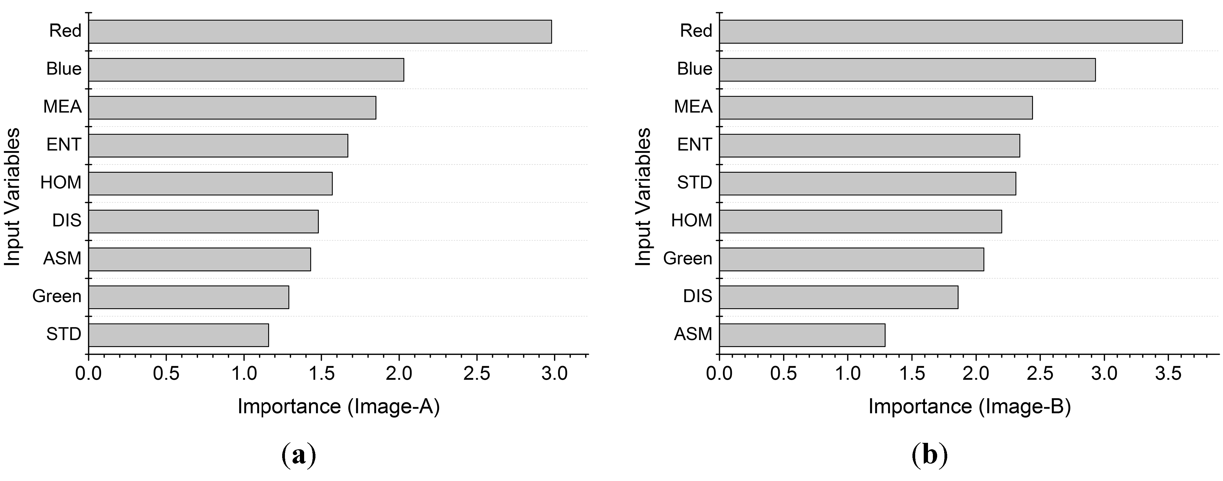
3.4. Variable Importance

The importance of input variables given by Random Forest can be used to measure their contribution to classification accuracy. The importance of the input variables is depicted in Figure 10.

Figure 10. Importance of input variables. (a) Image-A; (b) Image-B.

Figure 10. Importance of input variables. (a) Image-A; (b) Image-B.

It can be seen from Figure 10 that the four most important variables are the same for both Image-A and B: Red band, Blue band, MEA and ENT. Green band has a much lower importance than that of Red and Blue band, which is mainly because trees, grass and shrubs manifest the similar green color. MEA is the most important variable since the mean value can decrease the random error. ENT ranks the second among texture features due to its capability in capturing the spatial distribution characteristics of different land covers. On the whole, Red and Blue bands are more important than all the texture features which indicates that although the inclusion of texture can increase classification precision of Random Forest classifier, spectral features remain the most important variables in urban vegetation mapping.

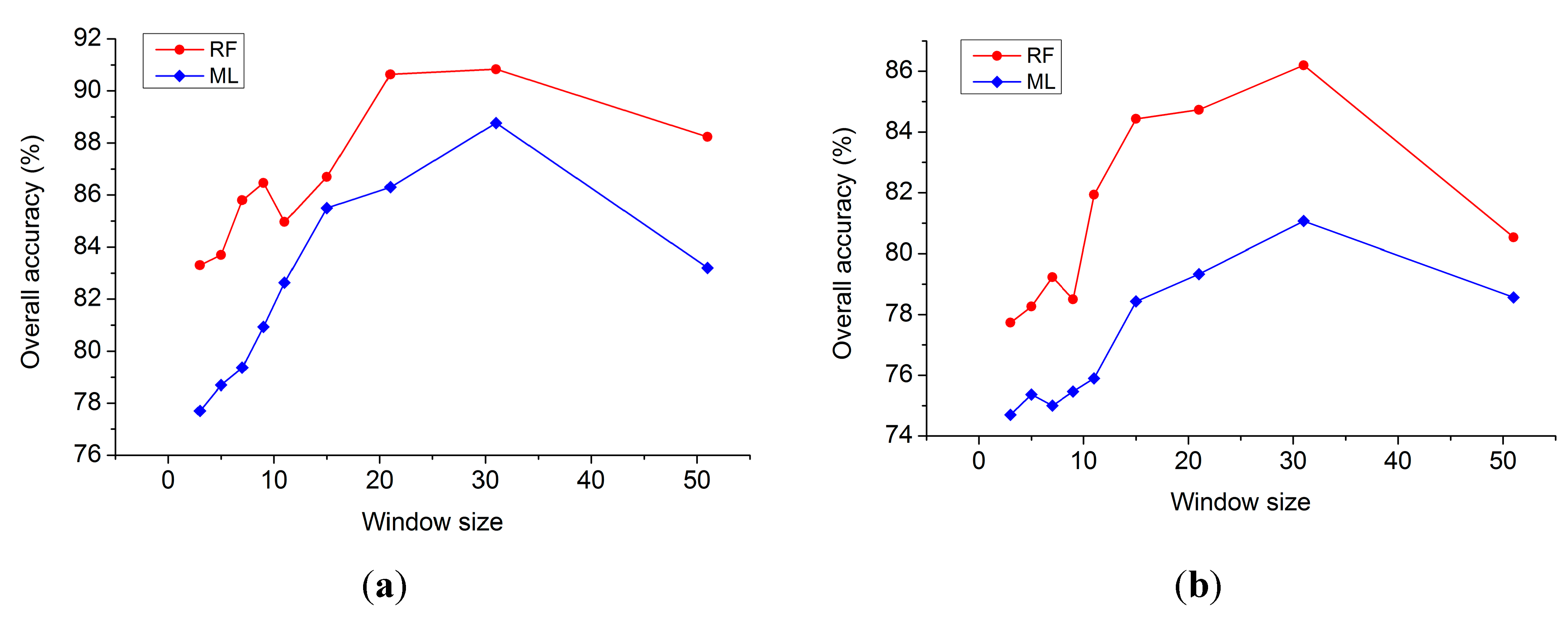
3.5. Comparison with Maximum Likelihood

To verify the performance of Random Forest in urban vegetation mapping, Maximum Likelihood classifier was used as a benchmark due to its importance in remote sensing applications. The formulas used for ML are described explicitly in many studies [40] and they are not repeated here. Image-A and B with the inclusion of all the texture features (GT3 to GT51) were classified by ML separately using the same training samples. Accuracy assessment was done through confusion matrix derived from the same validation samples. The comparison of overall accuracy between RF and ML is described in Figure 11.

Figure 11. Accuracy comparison between Random Forest and Maximum Likelihood. (a) Image-A; (b) Image-B.

Figure 11. Accuracy comparison between Random Forest and Maximum Likelihood. (a) Image-A; (b) Image-B.

Figure 11 shows that Random Forest classifier outperforms traditional ML method under each texture scale for both Image-A and Image-B. The maximum of OA increase for Image-A and B is 6.43% achieved at scale GT7, and 6.03% at GT11. OA increased averagely 3.94% and 4.12% for Image-A and B by using Random Forest. Besides, OA curves of ML shows similar patterns as those of RF, and the optimal texture window size is still 31 for both Image-A and B, which verify that scale effect exists regardless of different classifiers.

ML is a parametric algorithm and assumes that input variables are normally distributed [41]. However, this assumption is always violated when dealing with real data, which results in the limitation of ML. Unlike ML, RF does not need this assumption. The ensemble learning mechanism of RF guarantees the good performance regardless of the distribution pattern [18], which interprets why RF outperformed ML under every texture window size.

3.6. Comparison with OBIA

The comparison results in 3.6 only verified that Random Forest outperformed the traditional Maximum Likelihood classifier. However, it is still quite necessary to compare the proposed method (RF + Texture) in this study with the state-of-art method, OBIA, to further justify its performance in urban vegetation mapping.

In order to carry out OBIA, Feature Extraction (FX) with Example-Based Classification in ENVI 5.1 [42] was adopted to classify Image-A and B. The entire process can be divided into four parts: (i) image segmentation; (ii) feature selection; (iii) image classification; and (iv) precision assessment. Firstly, Edge segmentation method [43] was used to divide the image into segments and Full Lambda Schedule merging method [43] was employed to combine adjacent segments. Scale Level (0–100) and Merge Level (0–100) [43] should be optimized at the same time to obtain the best segmentation results. A higher Scale Level indicates bigger segments while a higher Merge Level means more adjacent segments will be combined together [43]. Secondly, various spatial, spectral and texture features were computed for each segment. A total of 38 features were selected such as Area, Roundness, Spectral Min, Texture Entropy and so on [43]. Thirdly, a supervised classification method should be used based on training samples to classify the image. Three methods are provided here by FX, i.e., K Nearest Neighbor (KNN), Support Vector Machine (SVM) and Principle Component Analysis (PCA) [43]. SVM was selected because it is the most rigorous method among the three classification methods. Radial Basis [43] was selected as kernel function of SVM due to its efficiency. Gamma in kernel function [43] was set to be 0.026, which was the inverse of the number of input variables. Penalty parameter [43] was set to be 100 as default. Finally, accuracy assessment was done based on both confusion matrix and visual inspection.

A number of classification experiments were done base on SVM with different Scale and Merge Level and results indicated that a Scale Level of 30 and a Merge Level of 20 yielded the highest overall accuracy. The classification results of Image-A and B are shown in Figure 12.

Figure 12. Classification results using OBIA. (a) Image-A; (b) Image-B.

Figure 12. Classification results using OBIA. (a) Image-A; (b) Image-B.

From a visual inspection, the drawback of “salt and pepper” effects in pixel-based methods were mostly eliminated in Figure 12 because OBIA treated the image based on small segments rather than individual pixels. Besides, the results of OBIA were very similar to that of RF + Texture when comparing Figure 12 to Figure 7, which indicates that the proposed method in this study can achieve similar performance to OBIA from a visual point of view. Nevertheless, it is highly necessary to compare the two methods quantitatively. Confusion matrix for OBIA results were derived from the same validation samples as that of RF + Texture and a comprehensive comparison of the two methods was shown in the following table.

Table 2 shows that RF + Texture is slightly inferior to OBIA in terms of overall accuracy and Kappa index. This is not surprising since OBIA used much more features than RF + Texture for classification. Besides, SVM, one of the best statistic learning theories was utilized in OBIA to achieve high precision. However, RF + Texture still yielded good performance. Processing burden is lighter because only nine features were used instead of numerous spatial, spectral and texture features in OBIA. Since texture features are capable of capturing the contextual relationship between pixels, RF + Texture can significantly remove the salt and pepper noise hence to generate more smooth maps, which shows quite similar results as OBIA. Besides, RF + Texture does not require image segmentation and merging whose Scale Level and Merge Level need to be optimized using many experiments. Although RF + Texture needs to find the optimal window size for texture statistics, it is still simpler to carry out than optimizing the two parameters (Scale and Merge Level) at the same time. Last but not least, the parameterization of RF is simpler and easier to carry out than SVM while the latter requires experiments to specify the kernel function type, punishment coefficient and Gamma in kernel function simultaneously. Taking all these issues into consideration, the proposed RF + Texture method can be viewed as a simplified version of OBIA, which is independent on image segmentation and numerous image features and can yet achieve similar performance as OBIA.

Table 2. Comparison of OBIA and RF + Texture.

Image	Method	Feature Used	OA (%)	Kappa	Time (s)
Image-A	OBIA	38	91.8	0.9016	63.8
	RF + Texture	9	90.6	0.8876	41.2
Image-B	OBIA	38	88.1	0.8572	53.1
	RF + Texture	9	86.2	0.8344	34.5

Table 2. Comparison of OBIA and RF + Texture.

Image	Method	Feature Used	OA (%)	Kappa	Time (s)
Image-A	OBIA	38	91.8	0.9016	63.8
	RF + Texture	9	90.6	0.8876	41.2
Image-B	OBIA	38	88.1	0.8572	53.1
	RF + Texture	9	86.2	0.8344	34.5

4. Conclusions

This paper proposed an accurate hybrid method via combining Random Forest and texture analysis for vegetation mapping in heterogeneous urban landscapes based on UAV remote sensing. The ultra-high resolution images (7 cm) acquired by UAV provide sufficient details for urban vegetation extraction. Six least correlated GLCM texture features were calculated and added to the original RGB image to construct a multi-dimensional spectral-texture feature space. A Random Forest consisting of 200 trees was used to classify two selected UAV orthophotos in typical urban landscapes. Experimental results showed that overall accuracy for Image-A and Image-B increased from 73.5% to 90.6% and 76.6% to 86.2% after the inclusion of texture features, respectively, which indicated that texture plays a significant role in improving classification accuracy. The impact of texture window size on classification accuracy was also analyzed in this paper, and an inverted U relationship was observed between overall accuracy and texture window size. Besides, when using Random Forest instead of Maximum Likelihood, overall accuracy increased by about 4% in average indicating that RF outperformed ML under each texture scale. When comparing RF + Texture to the state-of-art method OBIA, the latter yielded a slightly higher accuracy (an increase of 1.5%) but at the cost of computation burden. In summary, RF outperformed ML and showed similar performance to OBIA.

This paper demonstrates that UAV is an outstanding platform for urban vegetation monitoring. The hybrid method can provide accurate classification results to reduce the drawbacks of off-the-shelf digital cameras. However, cameras incorporating a NIR band should be used for serious data acquisition in future works and validation of the proposed method should be extended to images from different areas and different time of the year. The comparison between the proposed method and the smoothed version of pure RGB classification results should be conducted. Finally, the uncertainty analysis of the proposed method should also be considered.

References

1. Nichol, J.; Lee, C.M. Urban vegetation monitoring in Hong Kong using high resolution multispectral images. Int. J. Remote Sens. 2005, 26, 903–918. [Google Scholar] [CrossRef]
2. Small, C. Estimation of urban vegetation abundance by spectral mixture analysis. Int. J. Remote Sens. 2001, 22, 1305–1334. [Google Scholar] [CrossRef]
3. Zhang, X.; Feng, X.; Jiang, H. Object-oriented method for urban vegetation mapping using IKONOS imagery. Int. J. Remote Sens. 2010, 31, 177–196. [Google Scholar] [CrossRef]
4. Tigges, J.; Lakes, T.; Hostert, P. Urban vegetation classification: Benefits of multitemporal RapidEye satellite data. Remote Sens. Environ. 2013, 136, 66–75. [Google Scholar] [CrossRef]
5. Alonzo, M.; Bookhagen, B.; Roberts, D.A. Urban tree species mapping using hyperspectral and LiDAR data fusion. Remote Sens. Environ. 2014, 148, 70–83. [Google Scholar] [CrossRef]
6. Tooke, T.R.; Coops, N.C.; Goodwin, N.R.; Voogt, J.A. Extracting urban vegetation characteristics using spectral mixture analysis and decision tree classifications. Remote Sens. Environ. 2009, 113, 398–407. [Google Scholar] [CrossRef]
7. Li, X.; Shao, G. Object-based urban vegetation mapping with high-resolution aerial photography as a single data source. Int. J. Remote Sens. 2013, 34, 771–789. [Google Scholar] [CrossRef]
8. Johansen, K.; Coops, N.C.; Gergel, S.E.; Stange, Y. Application of high spatial resolution satellite imagery for riparian and forest ecosystem classification. Remote Sens. Environ. 2007, 110, 29–44. [Google Scholar] [CrossRef]
9. Höfle, B.; Hollaus, M.; Hagenauer, J. Urban vegetation detection using radiometrically calibrated small-footprint full-waveform airborne LiDAR data. ISPRS J. Photogramm. Remote Sens. 2012, 67, 134–147. [Google Scholar] [CrossRef]
10. Powell, R.L.; Roberts, D.A.; Dennison, P.E.; Hess, L.L. Sub-pixel mapping of urban land cover using multiple endmember spectral mixture analysis: Manaus, Brazil. Remote Sens. Environ. 2007, 106, 253–267. [Google Scholar] [CrossRef]
11. Rosa, D.L.; Wiesmann, D. Land cover and impervious surface extraction using parametric and non-parametric algorithms from the open-source software R: An application to sustainable urban planning in Sicily. GISci. Remote Sens. 2013, 50, 231–250. [Google Scholar]
12. Laliberte, A.S.; Rango, A. Texture and scale in object-based analysis of subdecimeter resolution Unmanned Aerial Vehicle (UAV) imagery. IEEE Trans. Geosci. Remote Sens. 2009, 47, 761–770. [Google Scholar] [CrossRef]
13. Szantoi, Z.; Escobedo, F.; Abd-Elrahman, A.; Smith, S.; Pearlstine, L. Analyzing fine-scale wetland composition using high resolution imagery and texture features. Int. J. Appl. Earth Obs. 2013, 23, 204–212. [Google Scholar] [CrossRef]
14. Aguera, F.; Aguilar, F.J.; Aguilar, M.A. Using texture analysis to improve per-pixel classification of very high resolution images for mapping plastic greenhouses. ISPRS J. Photogramm. Remote Sens. 2008, 63, 635–646. [Google Scholar] [CrossRef]
15. Haralick, R.M.; Dinstein, I.; Shanmugam, K. Textural features for image classification. IEEE Trans. Syst. Man Cybern. 1973, 3, 610–621. [Google Scholar] [CrossRef]
16. Cleve, C.; Kelly, M.; Kearns, M.R.; Moritz, M. Classification of the wildland–urban interface: A comparison of pixel- and object-based classifications using high-resolution aerial photography. Comput. Environ. Urban Syst. 2008, 32, 317–326. [Google Scholar] [CrossRef]
17. Yu, Q.; Gong, P.; Clinton, N.; Biging, G.; Kelly, M.; Schirokauer, D. Object-based detailed vegetation classification with airborne high spatial resolution remote sensing imagery. Photogramm. Eng. Remote Sens. 2006, 72, 799–811. [Google Scholar] [CrossRef]
18. Breiman, L. Random forests. Mach. Learn. 2001, 45, 5–32. [Google Scholar] [CrossRef]
19. Laliberte, A.S.; Goforth, M.A.; Steele, C.M.; Rango, A. Multispectral remote sensing from unmanned aircraft: Image processing workflows and applications for rangeland environments. Remote Sens. 2011, 3, 2529–2551. [Google Scholar] [CrossRef]
20. Qin, R. An object-based hierarchical method for change detection using unmanned aerial vehicle images. Remote Sens. 2014, 6, 7911–7932. [Google Scholar] [CrossRef]
21. Honkavaara, E.; Saari, H.; Kaivosoja, J.; Pölönen, I.; Hakala, T.; Litkey, P.; Mäkynen, J.; Pesonen, L. Processing and assessment of spectrometric, stereoscopic imagery collected using a lightweight UAV spectral camera for precision agriculture. Remote Sens. 2013, 5, 5006–5039. [Google Scholar] [CrossRef] [Green Version]
22. Wallace, L.; Lucieer, A.; Watson, C.; Turner, D. Development of a UAV-LiDAR system with application to forest inventory. Remote Sens. 2012, 4, 1519–1543. [Google Scholar] [CrossRef]
23. Hunt, E.R.; Hively, W.D.; Fujikawa, S.J.; Linden, D.S.; Daughtry, C.S.T.; McCarty, G.W. Acquisition of NIR-Green-Blue digital photographs from unmanned aircraft for crop monitoring. Remote Sens. 2010, 2, 290–305. [Google Scholar] [CrossRef]
24. Rango, A.; Laliberte, A.; Herrick, J.E.; Winters, C.; Havstad, K.; Steele, C.; Browning, D. Unmanned aerial vehicle-based remote sensing for rangeland assessment, monitoring, and management. J. Appl. Remote Sens. 2009, 3, 1–15. [Google Scholar]
25. Gong, J.; Yue, Y.; Zhu, J.; Wen, Y.; Li, Y.; Zhou, J.; Wang, D.; Yu, C. Impacts of the Wenchuan Earthquake on the Chaping River upstream channel change. Int. J. Remote Sens. 2012, 33, 3907–3929. [Google Scholar] [CrossRef]
26. Colomina, I.; Molina, P. Unmanned aerial systems for photogrammetry and remote sensing: A review. ISPRS J. Photogramm. Remote Sens. 2014, 92, 79–97. [Google Scholar] [CrossRef]
27. Pix4D. Available online: http://pix4d.com (accessed on 31, October, 2014).
28. Anys, H.; He, D.C. Evaluation of textural and multipolarization radar features for crop classification. IEEE Trans. Geosci. Remote Sens. 1995, 33, 1170–1181. [Google Scholar] [CrossRef]
29. Lu, D.; Hetrick, S.; Moran, E. Land cover classification in a complex urban-rural landscape with QuickBird imagery. Photogramm. Eng. Remote Sens. 2010, 76, 1159–1168. [Google Scholar] [CrossRef]
30. Lu, D.; Weng, Q. A survey of image classification methods and techniques for improving classification performance. Int. J. Remote Sens. 2007, 28, 823–870. [Google Scholar] [CrossRef]
31. Chen, D.; Stow, D. The effect of training strategies on supervised classification at different spatial resolutions. Photogramm. Eng. Remote Sens. 2002, 68, 1155–1162. [Google Scholar]
32. Rodriguez-Galiano, V.F.; Chica-Olmo, M.; Abarca-Hernandez, F.; Atkinson, P.M.; Jeganathan, C. Random forest classification of mediterranean land cover using multi-seasonal imagery and multi-seasonal texture. Remote Sens. Environ. 2012, 121, 93–107. [Google Scholar] [CrossRef]
33. Ghosh, A.; Sharma, R.; Joshi, P.K. Random forest classification of urban landscape using Landsat archive and ancillary data: Combining seasonal maps with decision level fusion. Appl. Geol. 2014, 48, 31–41. [Google Scholar] [CrossRef]
34. Puissant, A.; Rougier, S.; Stumpf, A. Object-oriented mapping of urban trees using random forest classifiers. Int. J. Appl. Earth Obs. 2014, 26, 235–245. [Google Scholar] [CrossRef]
35. Mishra, N.B.; Crews, K.A. Mapping vegetation morphology types in a dry savanna ecosystem: Integrating hierarchical object-based image analysis with random forest. Int. J. Remote Sens. 2014, 35, 1175–1198. [Google Scholar] [CrossRef]
36. Hayes, M.H.; Miller, S.N.; Murphy, M.A. High-resolution land cover classification using random forest. Remote Sens. Lett. 2014, 5, 112–121. [Google Scholar] [CrossRef]
37. Rodriguez-Galiano, V.F.; Ghimire, B.; Chica-Olmo, M.; Rigol-Sanchez, J.P. An assessment of the effectiveness of a random forest classifier for land-cover classification. ISPRS J. Photogramm. Remote Sens. 2012, 67, 93–104. [Google Scholar] [CrossRef]
38. Xu, L.; Li, J.; Brenning, A. A comparative study of different classification techniques for marine oil spill identification using RADARSAT-1 imagery. Remote Sens. Environ. 2014, 141, 14–23. [Google Scholar] [CrossRef]
39. Immitzer, M.; Atzberger, C.; Koukal, T. Tree species classification with random forest using very high spatial resolution 8-band WorldView-2 satellite data. Remote Sens. 2012, 4, 2661–2693. [Google Scholar] [CrossRef]
40. Paola, J.; Schowengerdt, R. A detailed comparison of backpropagation neural network and maximum-likelihood classifiers for urban land use classification. IEEE Trans. Geosci. Remote Sens. 1995, 33, 981–996. [Google Scholar] [CrossRef]
41. Amini, J. A method for generating floodplain maps using IKONOS images and DEMs. Int. J. Remote Sens. 2010, 31, 2441–2456. [Google Scholar] [CrossRef]
42. EXELIS. Available online: http://www.exelisvis.com/ProductsServices/ENVIProducts.aspx (accessed on 31 October 2014).
43. Feature Extraction with Example-Based Classification Tutorial. Available online: http://www.exelisvis.com/docs/FXExampleBasedTutorial.html (accessed on 31 October 2014).