The Impact of Positional Errors on Soft Classification Accuracy Assessment: A Simulation Analysis

Abstract

Validating or accessing the accuracy of soft classification maps has rapidly developed over the past few years. This assessment employs a soft error matrix as generalized from the traditional, hard classification error matrix. However, the impact of positional error on the soft classification is uncertain and whether the well-accepted half-pixel registration accuracy is suitable for the soft classification accuracy assessment is unknown. In this paper, a simulation analysis was conducted to examine the influence of positional error on the overall accuracy (OA) and kappa in soft classification accuracy assessment under different landscape conditions (i.e., spatial characteristics and spatial resolutions). Results showed that with positional error ranging from 0 to 3 soft pixels, the OA-error varied from 0 to 44.6 percent while the kappa-error varied from 0 to 93.7 percent. Landscape conditions with smaller mean patch size (MPS) and greater fragmentation produced greater positional error impact on the accuracy measures at spatial resolutions of 1 and 2 unit distances. However, this trend did not hold for spatial resolutions of 5 and 10 unit distances. A half of a pixel was not sufficient to keep the overall accuracy error and kappa error under 10 percent. The results indicate that for soft classification accuracy assessment the requirement for registration accuracy is higher and depends greatly on the landscape characteristics. There is a great need to consider positional error for validating soft classification maps of different spatial resolutions.

1. Introduction

In the past few decades, earth observation satellites (EOS) have provided large amounts of remotely sensed data depicting the earth’s surface at a variety of spatial and temporal scales. Global or regional land cover maps from these remotely sensed data are typically based on image classification and a great number of classification methods have been developed, ranging from classical ones such as minimum distance [1] to more advanced ones such as support vector machine [2]. Generally, two groups of classification methods exist: per-pixel (hard) and sub-pixel (soft) classification [3]. The hard classification methods classify the remotely sensed data into maps where each pixel belongs to a single land cover/vegetation/thematic class, whereas the soft classification methods categorize each pixel into several classes simultaneously [3]. Soft classification methods have recently gained wider use because of their ability to continuously represent and estimate the area of land cover at the sub-pixel level, especially for land cover mapping using coarse resolution data where mixed pixels dominate.

Accordingly, as an indispensable part of the classification process, there is a great need to develop methods for validating or accessing the accuracy of soft classification maps because the error matrix developed for hard classification accuracy assessment [4] may not be appropriate for use in representing the soft classification accuracy [5]. The major issue is that accuracy information will be lost if the Boolean operator typically used in a conventional error matrix to record the attribute in the reference sample unit as 1 for “correct” and 0 for “wrong” is used when determining the accuracy of a soft classification map [5]. In other words, the entire pixel is no longer either right or wrong, but rather soft classification labels parts of the pixel into different classes. Given this issue, much effort has been made to generalize the conventional error matrix and adapt it for use in soft classification. Until now, various approaches have been advanced for the sub-pixel error matrix based on a number of mathematical theories such as minimum operator [5], multiplication operator [6] and composite operator [7,8]. From the soft error matrix, a number of descriptive and analytical statistical measures can be calculated including overall accuracy (oa), kappa coefficient (kappa), user’s accuracy (ua) and producer’s accuracy (pa) [4]. It is worth noting that all these methods for constructing the soft error matrix were developed under the assumption that the classified map is perfectly co-registered between the reference data and the ground. However, in practice, no map is free of positional errors and the assessment of thematic accuracy must include or incorporate some measure of positional accuracy [9,10,11].

Positional error is regarded as one of the great sources of uncertainty in accuracy assessment [12,13,14]. Positional errors mainly arise from the geometric distortion of the image, including earth rotation effects, scanning system, and the random spacecraft movement [15], which take on different forms of distortion such as scaling, rotation, translation and scan skewing [16]. Image registration includes two steps to correct these issues. The first is called systematic correction using ephemeris data from the spacecraft and results in approximate image coordinates. The second step is precision correction which registers the image to a series of ground features by using ground control points. For accuracy assessment, the positional error between the classification map and the reference data is not limited only to image registration, but is also subject to GPS error [17] because the ground reference data are often collected using a GPS receiver. The synchronization error between the satellite and the code-phased GPS receiver results in a locational error ranging from 5 to 20 meters [18]. The assumption therefore, is that the difference between the classification map and reference data results only from the classification error not being satisfied. However, the non-thematic errors arising from misregistration can be a significant contribution to the error matrix that may then mask the real thematic accuracy information. Powell et al. [19] determined that more than 30% of thematic errors for Landsat TM could be attributed to the positional errors. This issue is more severe in heterogeneous landscapes where several map classes are located together [11]. Intuitively, for soft classification, coarser spatial resolution increases the number of mixed pixels in the classification maps [20], making the soft error matrix more sensitive to positional errors because even a slight location error between the classification and the reference map can substantially change the proportion of map classes within that mixed pixel.

Higher resolution images are often widely accepted as a substitute for the ground reference data used in validating the classification map. A half-pixel registration accuracy between the classification map and the reference map has often been reported [21] and accepted as common, especially for moderate resolution imagery such as Landsat Thematic Mapper imagery. However, whether this requirement holds for soft classification accuracy assessment and whether it changes with the varied spatial resolutions is still unknown.

Many projects have been conducted in the area of land cover dynamics, e.g., map comparison for change detection analysis. It has been shown that a slight location error can result in a great impact on the accuracy of change detection [16,22,23] and that a registration accuracy of 0.2 pixels is required to guarantee the error of change detection is less than 10% [16,24]. It was also found that the effect of positional error is influenced by the heterogeneity of the land cover. The more fragmented land cover maps produce the greater effect on the change detection error owing to positional error [25]. Aggregation-based or object-based change detection methods have been suggested to reduce the impact of the position on the change detection accuracy [26,27,28,29]. Studies of misresgistration issues in change detection analysis and soft classification have therefore provided the impetus for this paper. These issues include modeling the analysis of positional error and the study of the spatial characteristics of the land cover.

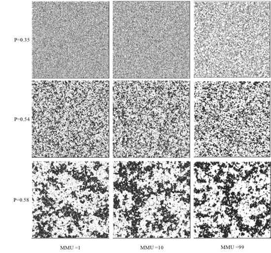
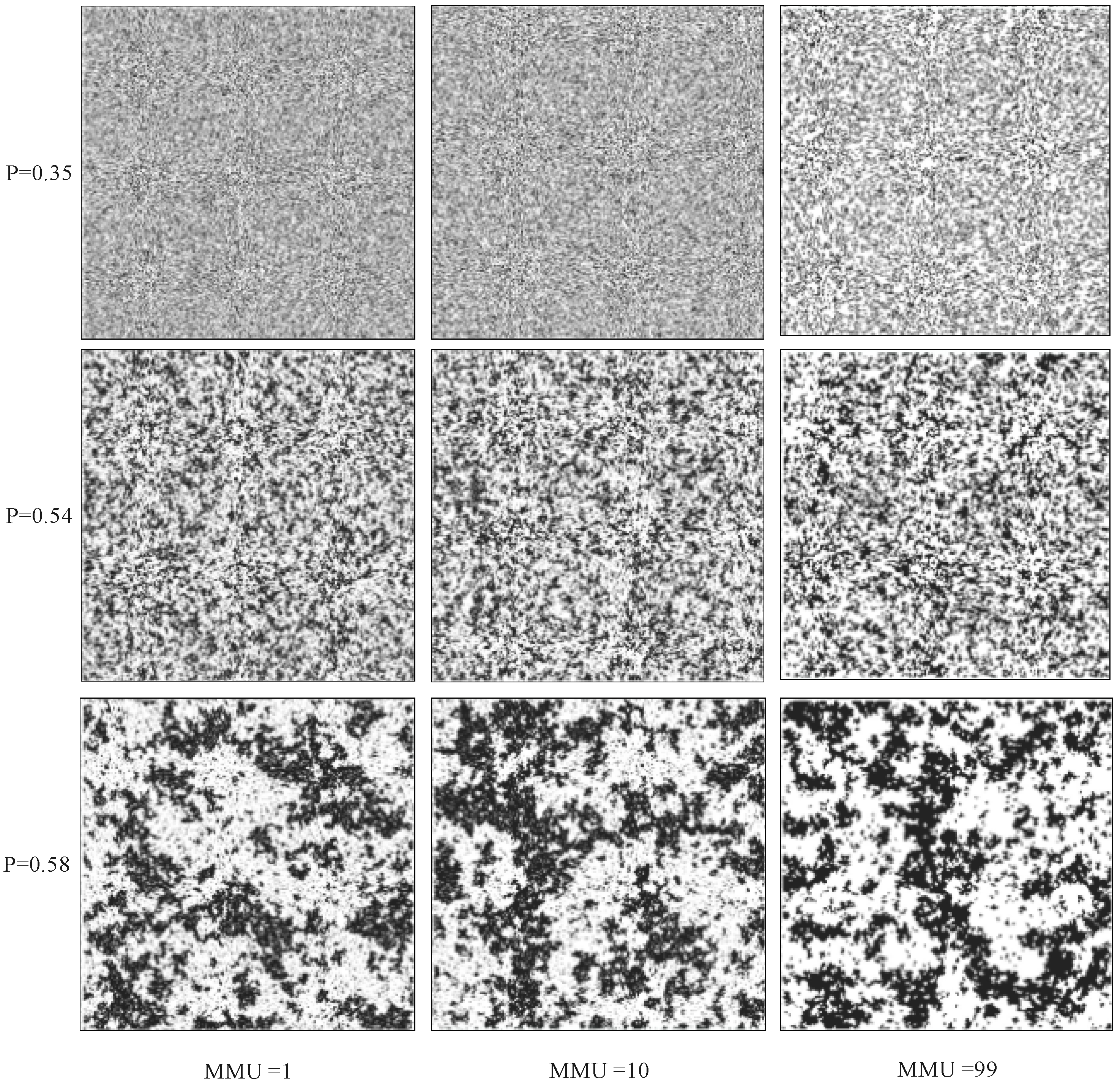
In this paper, therefore, the spatial characteristics of land cover and spatial resolution were simulated to test the sensitivity of thematic errors caused by the positional errors on soft classification accuracy assessment. The purpose of this study was to: (1) examine the impact of positional accuracy on the measures derived from the soft error matrix; (2) provide insight into how this effect changes with varied landscape structure and spatial resolution; and (3) facilitate the consideration of registration for future soft classification accuracy assessment.

2. Methods

2.1. Data Simulation

This paper explores the impact of the positional error on the soft classification using simulated soft maps. Many factors, such as interpreters’ skills, sampling errors and positional errors may simultaneously affect the accuracy assessment of the soft classification using real images. Therefore, using real images makes it nearly impossible to systematically analyze the effect of misregistration. The use of controlled, simulated maps could facilitate the study of thematic errors caused only by positional error without considering the thematic errors caused by other factors. Furthermore, a simulated map is independent of labor-intensive and time-consuming fieldwork necessary to create the classified map and assess the map accuracy. Simulating soft maps can be problematic; we thus followed the strategy developed by [30] in which the soft classification map and its reference map are generated by transforming the initially simulated hard categorical map using a scaling method. The generation of soft maps and modeling positional errors are detailed in following steps.

2.1.1. Simulate Hard Categorical Map with Different Spatial Characteristics

A series of hard categorical maps representing various landscape characteristics were simulated in this study using the SIMMAP software. This software uses the Modified Random Clusters (MRC) method to simulate landscapes whose spatial characteristics are similar to those widely found in real landscapes [31]. SIMMAP has been widely applied for creating controlled, artificial landscapes to study landscape patterns [32,33,34]. Therefore, these simulated maps were used here in place of real landscapes in order to control the factors influencing registration error. The spatial characteristics of various artificial landscapes were controlled using five main parameters: number (NUM) and abundance (A) of the classes, initial probability (P), linear dimension of the pattern (L), minimum mapping unit (MMU) and neighborhood criteria (NC) [31]. Most of these parameters are easily understandable from their names. Initial probability (P) denotes the degree of fragmentation of landscape pattern, and the neighborhood criterion (NC) is the pattern with anisotropy that patches can be placed in a certain dominant direction. The smaller the initial probability, the more fragmented the landscape pattern. The simulated maps will be in a simple random pattern when P is equal to 0, an aggregated pattern with larger patches when P increases, and a single patch filling the entire pattern when P exceeds 0.59 [31]. The MMU adjusts the size of the smallest patch in the simulated map, ranging from 1 (single pixel) to its maximum value 99. Each pixel on the hard categorical map was assigned to a single value ranging from 1 to NUM, representing the class legend (i.e., number of land cover classes). We defined the spatial resolution of the hard pixel as one unit-pixel and the length of pixel as one unit distance in this paper because there is no definition of spatial resolution for a map simulated in SIMMAP.

We simulated three groups of hard categorical maps representing various landscapes with MMU equal to 1, 10 and 99 respectively within which P varied from 0.35 to 0.58 resulting in 24 different maps The spatial characteristics of the simulated maps are listed in Table 1 and are characterized by the following indices: number of patches (NP), mean patch size (MPS), edge length (EL) and mean shape index (MSI). NP and MPS are expressed in pixels and EL is expressed in unit pixel-distance. MSI denotes the irregularity or elongation of the shapes in the pattern with minimum value of 1 and the higher values indicating more convoluted and elongated shapes. The calculation of these indices can be found in the SIMMAP manual [35]. Generally, with higher MMU and P, the NP and EL decreases while the MPS and MSI increases. The MPS is lower in the first group of eight maps, medium in the second group of eight maps, and large in the third group of eight maps. Within each group of eight maps, the fragmentation level changes the NP, EL, MPS and MSI. To simplify the analysis, only two land cover classes (NUM = 2) were considered. The dimensions of each map were 2000 lines by 2000 columns and the abundances of each map class were 60% and 40%, respectively. The simulated landscapes for P equal to 0.35, 0.54 and 0.58 and MMU equal 1, 10 and 99 are presented in Figure 1. These maps are representative of a variety of landscape conditions found on typical land cover maps.

Figure 1. Selectively simulated landscapes (thematic maps) with P being 0.35, 0.54 and 0.58 respectively and MMU being 1, 10 and 99 respectively.

Figure 1. Selectively simulated landscapes (thematic maps) with P being 0.35, 0.54 and 0.58 respectively and MMU being 1, 10 and 99 respectively.

Table 1. The spatial characteristics of the simulated hard categorical maps and the percent of mixed pixels after aggregation using different scales.

MMU	P	NP	MPS	EL	MSI	Percent of Mixed Pixels (%)
						1 × 1	2 × 2	5 × 5	10 × 10
1	0.35	51,443	77.76	1.46 × 106	1.33	0	35.83	92.27	99.98
	0.40	43,502	91.95	1.30 × 106	1.32	0	32.27	88.88	99.91
	0.45	36,796	108.18	1.13 × 106	1.29	0	28.30	83.36	99.60
	0.50	31,887	125.44	938,707	1.24	0	23.31	74.31	98.17
	0.52	30,088	132.09	846,490	1.21	0	21.17	69.45	96.97
	0.54	28,996	137.95	751,605	1.19	0	18.81	63.39	94.79
	0.56	28,433	140.63	647,467	1.16	0	15.91	55.71	90.24
	0.58	28,599	140.06	532,019	1.14	0	13.06	47.32	84.47
10	0.35	17,096	233.97	1.23 × 106	1.82	0	30.52	83.95	99.25
	0.40	14,269	280.33	1.11 × 106	1.78	0	27.73	80.07	98.59
	0.45	11,493	348.04	970,860	1.74	0	24.11	73.70	97.00
	0.50	8479	457.20	789,203	1.67	0	19.73	63.68	92.52
	0.52	7918	505.18	707,103	1.62	0	17.54	57.78	88.62
	0.54	6896	580.05	606,529	1.56	0	15.23	51.35	83.13
	0.56	6496	615.76	506,530	1.50	0	12.71	43.55	74.84
	0.58	6205	644.76	383,276	1.44	0	9.60	33.41	61.54
99	0.35	3567	1121.39	780,243	2.89	0	19.51	57.91	81.74
	0.40	3204	1234.57	756,050	2.81	0	18.81	57.57	82.51
	0.45	2605	2145.92	710,176	2.75	0	17.45	55.73	82.50
	0.50	1864	2312.14	594,092	2.64	0	14.89	49.44	77.98
	0.52	1602	2496.88	530,233	2.58	0	13.23	44.93	73.61
	0.54	1198	3338.90	456,393	2.50	0	11.51	39.57	67.50
	0.56	1030	3883.50	358,173	2.34	0	8.71	30.60	54.08
	0.58	749	5340.45	241,095	2.08	0	5.94	21.09	39.07

Table 1. The spatial characteristics of the simulated hard categorical maps and the percent of mixed pixels after aggregation using different scales.

MMU	P	NP	MPS	EL	MSI	Percent of Mixed Pixels (%)
						1 × 1	2 × 2	5 × 5	10 × 10
1	0.35	51,443	77.76	1.46 × 106	1.33	0	35.83	92.27	99.98
	0.40	43,502	91.95	1.30 × 106	1.32	0	32.27	88.88	99.91
	0.45	36,796	108.18	1.13 × 106	1.29	0	28.30	83.36	99.60
	0.50	31,887	125.44	938,707	1.24	0	23.31	74.31	98.17
	0.52	30,088	132.09	846,490	1.21	0	21.17	69.45	96.97
	0.54	28,996	137.95	751,605	1.19	0	18.81	63.39	94.79
	0.56	28,433	140.63	647,467	1.16	0	15.91	55.71	90.24
	0.58	28,599	140.06	532,019	1.14	0	13.06	47.32	84.47
10	0.35	17,096	233.97	1.23 × 106	1.82	0	30.52	83.95	99.25
	0.40	14,269	280.33	1.11 × 106	1.78	0	27.73	80.07	98.59
	0.45	11,493	348.04	970,860	1.74	0	24.11	73.70	97.00
	0.50	8479	457.20	789,203	1.67	0	19.73	63.68	92.52
	0.52	7918	505.18	707,103	1.62	0	17.54	57.78	88.62
	0.54	6896	580.05	606,529	1.56	0	15.23	51.35	83.13
	0.56	6496	615.76	506,530	1.50	0	12.71	43.55	74.84
	0.58	6205	644.76	383,276	1.44	0	9.60	33.41	61.54
99	0.35	3567	1121.39	780,243	2.89	0	19.51	57.91	81.74
	0.40	3204	1234.57	756,050	2.81	0	18.81	57.57	82.51
	0.45	2605	2145.92	710,176	2.75	0	17.45	55.73	82.50
	0.50	1864	2312.14	594,092	2.64	0	14.89	49.44	77.98
	0.52	1602	2496.88	530,233	2.58	0	13.23	44.93	73.61
	0.54	1198	3338.90	456,393	2.50	0	11.51	39.57	67.50
	0.56	1030	3883.50	358,173	2.34	0	8.71	30.60	54.08
	0.58	749	5340.45	241,095	2.08	0	5.94	21.09	39.07

2.1.2. Generate Soft Classification Map by Aggregation

For hard classification accuracy assessment, whether the impact of positional error is severe or not can depend on the heterogeneity of landscape. Fragmented landscapes increase class boundaries. Pixels located near or at the map class boundary could create thematic errors due to the positional error while the pixels inside the patch would be insensitive to the positional errors [11]. In contrast, for soft classification accuracy assessment, the impact of positional errors not only depends on the heterogeneity of landscape but also may depend on the spatial resolution, which determines the heterogeneity within the pixel. Images/pixels with lower spatial resolution have more mixed pixels and accordingly even slight location errors could largely change the proportion of each class on the reference map. In this paper, the soft classification map was generated by scaling up the hard categorical maps generated using SIMMAP. We aggregated each cluster of pixels on the hard categorical map into a new soft pixel containing a vector denoting the proportion of each class (Figure 2). We varied the cluster size as 1 × 1, 2 × 2, 5 × 5, and 10 × 10 pixels respectively to model different spatial resolutions of the soft map. Accordingly, the spatial resolution of the generated soft maps is 1, 2, 5 and 10 unit distances, respectively, representing from higher resolution to lower resolution. The 1 × 1 cluster size would make all the soft pixels pure since this is the same resolution of the original hard map. Although this situation does not exist in reality, we still included it here for comparison. The 10 × 10 cluster size would make almost all the soft pixels mixed. The percentage of mixed pixels in the soft maps using different scales for all simulated hard categorical maps is presented in Table 1. The greater the fragmentation and the smaller the mean patch size of the landscape, the higher will be the percentage of the mixed pixels. We regarded these aggregated maps as the soft classification maps. If we compared these soft classification maps with the hard categorical maps using a soft classification matrix [7], their thematic accuracy would be one hundred percent.

Figure 2. Example of a simulated soft classification and reference pixel (spatial resolution: 5 unit distance) at levels of 0.0, 0.1, 0.2 and 0.3 soft pixel’s positional error respectively in in both x and y direction. The proportion of two classes was greatly changed due to the different levels of positional errors.

Figure 2. Example of a simulated soft classification and reference pixel (spatial resolution: 5 unit distance) at levels of 0.0, 0.1, 0.2 and 0.3 soft pixel’s positional error respectively in in both x and y direction. The proportion of two classes was greatly changed due to the different levels of positional errors.

2.1.3. Simulating Positional Errors

Once the soft classification maps were created, it was necessary to simulate positional errors to evaluate their impact on the thematic accuracy of the map. Positional errors typically vary spatially over the map [12]. In this study, we simulated the positional errors using a uniform model as it is very complicated to model these positional errors practically. The uniform model assumed that the positional errors were equally distributed between the classification map and the reference map and were modeled by translation using the methods developed by [16,17] in research on quantifying the effect of misregistration in change detection analysis. Therefore, for a soft pixel at location (x, y) on the soft classification map generated as previously described, we used the cluster at location (x + i, y + i) on the hard categorical map as the reference unit, where i is the number of soft pixels off its original position and i varied from 0 to 3 soft pixels with an addition of 0.1 soft pixels. After translation, the reference unit is $\sqrt{2}i$ from the corresponding soft pixel. This factor is used because registration accuracy is commonly reported as “the registration accuracy between the classification map and reference map is within a half of a pixel.” However, it is important to note that a half pixel for different spatial resolutions implies a different absolute distance. For example, a half of a pixel of Landsat TM 5 is 15 m while half of a pixel of MODIS imagery is 500 m. In this paper, a half-soft pixel’s misregistration in a soft map with a spatial resolution of 10 unit distance means 5 unit distance, while for a soft map with a spatial resolution of 5 unit distance means 2.5 unit distance. Sub-pixel misregistration is performed as shown in Figure 2. We apply this translation model to every soft classification pixel on the soft maps (except the soft pixels located at the four borders of the map), then record the proportion of change for every soft pixel by shift in order to create the soft reference map with positional errors. Figure 2 shows an example of the generation of the soft classification pixel and its reference pixel with positional errors of 0.1, 0.2 and 0.3 soft pixels.

2.2. Accuracy Assessment

Once the soft classification and reference maps were generated and the maps were subjected to registration error, an assessment could then be conducted to evaluate the errors. In this study, the composite operator developed by [7] was used for constructing the soft classification matrix (SCM) because of its three practical and reasonable characteristics: sum of entries being 1, diagonal matrix for identical maps, and constant marginal totals. The composite operator consists of different calculations for the diagonal and off-diagonal elements (Equation (1)). The diagonal elements (where i equals j) employ the minimum operator, the ruling principle of which is that the agreement of elements cannot exceed the minimum value of two proportions. The off-diagonal elements employ the mathematical formula in Equation (1) when i ≠ j. The core idea of this formula is that the proportion of class i incorrectly classified as class j, denoted as p_nij, is computed by distributing the commission proportion of class i $c_{ni}-p_{nii}$ according to the ratio of omission proportion of class j $c_{ni}-p_{nii}$ to the total omission proportion of all classes ${\displaystyle {\sum }_{j=1}^k(r_{nj}-p_{njj})}$ [7]. Table 2 shows the sub-pixel error matrix constructed for the nth soft pixel. The sum of each row and column is equal to the proportion of each class classified and the true proportion of reference data, respectively. The sum of the diagonal and off-diagonal elements is equal to one unit in the SCM for each sampled pixel. The SCM was first constructed for each soft pixel and then the final SCM was created by averaging the SCMs for all pixels between the soft classification map and corresponding reference map (Table 3). From the SCM, we derived overall accuracy and kappa which are the most commonly used accuracy measures at the map level in remote sensing.

$$p_{nij}=\{\begin{array}{r}MIN(c_{ni},r_{nj}),i=j\\ (c_{ni}-p_{nii})\times \left[(r_{nj}-p_{njj})/{\displaystyle \sum _{j=1}^k(r_{nj}-p_{njj})}\right],i\ne j\end{array}$$

(1)

Overall accuracy and kappa will fluctuate given the varied positional errors introduced in the classification map and reference data. When the soft classification map and reference data are perfectly registered, the overall accuracy and kappa represent the actual thematic accuracy. However, in this study, we are particularly interested in the component of the thematic error that is introduced by the positional errors only. This part of the thematic error equals the accuracy resulting from the soft error matrix without positional errors minus its counterpart with positional errors. In this paper, the thematic error for overall accuracy is denoted as the OA-error and for kappa the kappa-error. In this study, the overall accuracy is 100% and kappa is 1 when there is no positional error because the reference data were created from the land cover maps and there is no error.

Table 2. Sub-pixel error matrix for the nth pixel.

Classification	Reference				Total
	Class 1	Class 2	…	Class k
Class 1	pn11	pn12	…	pn1k	cn1
Class 2	pn21	pn22	…	pn2k	cn2
…	…	…	…	…	…
Class k	pnk1	pnk2	…	pnkk	cn3
Total	rn1	rn2	…	rnk

Table 2. Sub-pixel error matrix for the nth pixel.

Classification	Reference				Total
	Class 1	Class 2	…	Class k
Class 1	pn11	pn12	…	pn1k	cn1
Class 2	pn21	pn22	…	pn2k	cn2
…	…	…	…	…	…
Class k	pnk1	pnk2	…	pnkk	cn3
Total	rn1	rn2	…	rnk

Table 3. Error matrix for soft classification.

Classification	Reference				Total
	Class 1	Class 2	…	Class k
Class 1	P11	P12	…	P1k	P1+
Class 2	P21	P22	…	P2k	P2+
…	…	…	…	…	…
Class k	Pk1	Pk2	…	Pkk	Pk+
Total	P+1	P+2	…	P+k
Accuracy measures	$Oa=\frac{\sum P_{ii}}{n}\times 100\%, Kappa=\frac{n{\sum }_{\mathrm{i}}^{\mathrm{k}}{\mathrm{P}}_{ii}-{\sum }_{\mathrm{i}}^{\mathrm{k}}{\mathrm{P}}_{\mathrm{i}+}{\mathrm{P}}_{+\mathrm{i}}}{n^2-{\sum }_{\mathrm{i}}^{\mathrm{k}}{\mathrm{P}}_{\mathrm{i}+}{\mathrm{P}}_{+\mathrm{i}}}$
	$Ua=\frac{P_{ii}}{P_{i+}} Pa=\frac{P_{jj}}{P_{+j}}$

Table 3. Error matrix for soft classification.

Classification	Reference				Total
	Class 1	Class 2	…	Class k
Class 1	P11	P12	…	P1k	P1+
Class 2	P21	P22	…	P2k	P2+
…	…	…	…	…	…
Class k	Pk1	Pk2	…	Pkk	Pk+
Total	P+1	P+2	…	P+k
Accuracy measures	$Oa=\frac{\sum P_{ii}}{n}\times 100\%, Kappa=\frac{n{\sum }_{\mathrm{i}}^{\mathrm{k}}{\mathrm{P}}_{ii}-{\sum }_{\mathrm{i}}^{\mathrm{k}}{\mathrm{P}}_{\mathrm{i}+}{\mathrm{P}}_{+\mathrm{i}}}{n^2-{\sum }_{\mathrm{i}}^{\mathrm{k}}{\mathrm{P}}_{\mathrm{i}+}{\mathrm{P}}_{+\mathrm{i}}}$
	$Ua=\frac{P_{ii}}{P_{i+}} Pa=\frac{P_{jj}}{P_{+j}}$

3. Results

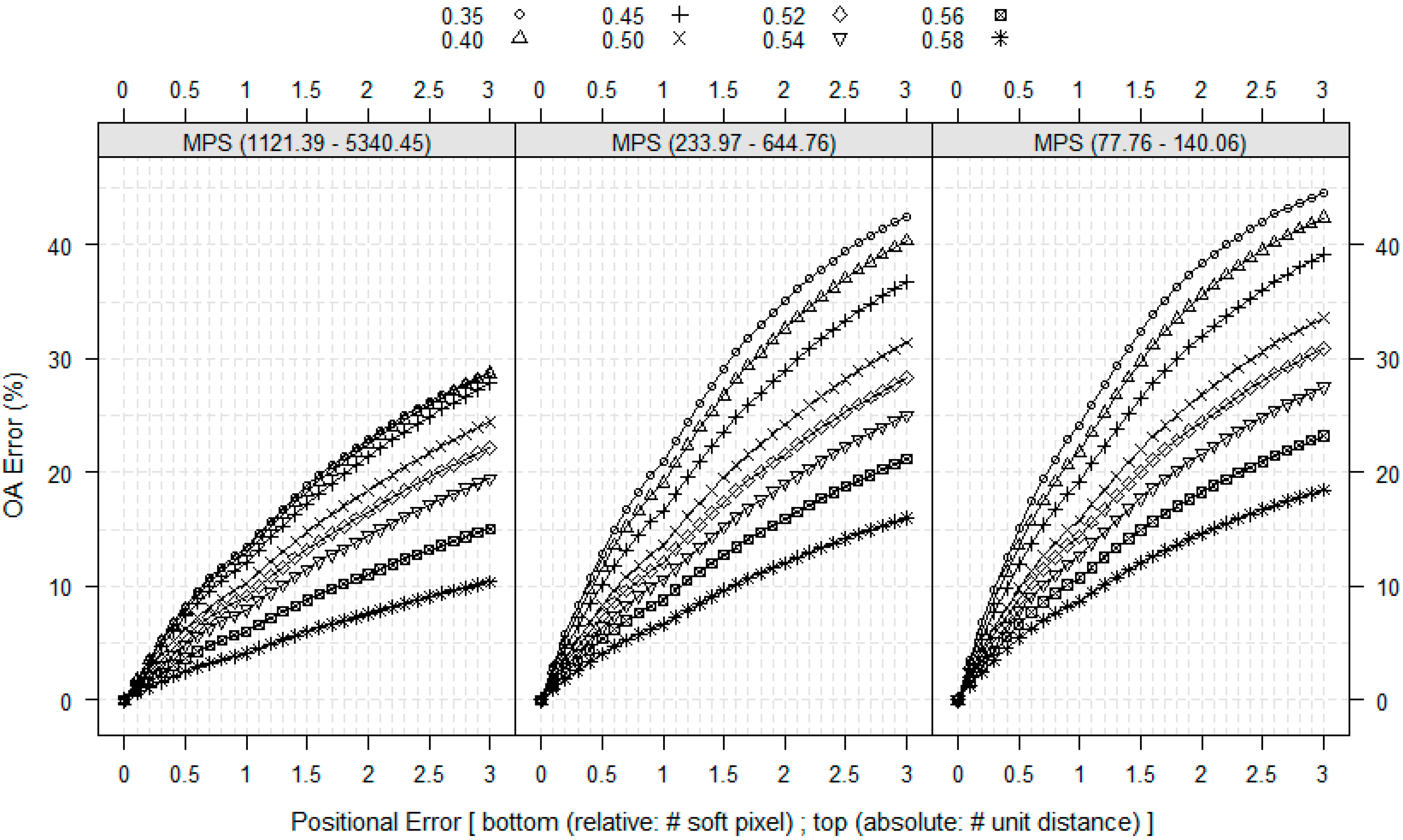
Figure 3, Figure 4, Figure 5 and Figure 6 show the relationship between OA-errors and the positional errors while Figure 7, Figure 8, Figure 9 and Figure 10 show the link between kappa-errors and the positional errors where the spatial resolution is 1, 2, 5, and 10 unit distances, respectively. Each figure presents the relationship divided into three groups by MPS: large MPS or mean patch size (1121.39–5340.05), middle MPS (233.97–644.76, and small MPS (77.76–140.06) from the left to the right. Within each group, the P value (representing the fragmentation) varies from 0.35 to 0.58 and the MPS also varies accordingly. The bottom abscissa value is the relative distance based on the soft pixel associated with a given spatial resolution while the top abscissa value is the absolute distance based on the unit distance corresponding to the relative distance. The same relative positional error appears to have different absolute distance because of the spatial resolution.

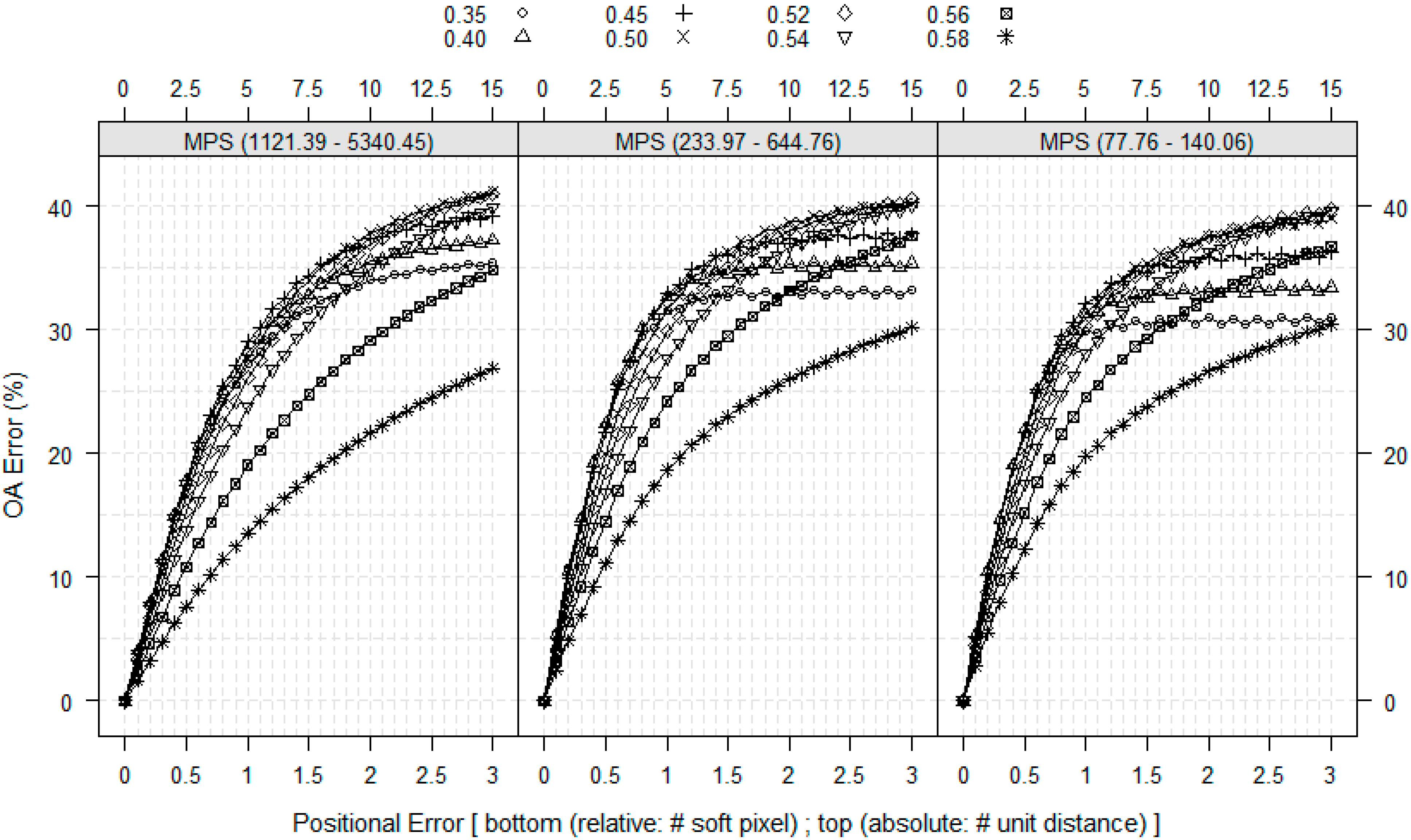
Figure 3 reveals the impact of a positional error ranging from 0 to 3 pixels on the OA-error with varying fragmentation and MPS at a spatial resolution of 1 unit distance. It was determined that as a positional error increases, so do the OA-errors. When there was no positional error, there was no OA-error. The rate of growth is different depending on the amount of fragmentation and MPS. For example, the rate is very high when the P is 0.35 and MPS is 77.76, whereas the rate is low when P is 0.58 and MPS is 5340.45. Generally, smaller MPS and higher fragmentation (lower P values) produced a greater positional error effect on OA-error. As can be seen in Figure 3, the corresponding lines in the left group (MPS of larger size) are lower than the middle group (MPS of medium size) which is lower than the right group (MPS of small size). At the positional error of three soft pixels, the largest impact results in an OA-error of 44.6% while the least impact produces only 10.4%.

Figure 3. Impact of positional error on OA-error at different landscape characteristics using a spatial resolution of 1 unit distance.

Figure 3. Impact of positional error on OA-error at different landscape characteristics using a spatial resolution of 1 unit distance.

Figure 4. Impact of positional error on OA-error at different landscape characteristics using a spatial resolution of 2 unit distance.

Figure 4. Impact of positional error on OA-error at different landscape characteristics using a spatial resolution of 2 unit distance.

Figure 5. Impact of positional error on OA-error at different landscape characteristics using a spatial resolution of 5 unit distance.

Figure 5. Impact of positional error on OA-error at different landscape characteristics using a spatial resolution of 5 unit distance.

Figure 6. Impact of positional error on OA-error at different landscape characteristics using a spatial resolution of 10 unit distance.

Figure 6. Impact of positional error on OA-error at different landscape characteristics using a spatial resolution of 10 unit distance.

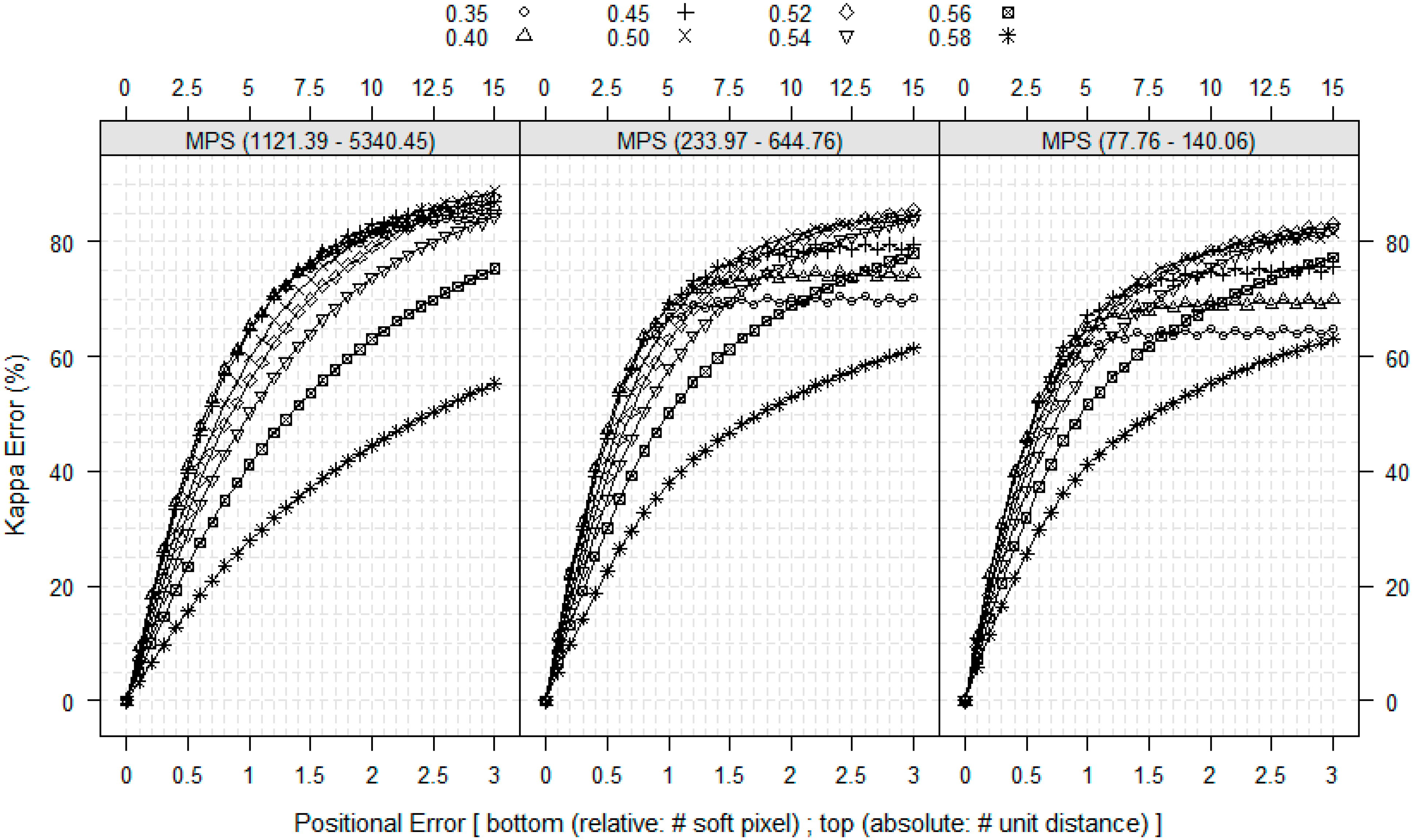
Figure 7. Impact of positional error on kappa-error at different landscape characteristics using a spatial resolution of 1 unit distance.

Figure 7. Impact of positional error on kappa-error at different landscape characteristics using a spatial resolution of 1 unit distance.

Figure 8. Impact of positional error on kappa-error at different landscape characteristics using a spatial resolution of 2 unit distance.

Figure 8. Impact of positional error on kappa-error at different landscape characteristics using a spatial resolution of 2 unit distance.

Figure 9. Impact of positional error on kappa-error at different landscape characteristics using a spatial resolution of 5 unit distance.

Figure 9. Impact of positional error on kappa-error at different landscape characteristics using a spatial resolution of 5 unit distance.

Figure 10. Impact of positional error on kappa-error at different landscape characteristics using a spatial resolution of 10 unit distance.

Figure 10. Impact of positional error on kappa-error at different landscape characteristics using a spatial resolution of 10 unit distance.

The results of Figure 3 also hold in Figure 4 where the spatial resolution is 2 unit distance. The only difference is that the 2 unit distance spatial resolution creates less impact of positional error on the OA-error than the 1 unit distance with the same amount of absolute distance but creates greater impact with the same amount of relative distance. For instance, the 3 unit distance positional error created nearly 28.8% OA-error when P equals 0.35 with MPS being 1121.39 at the spatial resolution of 1 unit distance, whereas its counterpart created 27.2% OA-error at the spatial resolution of 2 unit distance. However, the 3 soft pixel positional error created nearly 28.8% OA-error when P equals 0.35 with MPS being 1121.39 at the spatial resolution of 1 unit distance, whereas its counterpart creates 35.5% OA-error at the spatial resolution of 2 unit distance. It was also found that some of the lines with P being 0.35 and 0.40 show a trend of becoming stable in the middle and small MPS groups when positional errors are greater than 1.5 soft pixels.

These results change when the spatial resolution is increased to 5 unit distance (Figure 5). Compared with Figure 3 and Figure 4, the lowest impact remained the same while the highest impact is not when P equals to 0.35 but when P is equal to 0.45 or 0.50. The lines at P equals 0.35, 0.40 and 0.45 show a trend becoming stable after the positional errors reach 1 soft pixel. Compared to what was shown in Figure 3 and Figure 4, the corresponding lines with the same fragmentation lie in different groups of MPS and do not have much difference.

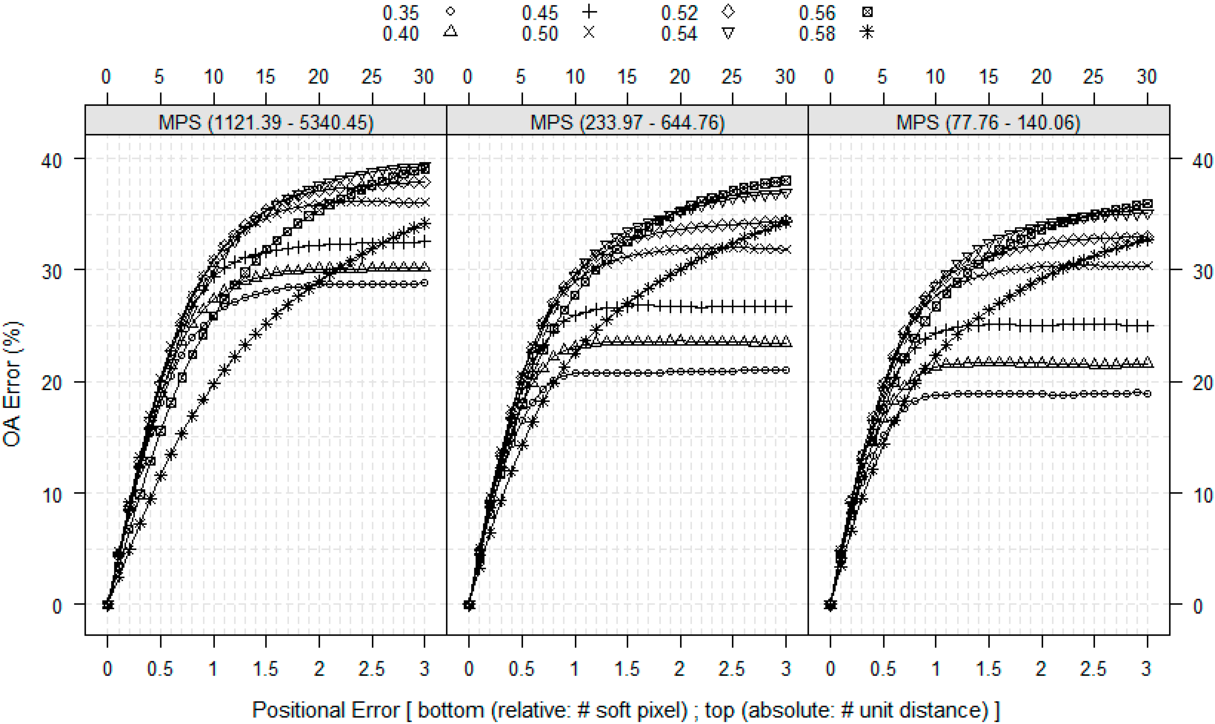
Compared to the spatial resolutions of 1, 2, and 5 unit distances, the pattern at a spatial resolution of 10 unit distance are clearly different (Figure 6). The highest impact is shown on the line with P being 0.54 or 0.56 for all groupings of MPS. However, the lowest impact is shown on the line with P being 0.58 when the positional error is small, but changes to P being 0.35 when the positional error is large. The corresponding lines in the left group (MPS of larger size) are higher than the middle group (MPS of medium size) which is higher than the right group (MPS of small size), which is the complete opposite of the results from Figure 3 and Figure 4.

A comparison of Figure 3 to Figure 6 by MPS grouping shows that under the same spatial characteristics, the spatial resolution alters the impact of positional error on the OA-error. For example, with P being 0.58 and MPS being 5340.45, the OA-error ranges from 0% to 10.4% at the spatial resolution of 1 unit distance while it varies from 0% to 34.2% at the spatial resolution of 10 unit distance. As the spatial resolution becomes coarser, the group of lines becomes denser, meaning that the degree of influence of fragmentation is less. It also shows as the spatial resolution becomes coarser, the three groups of MPS do not change the shape of the lines as much with the same fragmentation.

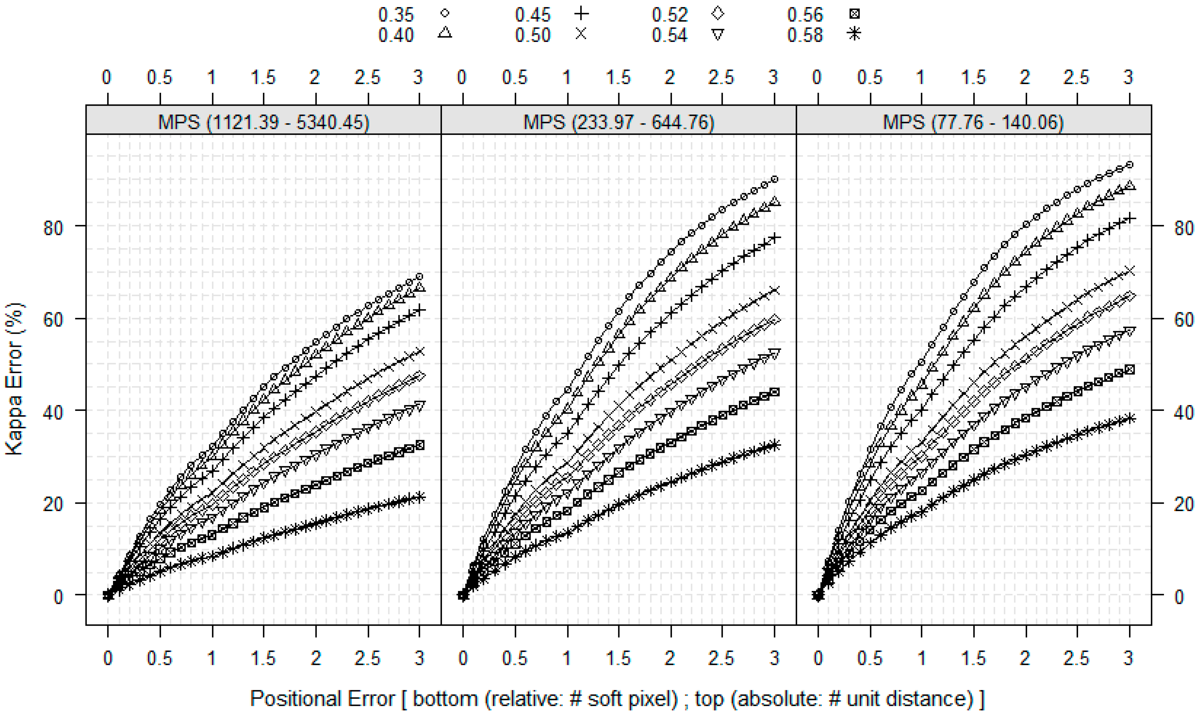
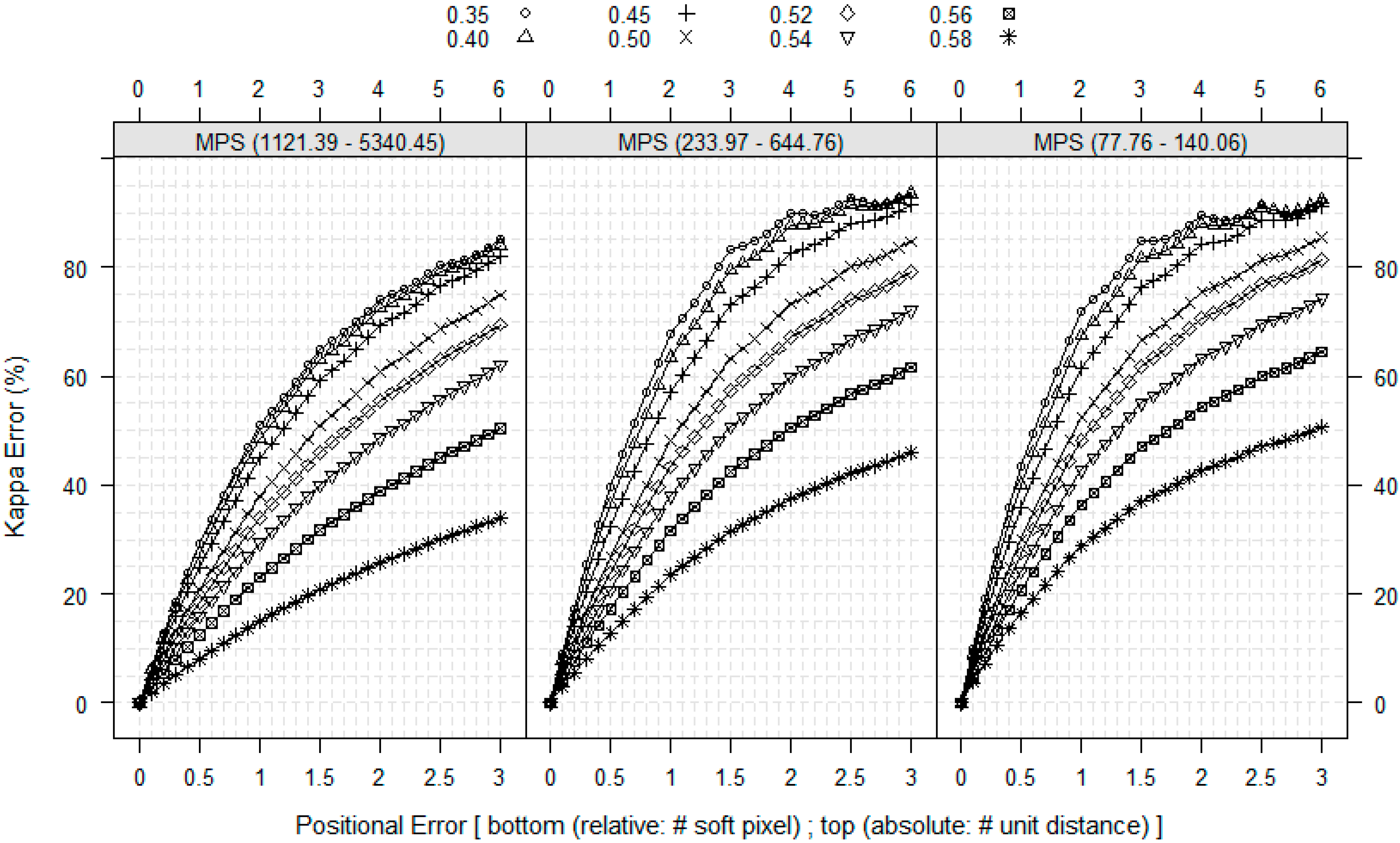
The same analysis that was performed with OA-error can also be shown using kappa-error. Compared to the impact of positional error on the OA-error, the effect on the kappa-error is higher (Figure 7, Figure 8, Figure 9 and Figure 10). With three soft pixel positional errors, the kappa-error ranges from 0% to 93.7%. The patterns of fragmentation and MPS are the same as was found in OA-error analysis.

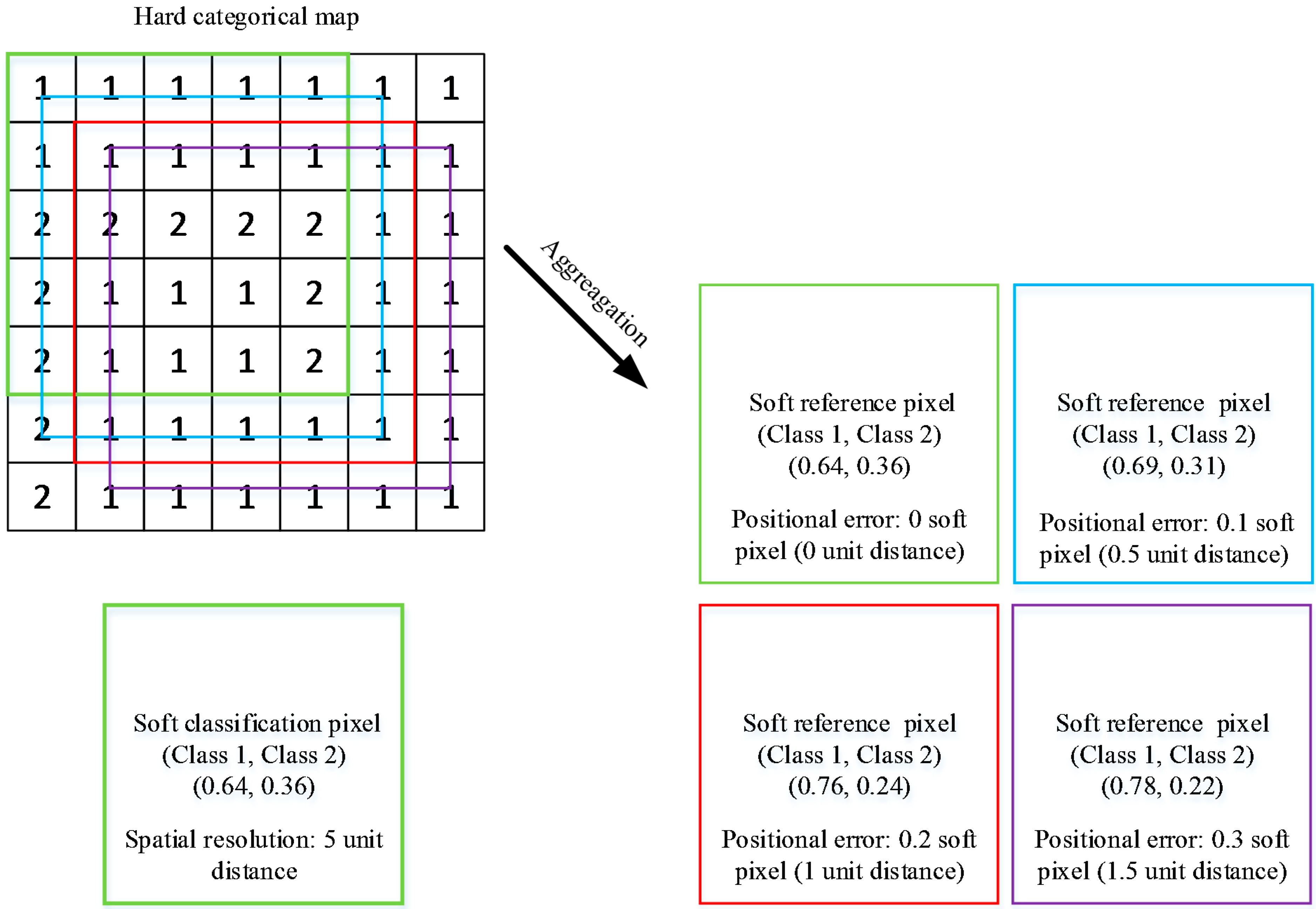
Table 4 shows the required registration accuracy (# of soft pixels) to keep the OA and kappa error under 10% for different landscape patterns at a spatial resolution of 1, 2, 5, and 10 unit distance respectively. A value of 10% was selected here as a reasonable amount of error contribution from positional error in a typical thematic accuracy assessment. It is clear that for most landscape patterns simulated here, a half of a soft-pixel registration accuracy is not sufficient to guarantee the OA-error is less than 10% except when the spatial resolution is 1 unit distance. To retain the OA-error at less than 10%, the required registration accuracy for a spatial resolution of 1 unit distance ranges from 0.3 to 2.8 soft pixels with an average of 0.85 pixels. This requirement then translates to a range of from 0.2 to 1.4 soft pixels, 0.1 to 0.6 soft pixels, and 0.2 to 0.4 soft pixels at spatial resolutions of 2, 5, and 10 unit distances, respectively. To retain the kappa-error at less than 10%, the required registration accuracy for spatial resolution of 1, 2, 5, and 10 unit distances range from 0.1 to 1.1 soft pixels, 0.1 to 0.6 soft pixels, 0.1 to 0.3 soft pixels and less than 0.1 to 0.1soft pixels, respectively. As the spatial resolution gets coarser, the required average positional accuracy varied from 0.86 to 0.22 for overall accuracy and from 0.29 to less than 0.1 for kappa.

Table 4. The required registration accuracy (# soft pixels) to keep the OA- and kappa-errors under 10% for different landscape characteristics at the spatial resolution of 1, 2, 5, 10 unit distances respectively. (“<” represents “less than”).

P	MPS	Less than 10% OA-Error				Less than 10% Kappa-Error
		1	2	5	10	1	2	5	10
0.35	77.76	0.3	0.2	0.1	0.2	0.1	0.1	0.1	0.1
0.40	91.95	0.3	0.2	0.1	0.2	0.1	0.1	<0.1	0.1
0.45	108.18	0.4	0.2	0.1	0.2	0.1	0.1	<0.1	<0.1
0.50	125.44	0.5	0.3	0.2	0.2	0.2	0.1	0.1	<0.1
0.52	132.09	0.5	0.3	0.2	0.2	0.2	0.1	0.1	<0.1
0.54	137.95	0.6	0.4	0.2	0.2	0.2	0.1	0.1	0.1
0.56	140.63	0.8	0.5	0.3	0.2	0.3	0.2	0.1	0.1
0.58	140.06	1.1	0.6	0.3	0.3	0.4	0.2	0.1	0.1
0.35	233.97	0.3	0.2	0.1	0.2	0.1	0.1	<0.1	0.1
0.40	280.33	0.4	0.2	0.1	0.2	0.1	0.1	<0.1	0.1
0.45	348.04	0.4	0.3	0.2	0.2	0.1	0.1	<0.1	<0.1
0.50	457.20	0.6	0.3	0.2	0.2	0.2	0.1	0.1	<0.1
0.52	505.18	0.7	0.4	0.2	0.2	0.2	0.1	0.1	<0.1
0.54	580.05	0.9	0.5	0.2	0.2	0.3	0.2	0.1	0.1
0.56	615.76	1.1	0.6	0.3	0.2	0.4	0.2	0.1	0.1
0.58	644.76	1.5	0.8	0.4	0.3	0.6	0.3	0.2	0.1
0.35	1121.39	0.6	0.3	0.2	0.2	0.2	0.1	0.1	<0.1
0.40	1234.57	0.6	0.4	0.2	0.2	0.2	0.1	0.1	<0.1
0.45	2145.92	0.7	0.4	0.2	0.2	0.2	0.1	0.1	<0.1
0.50	2312.14	0.9	0.5	0.2	0.2	0.3	0.2	0.1	<0.1
0.52	2496.88	1.0	0.5	0.3	0.2	0.4	0.2	0.1	<0.1
0.54	3338.90	1.2	0.6	0.3	0.2	0.4	0.2	0.1	<0.1
0.56	3883.50	1.7	0.9	0.4	0.3	0.6	0.3	0.1	0.1
0.58	5340.45	2.8	1.4	0.6	0.4	1.1	0.6	0.3	0.1
Average		0.85	0.46	0.23	0.22	0.29	0.17	0.12	<0.1

Table 4. The required registration accuracy (# soft pixels) to keep the OA- and kappa-errors under 10% for different landscape characteristics at the spatial resolution of 1, 2, 5, 10 unit distances respectively. (“<” represents “less than”).

P	MPS	Less than 10% OA-Error				Less than 10% Kappa-Error
		1	2	5	10	1	2	5	10
0.35	77.76	0.3	0.2	0.1	0.2	0.1	0.1	0.1	0.1
0.40	91.95	0.3	0.2	0.1	0.2	0.1	0.1	<0.1	0.1
0.45	108.18	0.4	0.2	0.1	0.2	0.1	0.1	<0.1	<0.1
0.50	125.44	0.5	0.3	0.2	0.2	0.2	0.1	0.1	<0.1
0.52	132.09	0.5	0.3	0.2	0.2	0.2	0.1	0.1	<0.1
0.54	137.95	0.6	0.4	0.2	0.2	0.2	0.1	0.1	0.1
0.56	140.63	0.8	0.5	0.3	0.2	0.3	0.2	0.1	0.1
0.58	140.06	1.1	0.6	0.3	0.3	0.4	0.2	0.1	0.1
0.35	233.97	0.3	0.2	0.1	0.2	0.1	0.1	<0.1	0.1
0.40	280.33	0.4	0.2	0.1	0.2	0.1	0.1	<0.1	0.1
0.45	348.04	0.4	0.3	0.2	0.2	0.1	0.1	<0.1	<0.1
0.50	457.20	0.6	0.3	0.2	0.2	0.2	0.1	0.1	<0.1
0.52	505.18	0.7	0.4	0.2	0.2	0.2	0.1	0.1	<0.1
0.54	580.05	0.9	0.5	0.2	0.2	0.3	0.2	0.1	0.1
0.56	615.76	1.1	0.6	0.3	0.2	0.4	0.2	0.1	0.1
0.58	644.76	1.5	0.8	0.4	0.3	0.6	0.3	0.2	0.1
0.35	1121.39	0.6	0.3	0.2	0.2	0.2	0.1	0.1	<0.1
0.40	1234.57	0.6	0.4	0.2	0.2	0.2	0.1	0.1	<0.1
0.45	2145.92	0.7	0.4	0.2	0.2	0.2	0.1	0.1	<0.1
0.50	2312.14	0.9	0.5	0.2	0.2	0.3	0.2	0.1	<0.1
0.52	2496.88	1.0	0.5	0.3	0.2	0.4	0.2	0.1	<0.1
0.54	3338.90	1.2	0.6	0.3	0.2	0.4	0.2	0.1	<0.1
0.56	3883.50	1.7	0.9	0.4	0.3	0.6	0.3	0.1	0.1
0.58	5340.45	2.8	1.4	0.6	0.4	1.1	0.6	0.3	0.1
Average		0.85	0.46	0.23	0.22	0.29	0.17	0.12	<0.1

4. Discussion

Quantifying the accuracy of sub-pixel land cover maps derived from the soft classification of remote sensing images is crucial for the future development of fields such as ecological and environmental modeling which incorporate land cover information as an important variable. The error matrix has been widely applied for accuracy assessment because of its practicality and effectiveness. Recent research has shown that much effort has been made to generalize a soft classification error matrix from the traditional one. The soft error matrix has the same accuracy measures as the traditional one. However, the impact of positional error on the soft classification thematic accuracy is uncertain and has not been addressed explicitly. In this paper, the impact of positional errors on thematic accuracy of soft classification was examined including the effects introduced by landscape structure and spatial resolution. A series of soft classifications with varied landscape patterns and the corresponding reference data were simulated and a sub-pixel misregistration model was implemented. The thematic errors caused by positional errors were reported using overall accuracy and kappa.

Our results showed that the effects of positional error on thematic accuracy as computed from a soft error matrix cannot be ignored. Most previous research in this field on the impact of positional accuracy on thematic accuracy used Landsat Thematic Mapper (TM) imagery and did not examine soft classification. Our work employed artificially generated maps representing various landscape patterns and simulation of soft classifications making our results difficult to directly compare to the previous work. However, there are still some important similarities between our work and this previous work. Patterson and Williams [36] reported that positional error could reach up to one pixel and could be located anywhere in a 3 × 3 pixel grouping [37]. Given this amount of positional error, the results of our simulations showed errors of overall accuracy ranging from 4.12% to 34.3%, whereas the error of kappa ranged from 8.47% to 71.76%. Kappa is more sensitive to the positional error largely because kappa uses the off-diagonal elements of the error matrix in the calculation of the statistic, whereas overall accuracy does not. These results are consistent with [19,38] who indicated that 30% percent of thematic errors were attributed to misregistration for Landsat pixels. Therefore, the results of this research provide further confirmation of previous work.

This paper determined that a half-pixel (as determined for Landsat Thematic Mapper imagery) is not appropriate for all spatial resolutions when performing a soft classification accuracy assessment. In this paper, a half-pixel was found to be sufficient only when the map used was of 1 unit distance spatial resolution. As the spatial resolution becomes coarser, the positional requirement increases. Therefore, the positional accuracy standard for the soft classification accuracy assessment should be updated and the future requirement for registration accuracy must consider the spatial resolution of the imagery. In reality, the half-pixel standard was defined from the application of SPOT and Landsat TM imagery [14,39]. Whether this is suitable for the MODIS and other remotely sensed images with lower spatial resolution also needs to be examined. From our research, we can deduce that the required positional accuracy for MODIS is greater than the half-pixel required for SPOT and Landsat TM.

In the past few years, much effort has been made to develop complicated algorithms for generalizing the conventional error matrix to the soft error matrix [7,8]. However, requirements suitable for the hard classification accuracy may not be suitable for the soft one. We suggest examining the assumptions, procedures, and accuracy measures created for the hard error matrix and applying these for the soft classification accuracy assessment including sampling scheme and explanation of accuracy measures. This research has also provided some insights when considering the sampling location for collecting the reference data for comparison with the map in creating the error matrix. It has shown that the chance of misclassifying a pixel increased in places where the patch size was smaller and heterogeneity was higher [20,40]. The aim of any sampling design for accuracy assessment is to present these thematic errors proportionally in the error matrix and, therefore, a great deal of effort had been made to develop the most efficient sampling schemes to minimize the sampling error [41,42]. However, the existence of positional error introduces false information into the error matrix, thereby causing more error than just the error due to sampling. In addition, the influence of the positional error was also higher where the landscape was more heterogeneous with smaller patch size, especially when the spatial resolution was higher. Therefore, sampling in only the homogeneous areas will result in overestimating the accuracy [43] but sampling that includes the heterogeneous areas risks increasing the false accuracy information. How to design sampling schemes considering positional errors requires further research.

Our research has complemented the efforts to assess the impact of positional error on the thematic accuracy under different spatial resolutions and spatial characteristics of landscape for soft classification. This impact was a function of landscape variables, degree of registration, and spatial resolution. At high spatial resolutions we noted that the more fragmented and the smaller patch sizes of the landscape, the greater the effect of positional error. However, at lower spatial resolutions, the trend noted for higher spatial resolutions changed. This trend reversal for lower spatial resolutions can be explained in that the larger pixel sizes have more chance to shift to a new location, although the proportion of class membership within the pixel remains similar when the landscape is heterogeneous. Therefore, it appears as if the pixel has not moved even though it has.

This research has also provided some implications for soft change detection analysis. If the reference map and classification map in this paper are treated as two maps from different dates, all the results and conclusions are suitable for the change detection using soft classification. These results then complement the work of [16] who examined the requirement of positional accuracy for change detection using hard classification for Landsat TM data and concluded that less than one-fifth of a pixel is required to achieve a change detection error of less than 10%.

A number of limitations also remain. First, this research only employs artificial images to create landscape patterns, and the differences between these simulated images and real satellite images need consideration. Second, this research only took into account two classes with fixed class proportions as dictated by the Modified Random Clusters model for simulation. Simulating more than two classes with different spatial characteristics is difficult to keep the proportion of classes the same. We can speculate that more classes will increase the impact of the positional errors because it increases the fragmentation and decreases the patch size. We can also deduce that one dominating class with other minor classes will decrease the impact because it increases the mean patch size. Finally, this paper ignored the distribution of the positional errors. Positional errors are not equally distributed over the spatial map [12] and the modeling of the distribution of the positional errors will be a task for future research.

5. Conclusions

This paper conducted an analysis of the impact of positional error on thematic accuracy for soft accuracy assessment using simulated maps of various landscape patterns at different spatial resolutions. Some of the results of this work were quite predictable, while others were not, thus having specific implications on the impact of positional error on thematic error when assessing map accuracy. Not surprisingly, increased fragmentation of the landscape increased the impact of positional error on thematic accuracy. Also not surprisingly, initially larger pixels increased the impact of positional error on thematic accuracy as the larger pixels cause increased fragmentation. However, what is surprising is that this trend did not continue as the pixel size increased. Instead, the larger pixels reached a point in which the proportion of map classes within a large, soft pixel reached an equilibrium regardless of the positional error. This result has special significance when considering low spatial resolution imagery such as AVHRR or MODIS data. Another very interesting and practical result of our work showed that a half-pixel is not sufficient to keep the thematic error under 10% for all spatial resolutions for soft classification accuracy assessment. A half-pixel registration error is commonly accepted for moderate resolution imagery such as Landsat Thematic Mapper and SPOT. A 10% error contribution from positional error is a reasonable amount that might be accepted in a thematic map accuracy assessment. However, at various spatial resolutions tested in this study, it was determined that a half-pixel registration error does not keep the thematic error under 10%. Detailed figures were provided to allow the reader to determine the impact of positional error at varying landscape patterns and spatial resolutions. Finally, the impact of positional error on the thematic accuracy changes with variation in landscape variables, degree of registration, and spatial resolution. There is a great need to update the positional requirements for soft accuracy assessment according to the map spatial resolution and landscape structure. In addition, the results and conclusions in this paper are also suitable for soft change detection analysis. Careful consideration of the issues and analysis described in this paper will result in improved soft accuracy assessment in the future.