1. Introduction
Over the last three decades, remote sensing has played an important role in agricultural monitoring and land-cover/land-use classification [
1,
2]. The identification of the crops and their spatial distribution allows farmers and policy makers to make better decisions regarding management practices. At a global and regional scale, mapping extensive crops is carried out effectively through the analysis of remote-sensing images with a spatial resolution of 15 m or greater (e.g., images coming from sensors such as ETM+ or ASTER). Nevertheless, images of this type are not suitable for modeling fragmented agricultural landscapes (with parcels of 5 ha or less), because a precise delimitation of the parcels is required for its analysis; and this resolution does not allow a representation of the spatial behavior of the parcels of intensive cultivation [
3]. In this regard, the use of very-high resolution (VHR, 1m or less) images allows analyzing these complex landscape patterns through the visual identification of different crop parcels. However, this higher resolution represents a challenge for available data exploitation and dissemination approaches.
Digital processing on VHR images represents a restraint for traditional pixel-based approaches, because of two main reasons [
4,
5]: (1) high spectral variability within natural and semi-natural covers produces a low classification accuracy; and (2) a pixel is only a mere consequence of the discrete representation of an image, therefore, it lacks of semantic meaning in the real world and consequently is pointless for end users. These problems have led to a paradigm shift from a pixel-based to an object-based approach [
4,
6,
7]. Object-based image analysis, in a geographic context known as GEOBIA, outperforms VHR image analysis, when compared to pixel-based approach [
8]. For example, [
9,
10,
11,
12] point out that object-based classification produces more homogeneous land cover classes with higher overall accuracy compared to the results of pixel-based classifications. This occurs because GEOBIA methods are more robust to within-class spectral variability than pixel-based algorithms, where the minimal information units (pixels) do not keep a correspondence with the scale of the phenomenon under analysis.
Broadly speaking, the GEOBIA approach starts with a segmentation process, followed by successive analyses, usually at different hierarchical levels (scales) in order to create relationships between segments, also called objects [
13]. Unlike pixel-based approach, GEOBIA provides additional information, by accessing objects (segments) features, such as mean spectral response per bands, variance, contextual, spatial, and morphological. These additional features can contribute to enhance the result of the analysis step (e.g., classification), particularly when two different image objects are not separable using only the available information at pixel level.
Even though there are advances in GEOBIA methodologies, it is still necessary to develop automatic/semiautomatic methods to interpret images in a similar way as a human operator, as it does [
14], considering the repeatability of methodologies, whereas reducing subjectivity, labor and time costs. Thus, there are still many issues to resolve before achieving a completely successful automatic image analysis.
The image segmentation process is one of these issues, mainly due to the fact that these methodologies depend strongly on the characteristics of the obtained segments [
15]. Even though image segmentation is a commonly used process in digital image analysis, most strategies and algorithms have some drawbacks. On the one hand, since segmentation is an ill-posed problem, it has no unique solution [
14]. On the other hand, the computational cost of a segmentation operation should be considered when applied to VHR images. In practice, when choosing a method of segmentation, it is necessary to establish a trade-off between efficacy and efficiency [
16].
In recent years, new types of image processing methods, known as superpixel methods [
17], have been developed in the area of computer vision [
18,
19,
20]. A superpixel is a small, local, and coherent cluster that contains a statistically homogeneous image region according to certain criteria such as color, texture, among others [
20]. Superpixels are a form of image segmentation, but the focus lies more on an image oversegmentation, not on segmenting meaningful objects [
21]. In this regard, superpixel processing is not seen as an end in itself but rather a preprocessing step in order to solve a major problem, in this case, the efficient analysis of a scene. Superpixel techniques enhance image analysis, e.g., reducing the influence of noise and intra-class spectral variability, preserving most edges of images, and improving the computational speed of later steps such as classification, clustering, segmentation,
etc. [
17]. Moreover this type of processing is a pragmatic alternative when image objects have diverse scales or when the objects are not known in advance [
22].
Despite their benefits in the computer vision area, superpixel methods still have not been completely explored in remote sensing applications. To the best of our knowledge, only a few papers using superpixels are available in remote sensing literature.
Wu
et al [
23] employs superpixels as basic pre-processing units for change detection in QuickBird images. Superpixel-based classifications were also performed over aerial images [
18] and Polarimetric SAR (PolSAR) imagery [
24]. In [
25], superpixels are used as operation units in order to segment PolSAR images in a hierarchical manner. Segmentation at each level is made through a merging process, in which adjacent superpixels are joined according to similar criteria based on contextual information. Finally, Stefanski
et al [
26] aims to find an optimal segmentation combining a superpixel algorithm and random forest classifier.
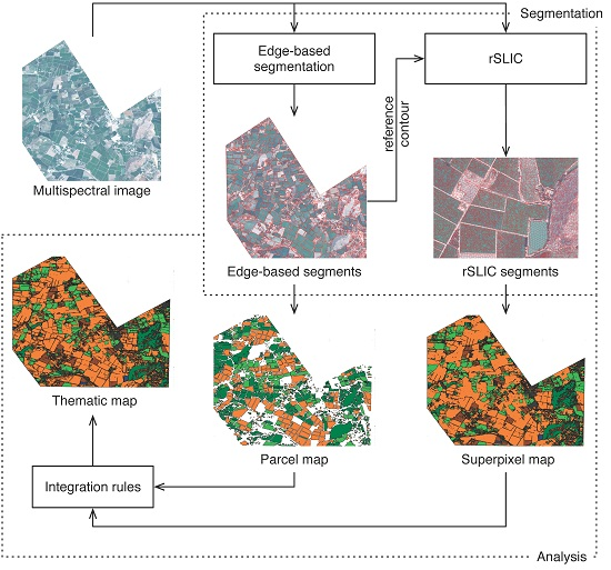
In this paper, we propose an automatic GEOBIA methodology for fragmented agricultural landscapes focusing on the generation of a thematic map of the available classes in the scene. The proposed methodology employs superpixels, instead of image pixels, as minimal processing units of analysis and provides a link between them and meaningful objects (parcels) in order to perform the analysis of the scene. To capture the phenomena (small parcels) occurring at coarser scales (bigger segments), an edge-based method is used to segment the image. A superpixel method, working with the information of based-edge segments (i.e., contours) as basis, is proposed to generate superpixels that exactly correspond with their surface. Superpixel and edge-based scales are used together, in a object-based classification approach, to generate a thematic map that combines both features.
2. Study Area and Dataset
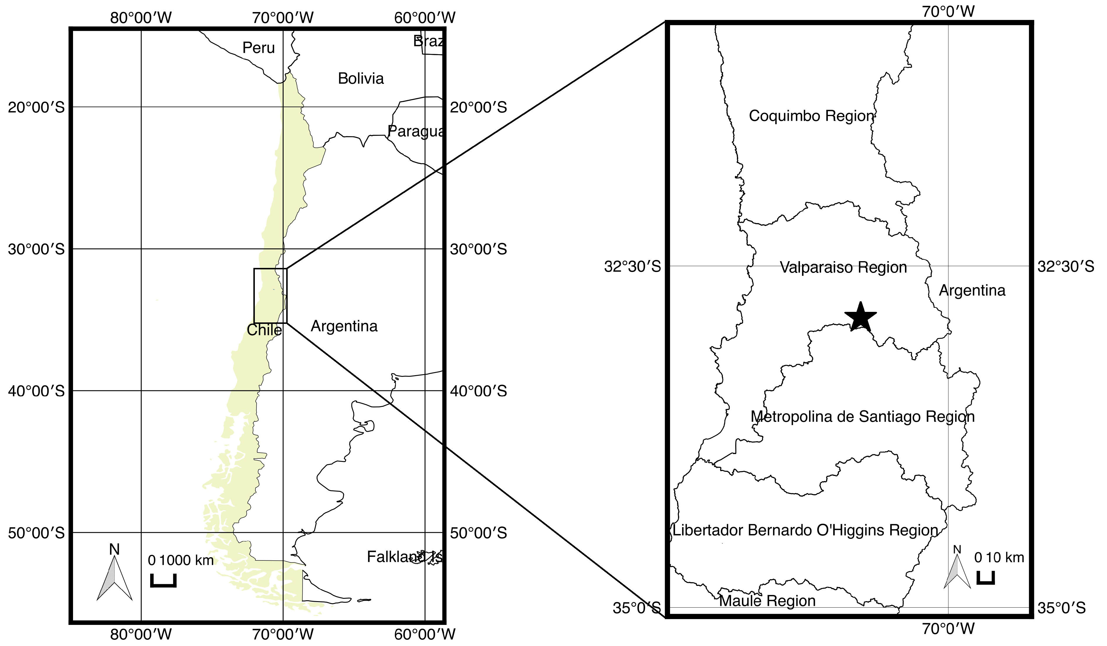
The study area (
Figure 1) corresponds to a Chilean central valley (70°40′7.17′′W, 32°48′11.28′′S), and covers approximately 2660 ha. It is mostly characterized by small agricultural parcels (5 ha on average) with crops of full canopy coverage and orchards. A Quickbird dataset acquired on 3 December 2011, is used for the analysis. The data corresponds to an Ortho-Ready Standard 2A product, and thus has already been radiometric and geometrically corrected. Available panchromatic (PAN) and multispectral (MS) bands are also co-registered. The spectral and spatial properties of the Quickbird image are shown in
Table 1. The full scene has dimensions of 10,217 columns and 10,397 rows in the PAN band.
Figure 1.
The study area is located in Valparaiso Region, Chile. The black star (on the right map) shows the location of the study site.
Figure 1.
The study area is located in Valparaiso Region, Chile. The black star (on the right map) shows the location of the study site.
Table 1.
Spectral properties of the Quickbird image.
Table 1.
Spectral properties of the Quickbird image.
| Band | Spectral Range (µm) | Resolution (m) |
|---|
| blue | 0.45–0.52 | |
| green | 0.52–0.60 | 2.44 |
| red | 0.63–0.69 |
| near-infraread | 0.76–0.90 | |
| PAN | 0.45–0.90 | 0.61 |
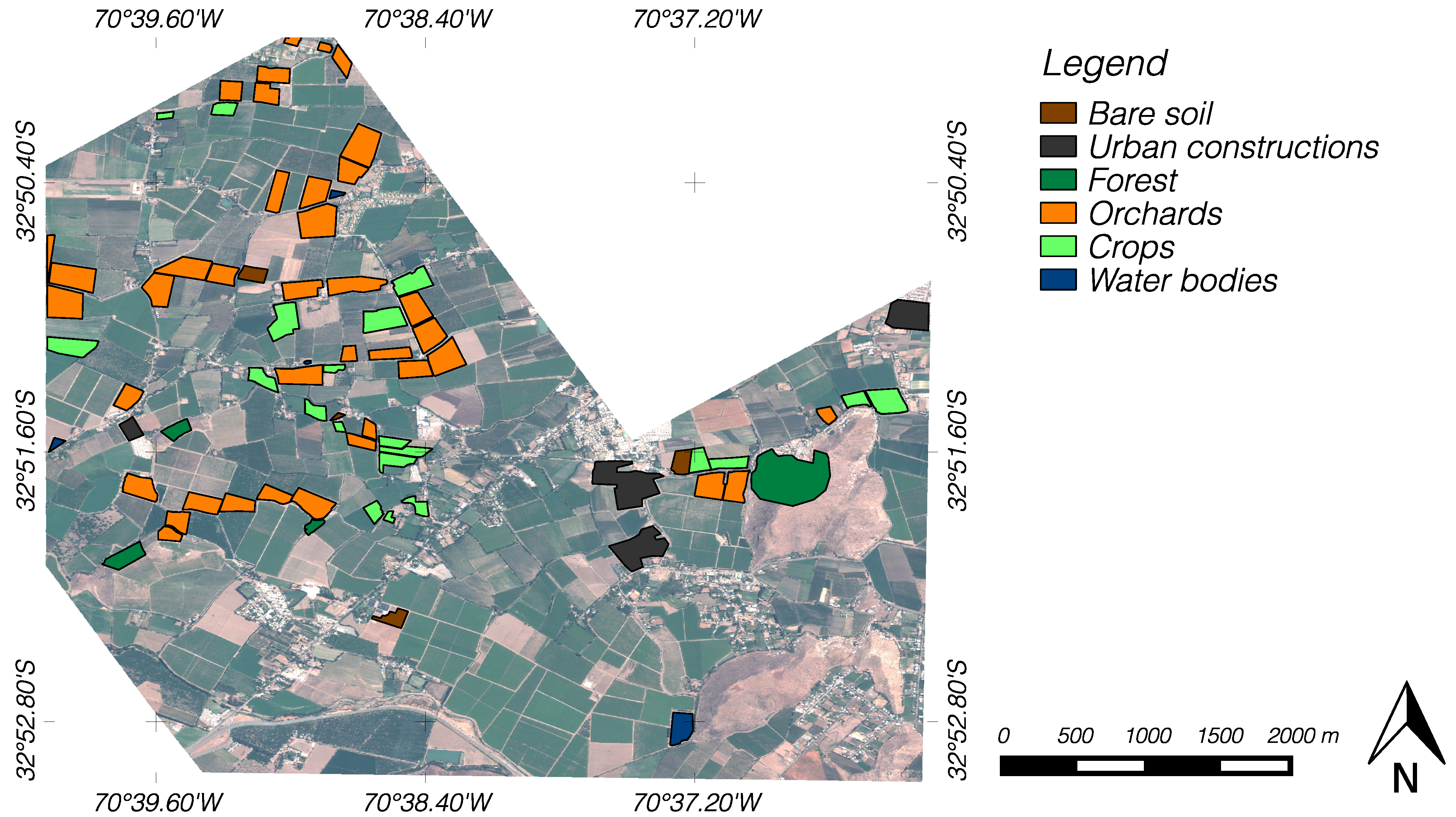
A field campaign was conducted in the study site on the same day of the acquired image to collect information about phenological status of the different land-covers, canopy height and type of planting (partial or full cover). The identified covers in the study area were: bare soil, water bodies, buildings and urban constructions, forest (including shrubs and other natural vegetated areas), and two different types of parcels, crops and orchards. Crops correspond to different types of vegetables and pastures (e.g., alfalfa, maize). Orchards consisted of diverse fruit trees such as nectarines, table grapes, and walnuts, among others. This information was recorded in a GIS vector file and used as ground-truth data for validating the land-covers of interest and the classification results. The polygons included in the vecter file are overlapped to the original image in
Figure 2. The complete distribution of the available ground-truth examples for classification is shown in
Table 2.
Figure 2.
Real color composition (red, green and blue bands) of the Quickbird image. The polygons corresponding to the interest classes are overlapped on the image.
Figure 2.
Real color composition (red, green and blue bands) of the Quickbird image. The polygons corresponding to the interest classes are overlapped on the image.
Table 2.
Class distribution of the available ground-truth examples. The percentage represents the area that covers a class regarding the total area of the ground-truth.
Table 2.
Class distribution of the available ground-truth examples. The percentage represents the area that covers a class regarding the total area of the ground-truth.
| Class | Area (ha) | Percentage (%) |
|---|
| Bare soil | 6.51 | 2.82 |
| Urban constructions | 26.70 | 11.55 |
| Forest | 25.20 | 10.90 |
| Orchards | 123.57 | 53.43 |
| Crops | 44.84 | 19.39 |
| Water bodies | 4.43 | 1.92 |
3. Methodology
In order to automatically analyze VHR images of fragmented agricultural landscapes our methodology combines superpixel processing and edge-based methods, which provide the basis to identify interest objects as parcels and generate land-cover maps. A superpixel method produces a controlled over-segmentation of the image, reducing the intra-variability of the image pixels as well as the size of the analysis space, which allows performing an analysis similar to pixel-based ones. In addition, an edge-based method detects abrupt changes in pixel intensity which usually characterize the object boundaries in a scene. In the case of the images under study, edge-based methods can provide information about the edges corresponding to roads or the limits of parcels, whereas regions within these edges can be obtained by means of low-level image processing operations (e.g., erosion, dilation). These regions are used as a reference for a superpixel method, based on the
Simple Linear Iterative Clustering algorithm (SLIC) [
27], with the premise of the generated superpixels respect boundaries established
a priori. The proposed algorithm, which we have called rSLIC (r stands for reference contours), has two important improvements respect to SLIC method : (1) it works in a multispectral space; and (2) it allows segmenting a specific image region (regardless of its shape) instead of the whole scene.
At superpixel level, a classification step is carried out using the RUSBoost algorithm (
Section 3.2.1) as a classifier, whereas a simple rule-set (
Section 3.2.2) is used at edge-based region level. All processes are carried out using in-house developed codes and run on the MATLAB platform.
3.1. Image Segmentation Scheme
A general scheme of the segmentation process is shown in
Figure 3. This segmentation scheme provides the following working scales: (1) superpixels (finer scale) provide spectral information so they are processed similarly to image pixels; and (2) the edge-based regions (coarser scale) contain edge information in the better case related to parcel boundaries, so they are treated as candidate parcels.
Figure 3.
Segmentation process of a multispectral image. Edge-based segmentation is applied to obtain an initial segmented image. These segments are later used as reference contour by rSLIC to generate superpixels.
Figure 3.
Segmentation process of a multispectral image. Edge-based segmentation is applied to obtain an initial segmented image. These segments are later used as reference contour by rSLIC to generate superpixels.
3.1.1. Edge-Based Segmentation
Physical edges provide important visual information since they correspond to discontinuities in the physical properties of scene objects [
28]. These edges are related to significant variations in the reflectance, illumination, orientation, and depth of scene surfaces. Starting from these edges, regions can be obtained by means of morphological operations such as flood-fill and dilation among others.
The procedure to obtain the regions is described in Algorithm 1. Edges are extracted for each band
b in multispectral image (
MS) using Canny edge detector [
29] (
edge). Then each edge is dilated (⊕), using lines of 3 pixels length in angles of 0 and 90 degrees as structuring element objects (
strel). Only the intersection of all edges is retained in
E, after which all regions and holes of its complement Ẽ are filled using an algorithm based on morphological reconstruction [
30]. The obtained regions
R are dilated, and finally the connected components are labeled using a 4-neighbor connectivity, and resulting in segments
S.
| Algorithm 1: Edge-based segmentation algorithm |
Input: A multispectral image MS.
A morphological structure element strel containing lines in different angles.
Output: A segmented image S.
E = ∅
foreach band b ∈ MS do
![Remotesensing 07 00767 i001]()
Ẽ ← not(max(E))
R ← fill(Ẽ)
R ← dilation(R)
S ← connected − component labeling R
return S |
3.1.2. Superpixel Processing
Superpixel processing is carried out by the rSLIC method, a modified version of the SLIC algorithm which in turn is based on the well-known
k-means method to group pixels of RGB/CIELab (a brief description of the CIELab color space is given by [
31]) images into superpixels. SLIC superpixels are generated according to two criteria: spectral similarity (limited to three channels) and spatial proximity. A detailed description of the SLIC algorithm working in CIELab color space is given by [
27].
In the SLIC procedure, the generation of superpixels is based on the assumption that limiting the search space to a region proportional to the desired superpixel size reduces considerably the calculation time. In fact, its computational complexity is linear in the number of pixels in the image [
17]. Moreover, a weighted distance that combines spectral and spatial proximity allows controlling the size and compactness of the superpixel [
17]. Therefore, it has two parameters:
k, the desired number of superpixels, and
c, the compactness factor. A larger value of
c emphasizes the importance of the spatial proximity resulting in more compact superpixels.
rSLIC extends the definition of spectral proximity provided by SLIC to work with multispectral images of
B bands. The first step of the segmentation framework begins with the sampling of
k initial cluster centers on a regularly spaced grid of
g pixels. The initial centers are defined as:
where
pb represents the spectral value in band
b −
th of pixel
p at position
x and
y, and
B denotes the number of spectral bands. To produce similar sized superpixels, the grid interval is defined as
g =
N/k, where
N is the total number of pixels in the image.
g determines the size of the superpixels, the greater value of
g, the larger the superpixels.
In the next step, each pixel
p is associated to the nearest cluster center whose search space overlaps its location. The search region is enclosed to an area of 2
g × 2
g pixels around each superpixel center. Then the cluster centers are updated to be the mean vector of all pixels belonging to the cluster. Both steps are repeated iteratively until a maximum of 10 iterations, since no further significant changes in superpixel quality could be observed [
27].
The clustering distance is a weighted relationship between spectral and spatial measures. The first measure ensures superpixel homogeneity, and the second one enforces compactness and regularity in superpixels shape. In order to work with multispectral images, the spectral square distance between pixels
i and
j is defined as follows:
The spatial square distance is calculated as:
where
x and
y denote the position of the pixel.
ref corresponds to
a priori shapes, such as the contained in Geographic Information System (GIS) vector layers, which defines specific image regions. Only pixels within
ref are grouped; this improvement allows to generate superpixels in only certain regions rather than the whole scene, slightly reducing runtime in image processing.
Finally, the clustering distance is calculated as:
where
c controls the compactness of the superpixels. Preliminary results suggest that a 3.9% of the maximum pixel value in image as
c is optimal.
3.2. Analysis Scheme
The GEOBIA methodology allows exploiting spatial, shapes, and semantic relations among regions together with their spectral characteristics. As in the works of [
32,
33,
34] the features used for classification are the following:
- Spectral.
Normalized Difference Vegetation Index (NDVI) [
35], Normalized Difference Water Index (NDWI) and Spectral Shape Index (SSI) [
36], as defined in Equations (5)–(7).
where R, B, G and NIR represent the red, blue, green and near-infrared bands, respectively.
- Texture.
Local entropy of an image [
37] computed in a neighborhood of 9
× 9 pixels, and calculated as in Equation (8).
where
zi is a random variable indicating intensity,
p(
z) is the histogram of the intensity levels in a region (usually set to a size of 9),
L is the number of possible intensity levels.
- Shape.
Fractal dimension index (FRAC) [
38], as in Equation (9).
where values greater than 1 indicate an increase in shape complexity.
FRAC approximates 1 for shapes with very simple perimeters such as squares, and approximates 2 for shapes with highly convoluted, plane-filling perimeters.
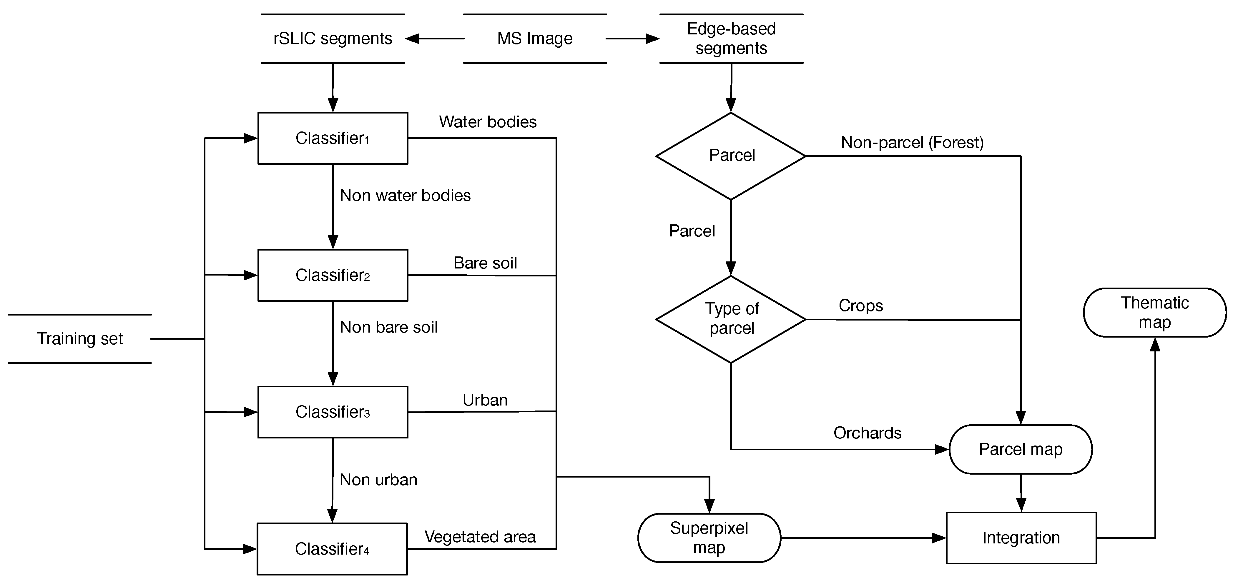
Since two working scales (superpixels and edge-based) are available, different features are used at each analysis scale. Spectral and texture features are extracted from superpixels, whereas shape and texture features are used to characterize edge-based segments. The classification workflow is shown in
Figure 4.
Each superpixel is characterized by the mean and standard deviation of the NDVI, NDWI, and SSI indexes, all the available spectral band values, and the local entropy; and classified according to the following classes: water bodies, buildings and urban constructions, bare soil, and vegetated areas,
i.e., forest, crops, and orchards. Because the PAN band contains more information about texture, local entropy is calculated from it. Then a dataset is created using characterized superpixels as observations. These are labeled according to an overlap criteria: if at least 80% of a superpixel surface coincides with the surface of a ground-truth region, then the corresponding observation acquires the label of this region. Because superpixels are similar in size and well adapted to image regions, the labeled subset follows the same distribution as the ground-truth dataset (see
Table 2). This new dataset is used for classification. Since this dataset is imbalanced, a classifier that considers the distribution of the class is needed in order to obtain satisfactory results. For this reason, the RUSBoost algorithm [
39], described in
Section 3.2.1, is used as classifier.
A cascade multi-staging classification of superpixels is conducted. In each stage, a classification is performed using RUSBoost classifier over only two classes, which are defined as the dichotomic relationship between an interest class and the rest of them. For example, when the class under study corresponds to water bodies, the other class includes everything (i.e., bare soil, urban constructions, and vegetated areas) that has not been previously classified. This classification scheme is inspired by land-cover taxonomies (e.g., CORINE Land-cover scheme), where dichotomic categorizations are followed by experts to generate standardized thematic maps.
Figure 4.
Workflow of the analysis process. Two classifications are carried out over superpixels and edge-based regions. The first one considers spectral and texture features. The second one employs shape and texture features, as well as the information provided by the previous classification to generate a final thematic map.
At edge-based segments scale, fractal dimension index (Equation (9)) is used to distinguish which segments could be parcels from natural entities as forests in the whole segmented image. Therefore regions where
FRAC approximates 1 are considered as candidate parcels, whereas segments with higher values are considered as forests. Because of their planting frame (the way how trees are planted), orchards present a high variability, whereas crops are more homogeneous respect to its gray values. To classify which parcels are potentially crops or orchards, local entropy is calculated from the PAN band and each segment is then characterized and analyzed. This analysis is performed using a rule-based classification (
Section 3.2.2).
From the analysis of superpixels and edge-based segments, maps at superpixel and parcel scales are respectively generated. The former one is obtained from data-driven methods using ground-truth land-cover data and information provided by the edge-based regions of the parcels. Superpixel map provides information about different interest classes and not about parcels (interest objects) in the image. On the other hand, the parcel map provides information about parcel candidate segments using the rules based on shape and texture attributes. However, they do not supply information about land-cover classes on images.
An integration process is performed to merge both the information superpixels and parcel maps. The composition is made analyzing each segment at a parcel scale, by means of the classified superpixels which form part of it. A parcel segment is labeled according to the vegetated region, on a superpixel map that covers most of its surface following the next condition: if the majority label agrees with the classification on the parcel map, then the entire parcel segment keeps its label. But if a discrepancy arises between both classifications, the segment is marked as incongruent. Two types of incongruent segments are considered:
- Type 1 (T1).
These are vegetated regions that according to their shape were considered as non-parcels. However, they are classified as orchards or crops at superpixel level.
- Type 2 (T2).
These are segments whose classes in both maps are interchanged, e.g., on the parcel map, a segment is identified as an orchard. However, the overlapping region is classified as crops on the superpixel map.
In order to provide an automatic solution to incongruent segments, two criteria are established to substitute T1 and T2. In the case of T1 segments, they are replaced by the overlapping areas on the superpixel map, due to the possibility that at a superpixel scale the region could be divided by different land-covers into smaller parts with a more regular shape. On the other hand, T2 segments are labeled according to the majority vegetated class (orchards or crops) covering its surface at superpixel level. The information of the superpixel map, instead of the given by the parcel map, is primarily used for labeling a T2 segment because the rule used to labeled it could be far too restrictive for some parcels in an incipient vegetative stage.
3.2.1. RUSBoost Classifier
RUSBoost is a hybrid boosting/sampling method proposed by [
39], which is a state-of-the-art method for learning from imbalanced datasets [
40]. RUSBoost improves boosting algorithm by resampling training data in order to balance the class distribution.
RUSBoost is based on SMOTEBoost [
41], which in turn is based on the AdaBoost.M2 algorithm [
42]. Unlike other ensemble methods RUSBoost applies RUS as under-sampling strategy to randomly remove samples from the majority class, before the training of each weak learner algorithm that is part of the ensemble. This reduces the total time of training without performance loss [
39].
RUSBoost combines an under-sampling technique, known as RUS, with AdaBoost.M2 algorithm. AdaBoost.M2 is an ensemble method for multi-class classification. It combines many weak classifiers
ht into a strong classifier
H by linear combination. The final classifier is constructed as:
The resulting class
y, given the input feature vector
x, is the one that gets the maximum value. The weak learners are added incrementally to
H . In each iteration
t, RUSBoost applies RUS to randomly subsample the majority class in training set
X until a subset
X't with a desired class distribution is reached. For example, if the desired class ratio
r is 50:50, then the majority class examples are randomly removed until the numbers of majority and minority class examples are equal. Hence a weight
αt is assigned to the weak learner according to the relation:
where
ϵt represents the pseudo-loss based the original training set
X and a weight distribution
Dt for all examples in
X and is calculated as:
where
ht(
xi, y) represents the conditional probability of the class
y given the feature vector
xi∈
X .
Initially, the weight of each example
D1(
i) is set to 1
/n where
n is the number of examples in the training set. After each iteration, the weights are updated as follow:
and then
Dt+1 is normalized to 1.
3.2.2. Rule-Based Classification
Information about regularity of the shape is used as a feature to distinguish which segments could be parcels from natural entities as forests in the whole segmented image. Following the definition of fractal dimension index (Equation (9)), regions with a shape value around 1 are considered regular whereas higher values are complex forms. Thus a simple rule based on segment shape is defined to distinguish between parcels (orchards and crops) and non-parcels:
Once candidate parcels are obtained, they are analyzed by their textural characteristics. Because of the way the trees are planted (planting frame), orchards have high texture compared to crops. Therefore, a rule to differentiate these types of parcels was formulated as follows:
4. Results and Discussion
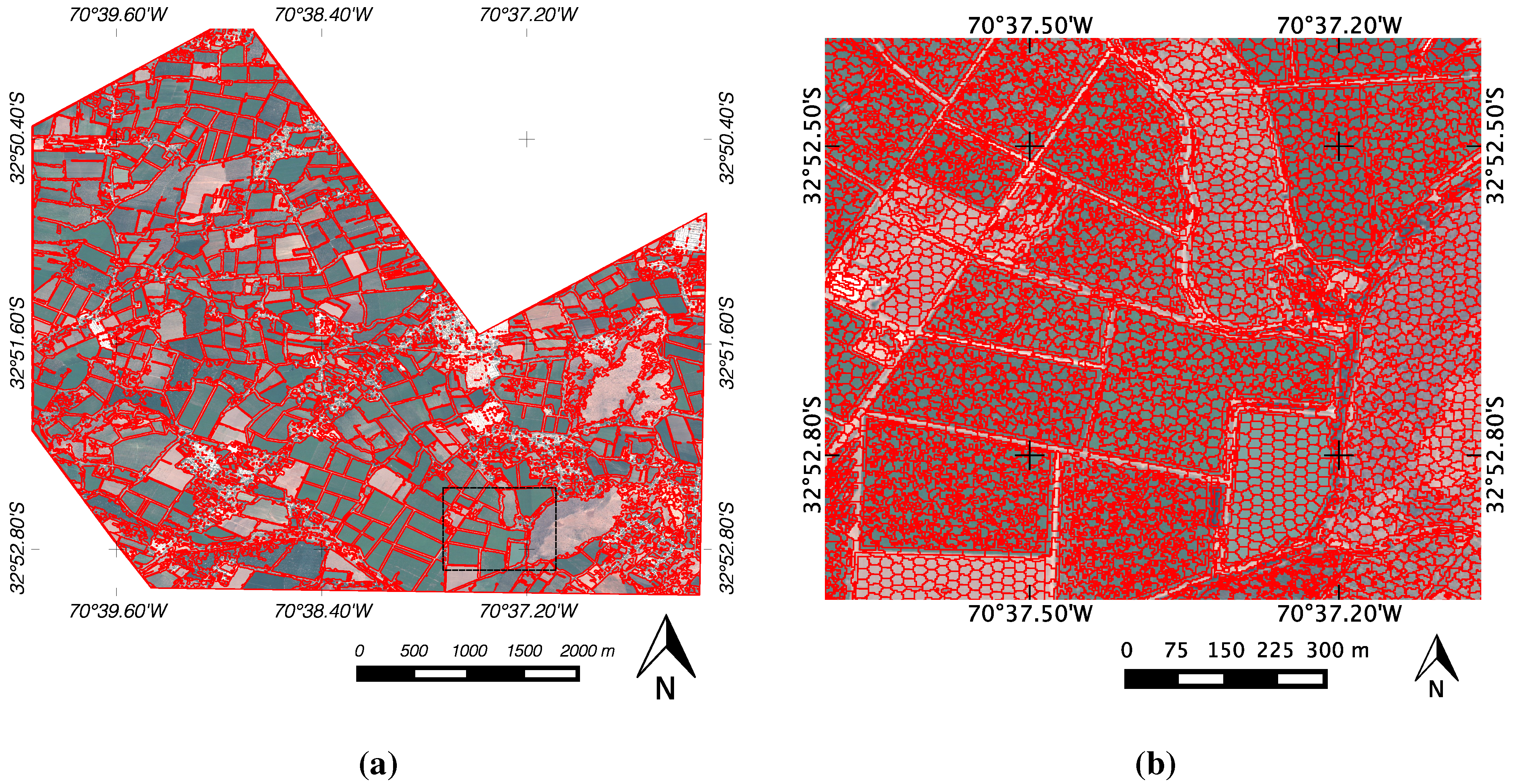
From multispectral bands, two segmented images were obtained by using edge-based and rSLIC methods. As shown in
Figure 5a, edge-based segments are well suited to most of the small agricultural parcels. From these segments, using a compactness factor of 80, a total of 297,257 superpixels covering the whole image were automatically generated, where each superpixel is composed of 25 pixels on average. They represent 4% of observations to analyze respect to the entire number of image pixels under analysis. The inclusion of edge-based segments as
a priori information for rSLIC algorithm allows segmentation inside of specific areas, which is useful for intra-parcel analysis. As can be observed, superpixels respect the limits of the edge-based segments and adhere well to the boundaries of spectrally homogeneous regions. Due to visualization issues, only a zooming-in image region containing a set of generated superpixels is shown in
Figure 5b.
Figure 5.
The edge-based segmentation (
a) provides regions whose edges (red lines) mark the location of discontinuities in color as the roads. The result of rSLIC (
b) shows regions of slightly different shapes according to the spectral properties of the image, but following and preserving the edges previously obtained.
Figure 5b corresponds to the area enclosed by the black dotted square marked in
Figure 5a.
During the superpixel multistage classification, at each stage, a total of 1000 decision trees were used as weak learners (
h) to build a single RUSBoost classifier using a ratio of sampling
r of 50:50. To validate classification results a 3-fold cross validation was performed by an image object assessment. That means that the statistics are calculated over the given classes to superpixels (image objects) corresponding to the test set in each fold. The obtained results show mean accuracies (user and producer) greater than 88% with a small deviation standard (1.36 on average) for all classes except for the bare soil class, where the user accuracy is 58.37%. In addition, the results point out a commission error of 63.40% for the same class. This may occur because entities identified by experts as parcels and forests are not completely pure,
i.e., they can contain heterogeneities such as patches of bare soil. In spite of that fact, the obtained results can be considered competitive and stable, since they are high (averages of 88% and 91% for user and producer accuracies, respectively) and present a low variability (an average lower than 1.6 in both cases). The assessment of multi-staging classification at superpixel level is displayed in
Table 3.
After the classification step, a superpixel map is generated integrating the superpixels classified by the classifier with the best accuracy score.
Figure 6 shows the result of the classification at superpixel level. As can be observed, even though the generated superpixel map does not present adverse outcomes as a
salt-and-pepper effect, not all parcels are represented as homogeneous areas, since some of them mostly contain small bare soil regions. Likewise, the same occurs with bare soil regions where small vegetated regions are presented. This agrees with reality since parcel homogeneity depends on various factors, such as management practices, soil properties, among others. Moreover, adjacent orchards separated only by dirt roads are joined together, making it impossible to distinguish one parcel from another. In
Table 4, the confusion matrix of the classification map is presented. Therein can be observed the heterogeneity phenomena among vegetated areas and bare soil, but also among forests, crops and orchards. To validate current and subsequently generated maps, an accuracy assessment based on random points was performed. An overall accuracy of 91.74% and a Cohen’s kappa coefficient (
κ) of 0.8728 are obtained by comparing the ground-truth data and the superpixel map. The above implies that information given to the classifier is not enough to completely separate the classes, and that more information needs to be added. For this purpose, edge-based segments are incorporated to the process.
Table 3.
Accuracy assessment of the classification at superpixel level.
Table 3.
Accuracy assessment of the classification at superpixel level.
| Classes | User Acc. (%) | Prod. Acc. (%) | Comm. (%) | Omm. (%) |
|---|
| Water bodies | 96.56 ± 3.11 | 89.73 ± 1.11 | 3.20 ± 2.93 | 10.21 ± 1.11 |
| Bare soil | 58.37 ± 1.57 | 88.76 ± 2.22 | 63.40 ± 11.06 | 11.06 ± 2.22 |
| Urban constructions | 95.22 ± 0.72 | 90.70 ± 1.30 | 4.55 ± 0.76 | 9.22 ± 1.30 |
| Forest | 88.75 ± 1.11 | 89.75 ± 0.66 | 11.36 ± 1.25 | 10.23 ± 0.66 |
| Crops | 91.13 ± 1.39 | 90.20 ± 1.62 | 1.67 ± 0.27 | 1.4 ± 0.28 |
| Orchards | 98.32 ± 0.26 | 98.49 ± 0.28 | 8.79 ± 9.70 | 9.70 ± 1.62 |
Figure 6.
Superpixel map generated through the classification of superpixels according to the interest classes.
Figure 6.
Superpixel map generated through the classification of superpixels according to the interest classes.
Table 4.
Confusion matrix showing results of the classification at superpixel level. The values are expressed on percentages of overlapping area between superpixels andground-truth regions.
Table 4.
Confusion matrix showing results of the classification at superpixel level. The values are expressed on percentages of overlapping area between superpixels andground-truth regions.
| | Classification | |
|---|
| Ground-Truth Areas | Water | Bare Soil | Urban | Forest | Orchards | Crops | Total |
|---|
| Water | 94.83% | 0.72% | 0.23% | 3.61% | 0.53% | 0.09% | 100% |
| Bare soil | 0.00% | 87.72% | 0.70% | 3.09% | 3.16% | 5.33% | 100% |
| Urban | 0.00% | 1.88% | 87.39% | 4.70% | 5.35% | 0.69% | 100% |
| Forest | 0.00% | 5.90% | 8.52% | 79.07% | 6.23% | 0.29% | 100% |
| Orchards | 0.01% | 0.28% | 0.17% | 2.45% | 95.97% | 1.13% | 100% |
| Crops | 0.00% | 1.74% | 0.71% | 0.04% | 7.42% | 90.09% | 100% |
| Total | 94.84% | 94.84% | 97.71% | 92.95% | 118.65% | 97.61% | |
Edge-based segments provide a working scale closely related to the boundaries of the parcel (interest objects). Therefore, they are used to generate additional information in order to improve the results of vegetated areas (i.e., forests, crops and orchards) at superpixel scale. It should be remarked that obtaining these segments only depends on low-level image processing operations (e.g., erosion, flood filling, dilation), so regions are generated without the necessity of fine-tuning any parameter. Inasmuch as edge-based regions are used as candidate parcels, high level descriptions of them are used to determine which segments are more likely to be orchards or crops.
These segments were classified using the rules defined in
Section 3.2.2. For Equation (14), thresholds were empirically selected to distinguish regular segments. In this paper, a
FRAC value in a range of 1 ± 0.1 are considered as candidate parcels. Therefore,
thfrac1 and
thfrac2 were set to 0.9 and 1.1, respectively. To discriminate orchards and crops
thentropy is set to 4, a value obtained through sampling of the texture image. During this analysis, only segments that contain at least a surface covered 60% by vegetation (on the superpixel map) are considered to be analyzed.
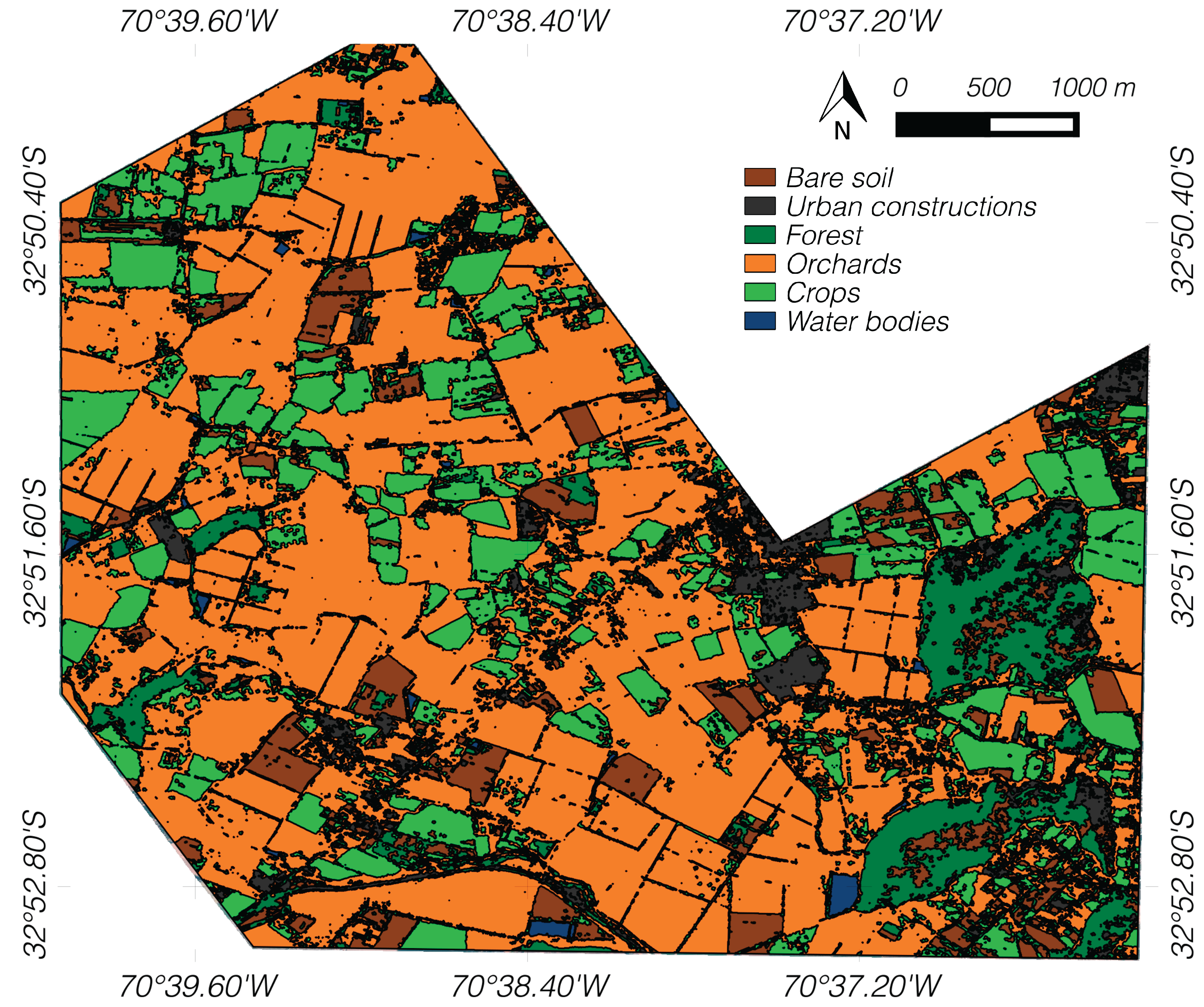
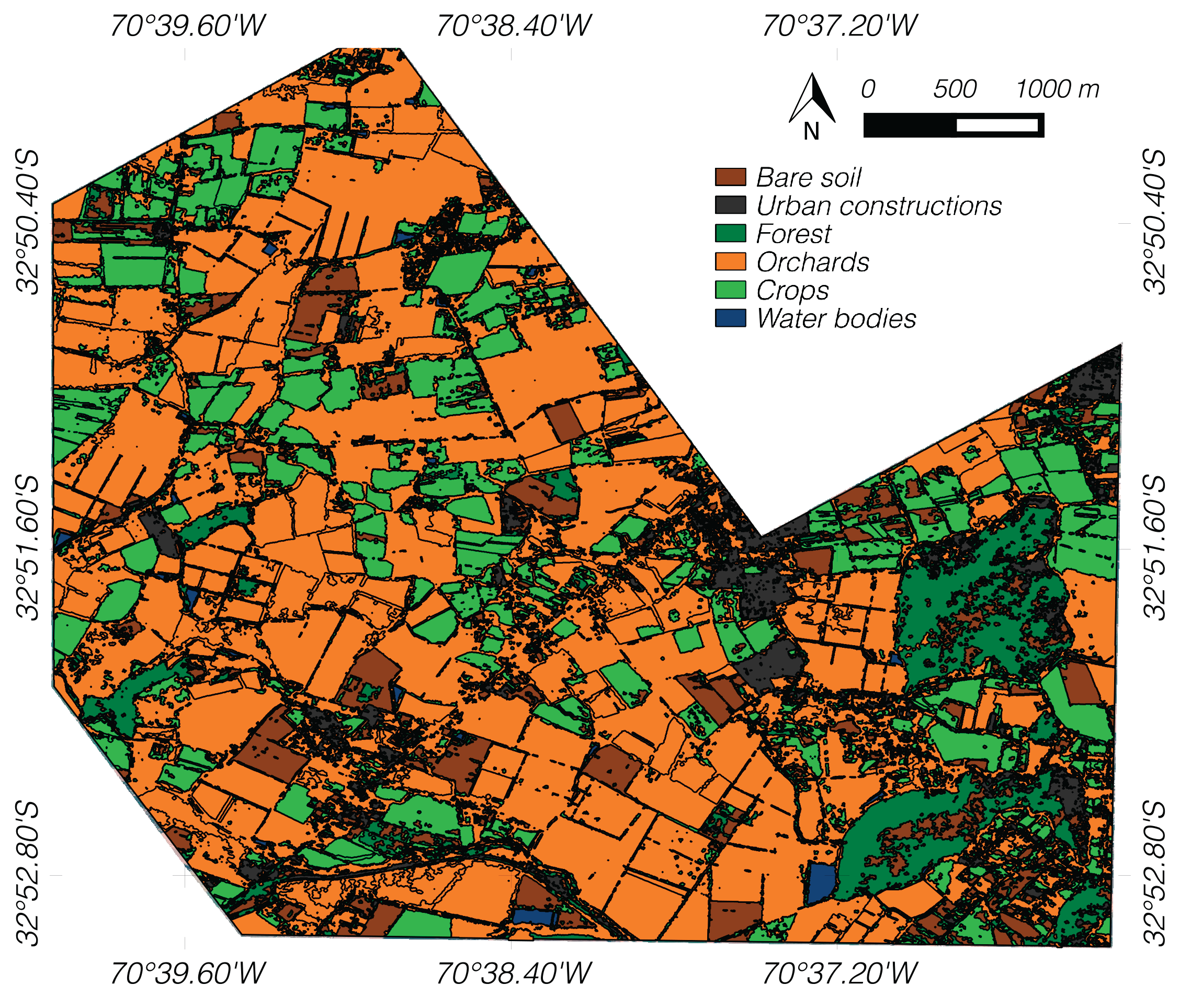
The result of applying the rules at edge-based segments level is shown in
Figure 7. The obtained map, called parcel map, shows vegetated areas likely to be parcels separated from others areas trough the use of a shape feature. Crops and orchards are differentiated using the texture characteristics of the candidate parcels.
The integration of information of both superpixel and parcel maps is displayed in
Figure 8. The regions of
T1 and
T2 are represented in two gray-scale colors. As can be observed, identified parcels on the resulting map represent only one land-cover, as opposed to superpixel maps where the regions inside parcels could contain more than one type of land-cover. This behavior is similar to the analysis done by human operators, where heterogeneities are often not considered when making the delimitation of land-covers. In general,
T1 regions mainly occur on segments that were incorrectly delimited at a parcel scale. Therefore, an improvement in the delimitation of the object is probably required. This is potentially useful for
T2 regions, which mainly arise because it is difficult to discriminate between classes in the parcels when vegetation is at an early phenological stage. In spite of that fact, information about the composition of a specific parcel is useful for intra-parcel analysis, so this information can be accessed through the superpixels that form part of it. Moreover, superpixels entirely provide the information about the non-vegetated areas (e.g., water, bare soil), whereas incongruent segments (
T1 and
T2) give information about regions that require a disambiguation by an expert.
Figure 7.
Map of the vegetated areas. Two types of parcels are distinguished among them and from other vegetated areas using shape and texture characteristics.
Figure 7.
Map of the vegetated areas. Two types of parcels are distinguished among them and from other vegetated areas using shape and texture characteristics.
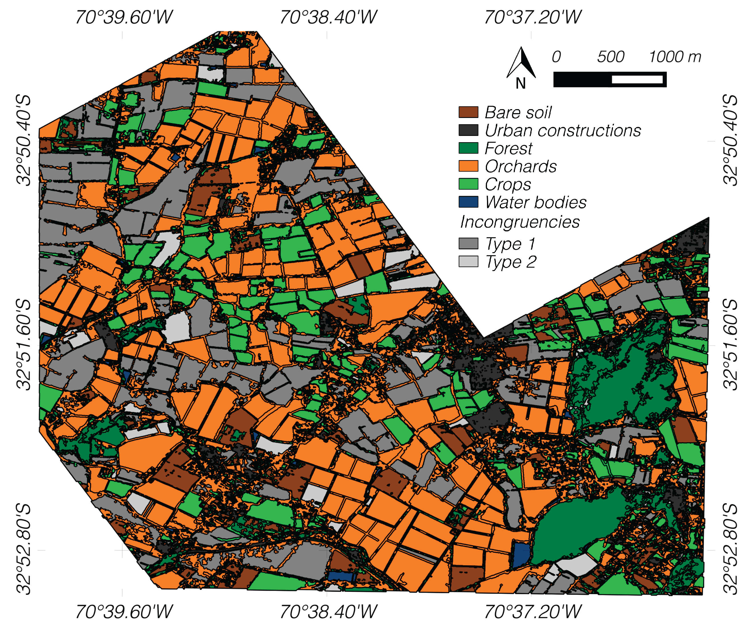
Figure 8.
Combination of superpixel and parcel maps. In two different gray-levels, incongruent regions between parcel and superpixel maps are shown.
Figure 8.
Combination of superpixel and parcel maps. In two different gray-levels, incongruent regions between parcel and superpixel maps are shown.
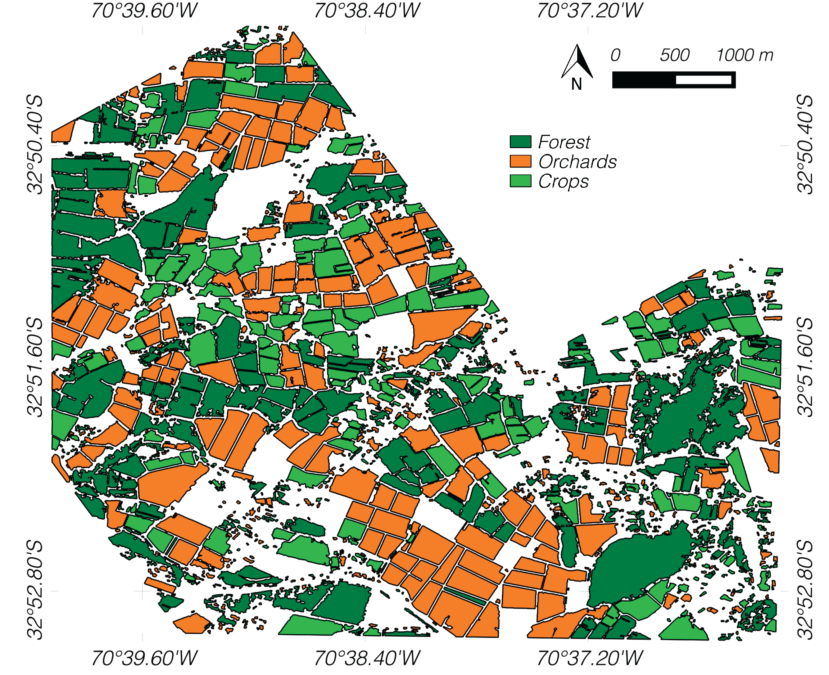
The result of applying the criteria to substitute
T1 and
T2 segments by a vegetative ground-truth class is displayed in
Figure 9. The final map has a
κ value of 0.8947 and an overall accuracy of 93.25%. These results show an improvement in classification compared to the obtained in superpixel maps. Moreover, in the confusion matrix (
Table 5), a refinement of vegetative classes is observed, especially in the forests (shrubs and natural vegetated areas) class where an increment of accuracy, from 79.04% to 86.61%, is reached. This occurs because giving a unique label for entire parcel area reduces the intra-variability of the map. Therefore, some heterogeneities (e.g., bare soil regions) are eliminated in better agreement with the ground-truth data in natural vegetated areas. Conversely, a slight decrease in accuracy, respect to the superpixel map, can be seen in the bare soil (−4.03%) and urban classes (−0.04%). This phenomenon mainly occurs at the edges of both classes that are adjacent to a vegetated area, which implies that there is a slight mismatch between some segments and the objects defined in the ground-truth data.
Figure 9.
Final map generated with the disambiguation of T1 and T2 regions.
Figure 9.
Final map generated with the disambiguation of T1 and T2 regions.
Table 5.
Confusion matrix showing results of the classification of the final map. The values are expressed on percentages of overlapping area between ground-truth regions and the final map.
Table 5.
Confusion matrix showing results of the classification of the final map. The values are expressed on percentages of overlapping area between ground-truth regions and the final map.
| | Classification | |
|---|
| Ground-Truth Areas | Water | Bare Soil | Urban | Forest | Orchards | Crops | Total |
|---|
| Water | 94.83% | 0.72% | 0.23% | 3.61% | 0.53% | 0.09% | 100% |
| Bare soil | 0.00% | 83.69% | 0.00% | 4.35% | 4.45% | 7.51% | 100% |
| Urban | 0.00% | 1.88% | 87.35% | 4.64% | 5.40% | 0.74% | 100% |
| Forest | 0.00% | 0.93% | 4.35% | 86.61% | 7.93% | 0.18% | 100% |
| Orchards | 0.00% | 0.12% | 0.17% | 0.86% | 96.15% | 2.70% | 100% |
| Crops | 0.00% | 0.01% | 0.01% | 0.02% | 6.63% | 93.32% | 100% |
| Total | 94.83% | 87.35% | 92.11% | 100.08% | 121.09% | 104.54% | |
5. Conclusions
In this paper, a methodology based on superpixels for landscapes dominated by small agricultural parcels has been presented. The methodology incorporates two scales of analysis: superpixels and edge-based scale. They are made using an improved version of the Simple Linear Iterative Clustering algorithm (herein proposed and called rSLIC) and an edge-based procedure, for generating superpixels and segments closer to parcels, respectively.
The analysis of both scales allows the acquisition of different types of information about the landscape. On the one hand, superpixel analysis provides information about the scene at a scale more related to image pixels, but with the advantage of reducing the analysis space and image variability, and consequently, the processing time (supervised classification step). Moreover, the use of image edges as a priori information for the generation of superpixels allows to obtain regions with well-defined borders. On the other hand, the edge-based segmentation method provides segments closer to real parcels with no need of a time-demanding tuning process, since they are automatically generated. Even if some parcels are not perfectly delimitated, edge-based segments are useful for the analysis of forms. This allows determining which regions require a more detailed analysis and which ones are candidates for being parcels. Both methods are easily automated, since only a few parameters are required, i.e., only two in the case of the superpixel method, which is useful for the automation of the image analysis.
The combination of the information of both scales provides an automatic way to obtain a thematic map with characteristics of superpixels and candidate parcels. The map presents homogeneous appearance in vegetated areas, whereas heterogeneity is maintained through superpixels for non-vegetated areas. The methodology was tested using a scene with agricultural fragmented landscape. The use of two complementaries methods (rSLIC and edge-based) achieves a classification accuracy better than when those methods are performed separately.


 ,
, 


