
Modeling Aboveground Biomass in Dense Tropical Submontane Rainforest Using Airborne Laser Scanner Data

 ,
,
Abstract
:
1. Introduction
2. Material and Methods
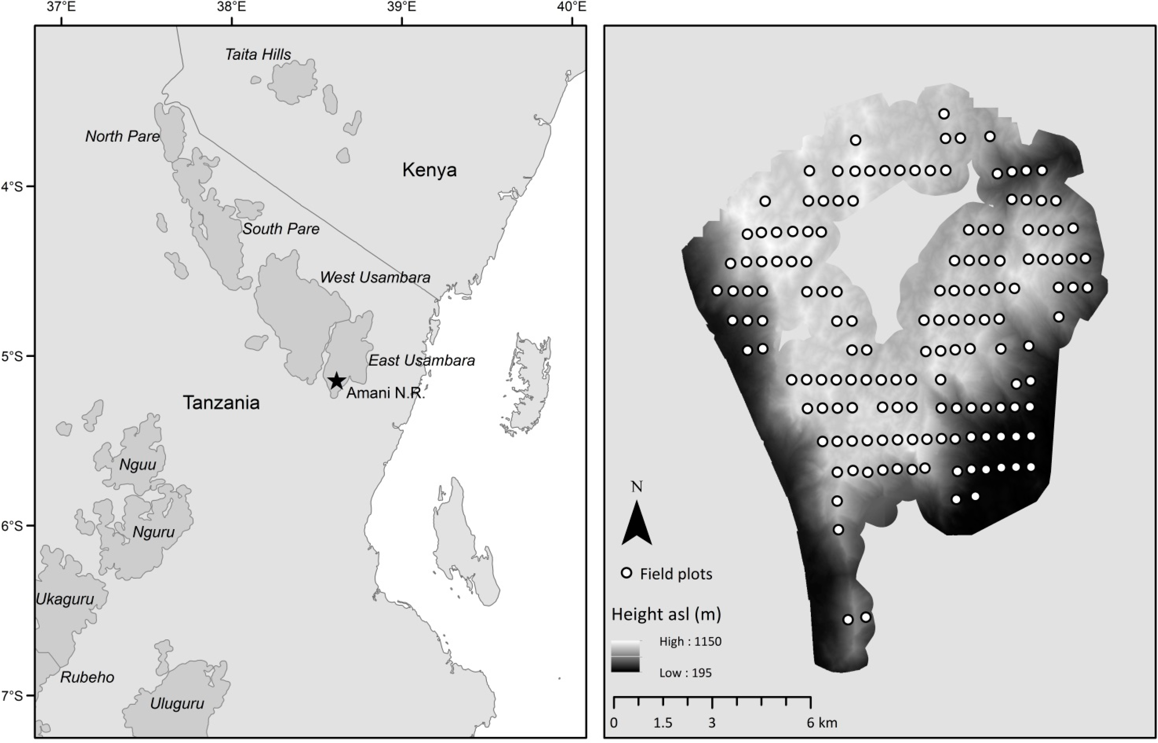
2.1. Study Area

2.2. Field Data

| Characteristic | Range | Mean | SD |
|---|---|---|---|
| Area (ha) | 0.0639–0.1239 | 0.0914 | 0.011 |
| N a (ha−1) | 85.4–1085.7 | 471.5 | 161.5 |
| DBH b (cm) | 10.0–270.0 | 27.5 | 22.9 |
| BA c (m2·ha−1) | 5.4–144.9 | 47.3 | 22.2 |
| AGB d (Mg·ha−1) | 43.2–1147.1 | 461.9 | 214.7 |
| H e (m) | 8.3–51.3 | 19.2 | 8.9 |
2.2.1. Height-Diameter Models
| Variable | Parameter estimate | SD |
|---|---|---|
| a | 0.3376 | (0.9032) |
| b | 0.9834 | (0.0855) |
| c | 0.0172 | (0.0012) |
| 4.9221 | ||
| 0.5905 | ||
| 0.0024 | ||
| 0.3485 | ||
| pR2 | 0.75 | |
| RMSE | 5.38 |
2.2.2. Aboveground Biomass
2.2.3. Positioning of the Field Plots
2.3. ALS Data
2.4. Multiple Regression Analysis
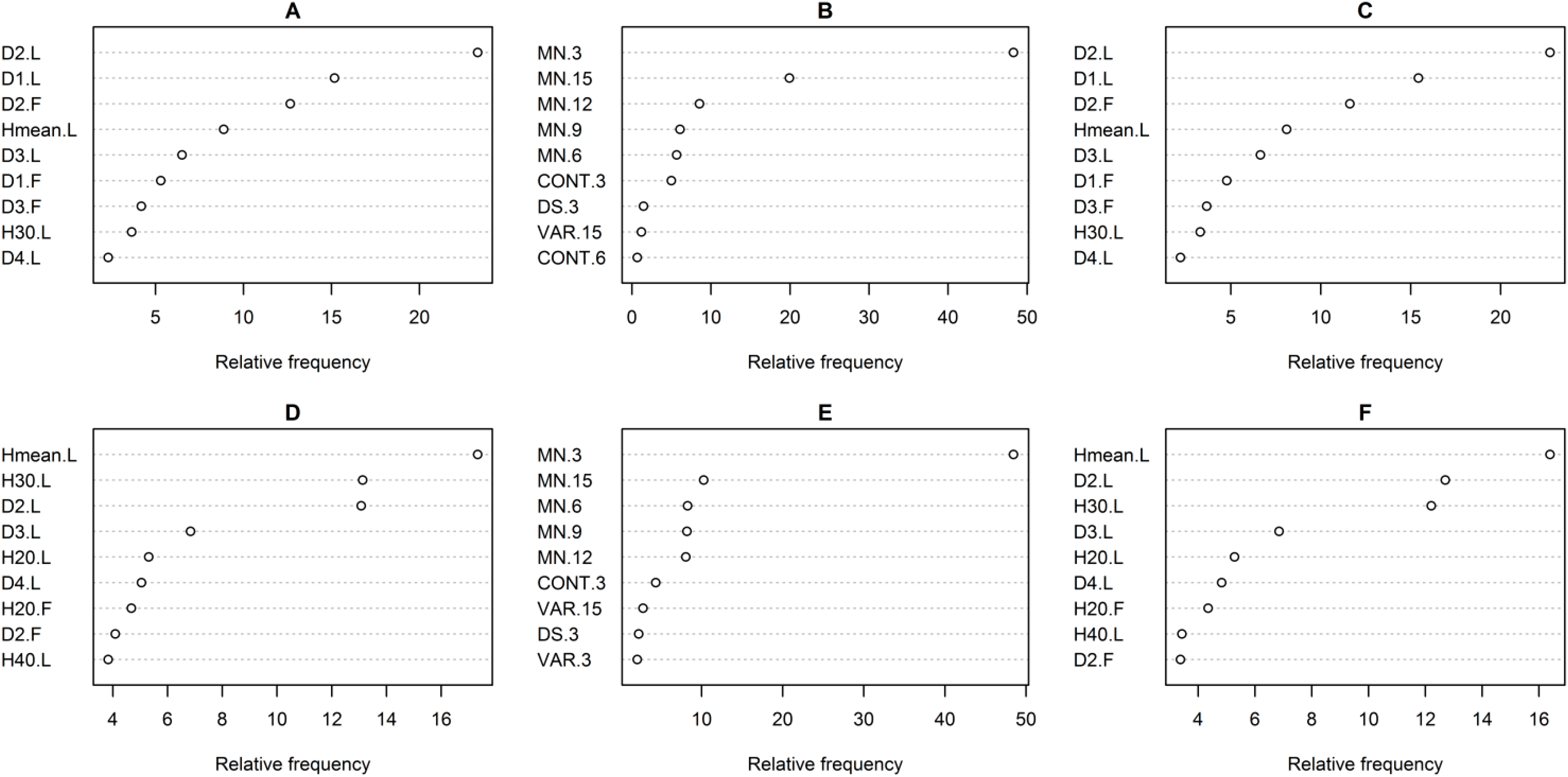
| Model | Transformation | Predictor variables |
|---|---|---|
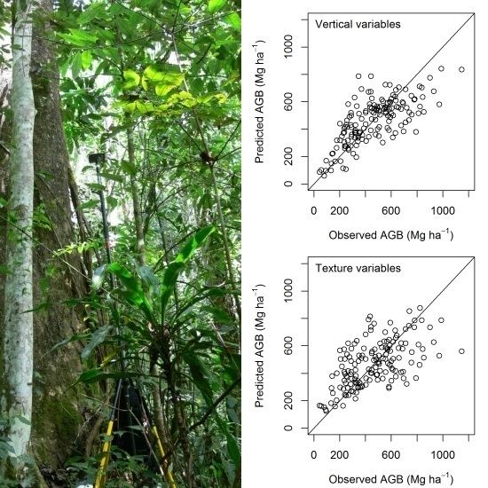
| A | Logarithmic | Vertical |
| B | Logarithmic | Texture |
| C | Logarithmic | Vertical + Texture |
| D | Square root | Vertical |
| E | Square root | Texture |
| F | Square root | Vertical + Texture |
2.5. Analysis of ALS Variables
3. Results
| Model | Response Variable | Predictive Model a | Model Fit | 10-Fold Cross-Validation b | ||||||
|---|---|---|---|---|---|---|---|---|---|---|
| R2 | BIC | RMSE | RMSE% | % | ||||||
| A | ln AGB | 3.815 + 1.755 D2.L+ 1.498·D9.L + 0.016 H90.F | 0.70 | 98.8 | 149.18 | 32.3 | −2.40 | 0.5 | ||
| B | ln AGB | 3.984 + 3.222 MN.3 | 0.52 | 160.6 | 173.84 | 37.6 | −8.57 | 1.9 | ||
| C | ln AGB | 3.665 + 1.530 D2.L + 1.231·D9.L + 0.013 H90.F+ 0.737 MN.15 | 0.71 | 98.7 | 158.02 | 34.4 | −2.85 | 0.6 | ||
| D | sqrt(AGB) | 3.796 + 11.294 D2.L + 13.321·D9.L+ 0.249 Hmean.L | 0.62 | 814.4 | 154.44 | 33.4 | 6.12 | 1.3 | ||
| E | sqrt(AGB) | 7.563 + 0.054 MN.3 − 0.072·CONT.3 | 0.48 | 857.0 | 169.77 | 36.8 | 8.17 | 1.8 | ||
| F | sqrt(AGB) | 3.796 + 11.294 D2.L + 13.321·D9.L + 0.249 Hmean.L | 0.62 | 814.4 | 156.59 | 33.9 | 5.57 | 1.2 | ||


4. Discussion
5. Conclusions
Acknowledgments
Author Contributions
Conflicts of Interest
References
- Lewis, S.L.; Sonké, B.; Sunderland, T.; Begne, S.K.; Lopez-Gonzalez, G.; van der Heijden, G.M.F.; Phillips, O.L.; Affum-Baffoe, K.; Baker, T.R.; Banin, L.; et al. Above-ground biomass and structure of 260 African tropical forests. Philos. Trans. Royal Soc. B Biol. Sci. 2013, 368. [Google Scholar] [CrossRef] [Green Version]
- Bastiaanssen, W.; Noordman, E.; Pelgrum, H.; Davids, G.; Thoreson, B.; Allen, R. SEBAL model with remotely sensed data to improve water-resources management under actual field conditions. J. Irrig. Drain. Eng. 2005, 131, 85–93. [Google Scholar] [CrossRef]
- De Jong, S.M.; Jetten, V.G. Estimating spatial patterns of rainfall interception from remotely sensed vegetation indices and spectral mixture analysis. Int. J. Geogr. Inf. Sci. 2007, 21, 529–545. [Google Scholar] [CrossRef]
- Doherty, R.M.; Sitch, S.; Smith, B.; Lewis, S.L.; Thornton, P.K. Implications of future climate and atmospheric CO2 content for regional biogeochemistry, biogeography and ecosystem services across East Africa. Glob. Change Biol. 2010, 16, 617–640. [Google Scholar] [CrossRef]
- ITTO (International Tropical Timber Organization). Annual Report 2012; ITTO: Yokohama, Japan, 2012. [Google Scholar]
- Masera, O.; Ghilardi, A.; Drigo, R.; Angel Trossero, M. WISDOM: A GIS-based supply demand mapping tool for woodfuel management. Biomass Bioenergy 2006, 30, 618–637. [Google Scholar] [CrossRef]
- UNFCCC. Report of the Conference of the Parties on Its Sixteenth Session, Held in Cancun from 29 November to 10 December 2010. Addendum. Part Two: Action Taken by the Conference of the Parties at Its Sixteenth Session; United Nations Office: Geneva, Switzerland, 2011; p. 31. [Google Scholar]
- UNFCCC. Outcome of the Work of the Ad Hoc Working Group on Long-Term Cooperative Action under the Convention—C. Policy Approaches and Positive Incentives on Issues Relating to Reducing Emissions from Deforestation and Forest Degradation in Developing Countries and the Role of Conservation, Sustainable Management of Forests and Enhancement of Forest Carbon Stocks in Developing Countries; United Nations Office: Geneva, Switzerland, 2010. [Google Scholar]
- UNFCCC. Report of the Conference of the Parties on Its Fifteenth Session, Held in Copenhagen from 7 to 19 December 2009. Addendum. Part Two: Action taken by the Conference of the Parties at Its Fifteenth Session; United Nations Office: Geneva, Switzerland, 2010; p. 43. [Google Scholar]
- UNFCCC. Good Practice Guidance and Adjustments Under Article 5, Paragraph 2, of the Kyoto Protocol; FCCC/KP/CMP/2005/8/Add.3 Decision 20/CMP.1; United Nations Office: Geneva, Switzerland, 2006. [Google Scholar]
- Grassi, G.; Monni, S.; Federici, S.; Achard, F.; Mollicone, D. Applying the conservativeness principle to REDD to deal with the uncertainties of the estimates. Environ. Res. Lett. 2008, 3. [Google Scholar] [CrossRef]
- Gibbs, H.K.; Brown, S.; Niles, J.O.; Foley, J.A. Monitoring and estimating tropical forest carbon stocks: making REDD a reality. Environ. Res. Lett. 2007, 2. [Google Scholar] [CrossRef]
- Plugge, D.; Baldauf, T.; Köhl, M. Reduced Emissions from Deforestation and Forest Degradation (REDD): Why a robust and transparent Monitoring, Reporting and Verification (MRV) System is mandatory. In Climate Change—Research and Technology for Adaptation and Mitigation; Blanco, J., Ed.; InTech: Rijeka, Croatia, 2011; pp. 155–170. [Google Scholar]
- GOFC-GOLD. A sourcebook of methods and procedures for monitoring and reporting anthropogenic greenhouse gas emissions and removals associated with deforestation, gains and losses of carbon stocks in forests remaining forests, and forestation. In GOFC-GOLD Report Version COP18–1; GOFC-GOLD Land Cover Project Office, Wageningen University: Wageningen, The Netherlands, 2012; p. 219. [Google Scholar]
- Fassnacht, F.E.; Hartig, F.; Latifi, H.; Berger, C.; Hernández, J.; Corvalán, P.; Koch, B. Importance of sample size, data type and prediction method for remote sensing-based estimations of aboveground forest biomass. Remote Sens. Environ. 2014, 154, 102–114. [Google Scholar] [CrossRef]
- Zolkos, S.G.; Goetz, S.J.; Dubayah, R. A meta-analysis of terrestrial aboveground biomass estimation using lidar remote sensing. Remote Sens. Environ. 2013, 128, 289–298. [Google Scholar] [CrossRef]
- Koch, B. Status and future of laser scanning, synthetic aperture radar and hyperspectral remote sensing data for forest biomass assessment. ISPRS-J. Photogramm. Remote Sens. 2010, 65, 581–590. [Google Scholar] [CrossRef]
- McRoberts, R.E.; Tomppo, E.O.; Næsset, E. Advances and emerging issues in national forest inventories. Scand. J. Forest Res. 2010, 25, 368–381. [Google Scholar] [CrossRef]
- Clark, M.L.; Roberts, D.A.; Ewel, J.J.; Clark, D.B. Estimation of tropical rain forest aboveground biomass with small-footprint lidar and hyperspectral sensors. Remote Sens. Environ. 2011, 115, 2931–2942. [Google Scholar] [CrossRef]
- Asner, G.P.; Clark, J.K.; Mascaro, J.; Galindo García, G.A.; Chadwick, K.D.; Navarrete Encinales, D.A.; Paez-Acosta, G.; Cabrera Montenegro, E.; Kennedy-Bowdoin, T.; Duque, Á.; et al. High-resolution mapping of forest carbon stocks in the Colombian Amazon. Biogeosciences Discuss. 2012, 9, 2445–2479. [Google Scholar] [CrossRef]
- Mascaro, J.; Asner, G.P.; Muller-Landau, H.C.; van Breugel, M.; Hall, J.; Dahlin, K. Controls over aboveground forest carbon density on Barro Colorado Island, Panama. Biogeosciences. 2011, 8, 1615–1629. [Google Scholar] [CrossRef]
- Vincent, G.; Sabatier, D.; Blanc, L.; Chave, J.; Weissenbacher, E.; Pélissier, R.; Fonty, E.; Molino, J.-F.; Couteron, P. Accuracy of small footprint airborne LiDAR in its predictions of tropical moist forest stand structure. Remote Sens. Environ. 2012, 125, 23–33. [Google Scholar] [CrossRef]
- Asner, G.P.; Powell, G.V.N.; Mascaro, J.; Knapp, D.E.; Clark, J.K.; Jacobson, J.; Kennedy-Bowdoin, T.; Balaji, A.; Paez-Acosta, G.; Victoria, E.; Secada, L.; Valqui, M.; Hughes, R.F. High-resolution forest carbon stocks and emissions in the Amazon. Proc. Natl. Acad. Sci. USA 2010, 107, 16738–16742. [Google Scholar] [CrossRef] [PubMed]
- Hou, Z.; Xu, Q.; Tokola, T. Use of ALS, Airborne CIR and ALOS AVNIR-2 data for estimating tropical forest attributes in Lao PDR. ISPRS-J. Photogramm. Remote Sens. 2011, 66, 776–786. [Google Scholar] [CrossRef]
- Asner, G.P.; Clark, J.; Mascaro, J.; Vaudry, R.; Chadwick, K.D.; Vieilledent, G.; Rasamoelina, M.; Balaji, A.; Kennedy-Bowdoin, T.; Maatoug, L.; et al. Human and environmental controls over aboveground carbon storage in Madagascar. Carbon Balance Manag. 2012, 7. [Google Scholar] [CrossRef] [Green Version]
- Næsset, E. Predicting forest stand characteristics with airborne scanning laser using a practical two-stage procedure and field data. Remote Sens. Environ. 2002, 80, 88–99. [Google Scholar] [CrossRef]
- Næsset, E.; Gobakken, T. Estimation of above- and below-ground biomass across regions of the boreal forest zone using airborne laser. Remote Sens. Environ. 2008, 112, 3079–3090. [Google Scholar] [CrossRef]
- Hollaus, M.; Wagner, W.; Schadauer, K.; Maier, B.; Gabler, K. Growing stock estimation for alpine forests in Austria: A robust lidar-based approach. Can. J. For. Res. 2009, 39, 1387–1400. [Google Scholar] [CrossRef]
- Lefsky, M.A.; Cohen, W.B.; Harding, D.J.; Parker, G.G.; Acker, S.A.; Gower, S.T. Lidar remote sensing of above-ground biomass in three biomes. Glob. Ecol. Biogeogr. 2002, 11, 393–399. [Google Scholar] [CrossRef]
- Asner, G.P.; Mascaro, J.; Muller-Landau, H.C.; Vieilledent, G.; Vaudry, R.; Rasamoelina, M.; Hall, J.S.; van Breugel, M. A universal airborne LiDAR approach for tropical forest carbon mapping. Oecologia 2012, 168, 1147–1160. [Google Scholar] [CrossRef] [PubMed]
- Wang, W.F.; Lei, X.D.; Ma, Z.H.; Kneeshaw, D.D.; Peng, C.H. Positive relationship between aboveground carbon stocks and structural diversity in spruce-dominated forest stands in New Brunswick, Canada. For. Sci. 2011, 57, 506–515. [Google Scholar]
- Kebede, M.; Kanninen, M.; Yirdaw, E.; Lemenih, M. Vegetation structural characteristics and topographic factors in the remnant moist Afromontane forest of Wondo Genet, south central Ethiopia. J. For. Res. 2013, 24, 419–430. [Google Scholar] [CrossRef]
- Bastin, J.-F.; Barbier, N.; Couteron, P.; Adams, B.; Shapiro, A.; Bogaert, J.; De Cannière, C. Aboveground biomass mapping of African forest mosaics using canopy texture analysis: Toward a regional approach. Ecol. Appl. 2014, 24, 1984–2001. [Google Scholar] [CrossRef]
- Bohlin, J.; Wallerman, J.; Fransson, J.E.S. Forest variable estimation using photogrammetric matching of digital aerial images in combination with a high-resolution DEM. Scand. J. For. Res. 2012, 27, 692–699. [Google Scholar] [CrossRef]
- Lim, K.S.; Treitz, P.M. Estimation of above ground forest biomass from airborne discrete return laser scanner data using canopy-based quantile estimators. Scand. J. For. Res. 2004, 19, 558–570. [Google Scholar] [CrossRef]
- Li, Y.Z.; Andersen, H.E.; McGaughey, R. A comparison of statistical methods for estimating forest biomass from light detection and ranging data. West. J. Appl. For. 2008, 23, 223–231. [Google Scholar]
- Boudreau, J.; Nelson, R.F.; Margolis, H.A.; Beaudoin, A.; Guindon, L.; Kimes, D.S. Regional aboveground forest biomass using airborne and spaceborne LiDAR in Quebec. Remote Sens. Environ. 2008, 112, 3876–3890. [Google Scholar] [CrossRef]
- D’Oliveira, M.V.N.; Reutebuch, S.E.; McGaughey, R.J.; Andersen, H.E. Estimating forest biomass and identifying low-intensity logging areas using airborne scanning lidar in Antimary State Forest, Acre State, Western Brazilian Amazon. Remote Sens. Environ. 2012, 124, 479–491. [Google Scholar] [CrossRef]
- Feldpausch, T.R.; Banin, L.; Phillips, O.L.; Baker, T.R.; Lewis, S.L.; Quesada, C.A.; Affum-Baffoe, K.; Arets, E.; Berry, N.J.; Bird, M.; et al. Height-diameter allometry of tropical forest trees. Biogeosciences 2011, 8, 1081–1106. [Google Scholar] [CrossRef] [Green Version]
- Myers, N.; Mittermeier, R.A.; Mittermeier, C.G.; da Fonseca, G.A.B.; Kent, J. Biodiversity hotspots for conservation priorities. Nature 2000, 403, 853–858. [Google Scholar] [CrossRef]
- Burgess, N.D.; Butynski, T.M.; Cordeiro, N.J.; Doggart, N.H.; Fjeldsa, J.; Howell, K.M.; Kilahama, F.B.; Loader, S.P.; Lovett, J.C.; Mbilinyi, B.; et al. The biological importance of the Eastern Arc Mountains of Tanzania and Kenya. Biol. Conserv. 2007, 134, 209–231. [Google Scholar]
- Dawson, W.; Mndolwa, A.S.; Burslem, D.; Hulme, P.E. Assessing the risks of plant invasions arising from collections in tropical botanical gardens. Biodivers. Conserv. 2008, 17, 1979–1995. [Google Scholar] [CrossRef]
- Newmark, W.D. Conserving Biodiversity in East African Forests: A Study of the Eastern Arc Mountains; Springer: Berlin, Germany, 2002; p. 197. [Google Scholar]
- Hamilton, A.C.; Bensted-Smith, R. Forest conservation in the East. Usambara Mountains, Tanzania; IUCN-The World Conservation Union; Forest Division, Ministry of Lands, Natural Resources, and Tourism, United Republic of Tanzania: Dar es Salaam, Tanzania and Gland, Switzerland and Cambridge, UK, 1989; p. 392. [Google Scholar]
- Frontier Tanzania. Amani Nature Reserve: A biodiversity survey; Forestry and Beekeeping Division and Metsähallitus Consulting: Dar es Salaam, Tanzania and Vantaa, Finland, 2001. [Google Scholar]
- Mpanda, M.M.; Luoga, E.J.; Kajembe, G.C.; Eid, T. Impact of forestland tenure changes on forest cover, stocking and tree species diversity in Amani Nature Reserve, Tanzania. For. Trees Livelihoods 2011, 20, 215–229. [Google Scholar] [CrossRef]
- Mgumia, F. Implications of Forestland Tenure Reforms on Forest Conditions, Forest Govenance, and Community Livelihoods at Amani Nature Reserve. Ph.D. Thesis, Sokoine University of Agriculture, Tanzania, 2014; p. 280. [Google Scholar]
- Marshall, A.R.; Willcock, S.; Platts, P.J.; Lovett, J.C.; Balmford, A.; Burgess, N.D.; Latham, J.E.; Munishi, P.K.T.; Salter, R.; Shirima, D.D.; et al. Measuring and modelling above-ground carbon and tree allometry along a tropical elevation gradient. Biol. Conserv. 2012, 154, 20–33. [Google Scholar] [CrossRef]
- Henry, M.; Besnard, A.; Asante, W.A.; Eshun, J.; Adu-Bredu, S.; Valentini, R.; Bernoux, M.; Saint-Andre, L. Wood density, phytomass variations within and among trees, and allometric equations in a tropical rainforest of Africa. For. Ecol. Manag. 2010, 260, 1375–1388. [Google Scholar] [CrossRef]
- Mehtatalo, L. Forest Biometrics Functions of Lauri Mehtatalo, R Package Version 1.1. Available online: http://cs.uef.fi/~lamehtat/rcodes (accessed on 9 January 2015).
- R Development Core Team. R: A language and environment for statistical computing; R Foundation for Statistical Computing: Vienna, Austria, 2013. [Google Scholar]
- Prodan, M. Forest Biometrics; Pergamon Press: Oxford, UK, 1968; p. 447. [Google Scholar]
- Pinheiro, J.; Bates, D.; DebRoy, S.; Sarkar, D.; R Development Core Team. nlme: Linear and Nonlinear Mixed Effects Models. R Package Version 3.1–115. Available online: http://cran.r-project.org/src/contrib/Archive/nlme (accessed on 9 January 2015).
- Lappi, J.; Bailey, R.L. A height prediction model with random stand and tree parameters—An alternative to traditional site index methods. For. Sci. 1988, 34, 907–927. [Google Scholar]
- Masota, A.M.; Zahabu, E.; Malimbwi, R.; Bollandsås, O.M.; Eid, T. Tree allometric models for above- and belowground biomass of tropical rainforests in Tanzania. Southern For. A J. For. Sci. 2015. submitted. [Google Scholar]
- Kouba, J. A Guide to Using International Gnss Service (Igs) Products; IGS Central Bureau, Jet Propulsion Laboratory: Pasadena, CA, USA, 2009; p. 34. [Google Scholar]
- Anon. Pinnacle User’s Manual; Javad Positioning Systems: San Jose, CA, USA, 1999. [Google Scholar]
- Næsset, E. Effects of differential single- and dual-frequency GPS and GLONASS observations on point accuracy under forest canopies. Photogramm. Eng. Remote Sens. 2001, 67, 1021–1026. [Google Scholar]
- Axelsson, P. DEM generation from laser scanner data using adaptive TIN models. Int. Arch. Photogramm. Remote Sens. 2000, 33, 110–117. [Google Scholar]
- Anon. Terrascan User’s Guide; Terrasolid Oy: Jyvaskyla, Finland, 2012; p. 311. [Google Scholar]
- Anon. LAS specification, Version 1.2; American Society for Photogrammetry and Remote Sensing (ASPRS): Bethesda, MA, USA, 2008; p. 13. [Google Scholar]
- Nilsson, M. Estimation of tree heights and stand volume using an airborne lidar system. Remote Sens. Environ. 1996, 56, 1–7. [Google Scholar] [CrossRef]
- Haralick, R.M.; Shanmugam, K.; Dinsteein, I.H. Textural features for image classification. IEEE Trans. Syst. Man Cybern. 1973, 3, 610–621. [Google Scholar] [CrossRef]
- Zvoleff, A. Calculate Textures from Grey-Level Co-Occurrence Matrices (Glcms) In R, R Package Version 0.3.1. Available online: http://cran.r-project.org/src/contrib/Archive/glmc (accessed on 9 January 2015).
- Goldberger, A. Interpretation and estimation of Cobb-Douglas functions. Econometrica 1968, 36, 464–472. [Google Scholar] [CrossRef]
- Gregoire, T.G.; Lin, Q.F.; Boudreau, J.; Nelson, R. Regression estimation following the square-root transformation of the response. For. Sci. 2008, 54, 597–606. [Google Scholar]
- Lumley, T.; Miller, A. Leaps: Regression Subset Selection, R Package Version 2.9. Available online: http://cran.r-project.org/src/contrib/Archive/leaps (accessed on 9 January 2015).
- Tomppo, E.; Katila, M.; Mäkisara, K.; Peräsaari, J.; Malimbwi, R.; Chamuya, N.; Otieno, J.; Dalsgaard, S.; Leppänen, M. A Report to the Food and Agriculture Organization of the United Nations (FAO) in Support of Sampling Study for National Forestry Resources Monitoring and Assessment (NAFORMA) in Tanzania. Available online: http://www.mp-discussion.org/NAFORMA.pdf (accessed on 10 March 2010).
- Freitas, J.; Oliveira, Y.M.D.; Rosot, M.A.; Gomide, G.; Mattos, P. Development of the national forest inventory of Brazil. In National Forest Inventories: Pathways for Common Reporting; Tomppo, E., Gschwantner, T., Lawrence, M., McRoberts, R.E., Eds.; Springer: Heidelberg, Germany, 2010; pp. 89–95. [Google Scholar]
- Laurance, S.G.W.; Laurance, W.F.; Nascimento, H.E.M.; Andrade, A.; Fearnside, P.M.; Expedito, R.G.R.; Condit, R. Long-term variation in Amazon forest dynamics. J. Veg. Sci. 2009, 20, 323–333. [Google Scholar] [CrossRef]
- Means, J.E.; Acker, S.A.; Harding, D.J.; Blair, J.B.; Lefsky, M.A.; Cohen, W.B.; Harmon, M.E.; McKee, W.A. Use of large-footprint scanning airborne lidar to estimate forest stand characteristics in the Western Cascades of Oregon. Remote Sens. Environ. 1999, 67, 298–308. [Google Scholar] [CrossRef]
- Gobakken, T.; Næsset, E. Assessing effects of positioning errors and sample plot size on biophysical stand properties derived from airborne laser scanner data. Can. J. For. Res. 2009, 39, 1036–1052. [Google Scholar] [CrossRef]
- Mascaro, J.; Detto, M.; Asner, G.P.; Muller-Landau, H.C. Evaluating uncertainty in mapping forest carbon with airborne LiDAR. Remote Sens. Environ. 2011, 115, 3770–3774. [Google Scholar] [CrossRef]
- McRoberts, R.E.; Andersen, H.E.; Næsset, E. Using Airborne Laser Scanning data to support forest sample surveys. In Forestry Applications of Airborne Laser Scanning; Maltamo, M., Næsset, E., Vauhkonen, J., Eds.; Springer Netherlands: Burlin, Germany, 2014; Volumn 27, pp. 269–292. [Google Scholar]
- Mugasha, W.; Bollandsås, O.M.; Eid, T. Relationships between diameter and height of trees in natural tropical forest in Tanzania. Southern For A J. For. Sci. 2013, 75, 221–237. [Google Scholar] [CrossRef]
- Valbuena, R.; Mauro, F.; Rodriguez-Solano, R.; Manzanera, J.A. Accuracy and precision of GPS receivers under forest canopies in a mountainous environment. Span. J. Agric. Res. 2010, 8, 1047–1057. [Google Scholar] [CrossRef]
- Li, W.; Niu, Z.; Gao, S.; Huang, N.; Chen, H. Correlating the horizontal and vertical distribution of lidar point clouds with components of biomass in a picea crassifolia forest. Forests 2014, 5, 1910–1930. [Google Scholar] [CrossRef]
- Pippuri, I.; Kallio, E.; Maltamo, M.; Peltola, H.; Packalen, P. Exploring horizontal area-based metrics to discriminate the spatial pattern of trees and need for first thinning using airborne laser scanning. Forestry 2012, 85. [Google Scholar] [CrossRef]
- Iida, Y.; Kohyama, T.S.; Kubo, T.; Kassim, A.; Poorter, L.; Sterck, F.; Potts, M.D. Tree architecture and life-history strategies across 200 co-occurring tropical tree species. Funct. Ecol. 2011, 25, 1260–1268. [Google Scholar] [CrossRef]
- Poorter, L.; Bongers, L.; Bongers, F. Architecture of 54 moist-forest tree species: Traits, trade-offs, and functional groups. Ecology 2006, 87, 1289–1301. [Google Scholar] [CrossRef] [PubMed]
- Skowronski, N.; Clark, K.; Nelson, R.; Hom, J.; Patterson, M. Remotely sensed measurements of forest structure and fuel loads in the Pinelands of New Jersey. Remote Sens. Environ. 2007, 108, 123–129. [Google Scholar] [CrossRef]
© 2015 by the authors; licensee MDPI, Basel, Switzerland. This article is an open access article distributed under the terms and conditions of the Creative Commons Attribution license (http://creativecommons.org/licenses/by/4.0/).
Share and Cite
Hansen, E.H.; Gobakken, T.; Bollandsås, O.M.; Zahabu, E.; Næsset, E. Modeling Aboveground Biomass in Dense Tropical Submontane Rainforest Using Airborne Laser Scanner Data. Remote Sens. 2015, 7, 788-807. https://0-doi-org.brum.beds.ac.uk/10.3390/rs70100788
Hansen EH, Gobakken T, Bollandsås OM, Zahabu E, Næsset E. Modeling Aboveground Biomass in Dense Tropical Submontane Rainforest Using Airborne Laser Scanner Data. Remote Sensing. 2015; 7(1):788-807. https://0-doi-org.brum.beds.ac.uk/10.3390/rs70100788
Chicago/Turabian StyleHansen, Endre Hofstad, Terje Gobakken, Ole Martin Bollandsås, Eliakimu Zahabu, and Erik Næsset. 2015. "Modeling Aboveground Biomass in Dense Tropical Submontane Rainforest Using Airborne Laser Scanner Data" Remote Sensing 7, no. 1: 788-807. https://0-doi-org.brum.beds.ac.uk/10.3390/rs70100788