5.1. Indoor Dataset
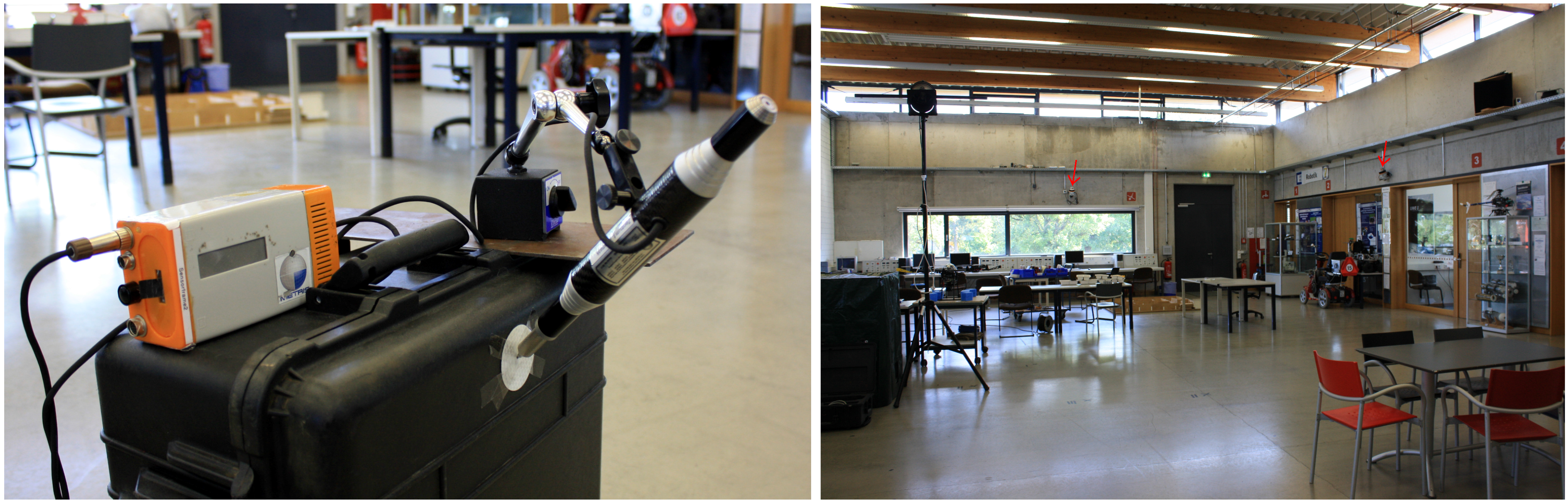
To evaluate the accuracy of our semi-rigid optimization algorithm, we acquired datasets in the robotics hall at the Julius Maximilian University of Würzburg, Germany where the iSpace system is fixed to the wall. The hall is an open space of m with desks and laboratory equipment.
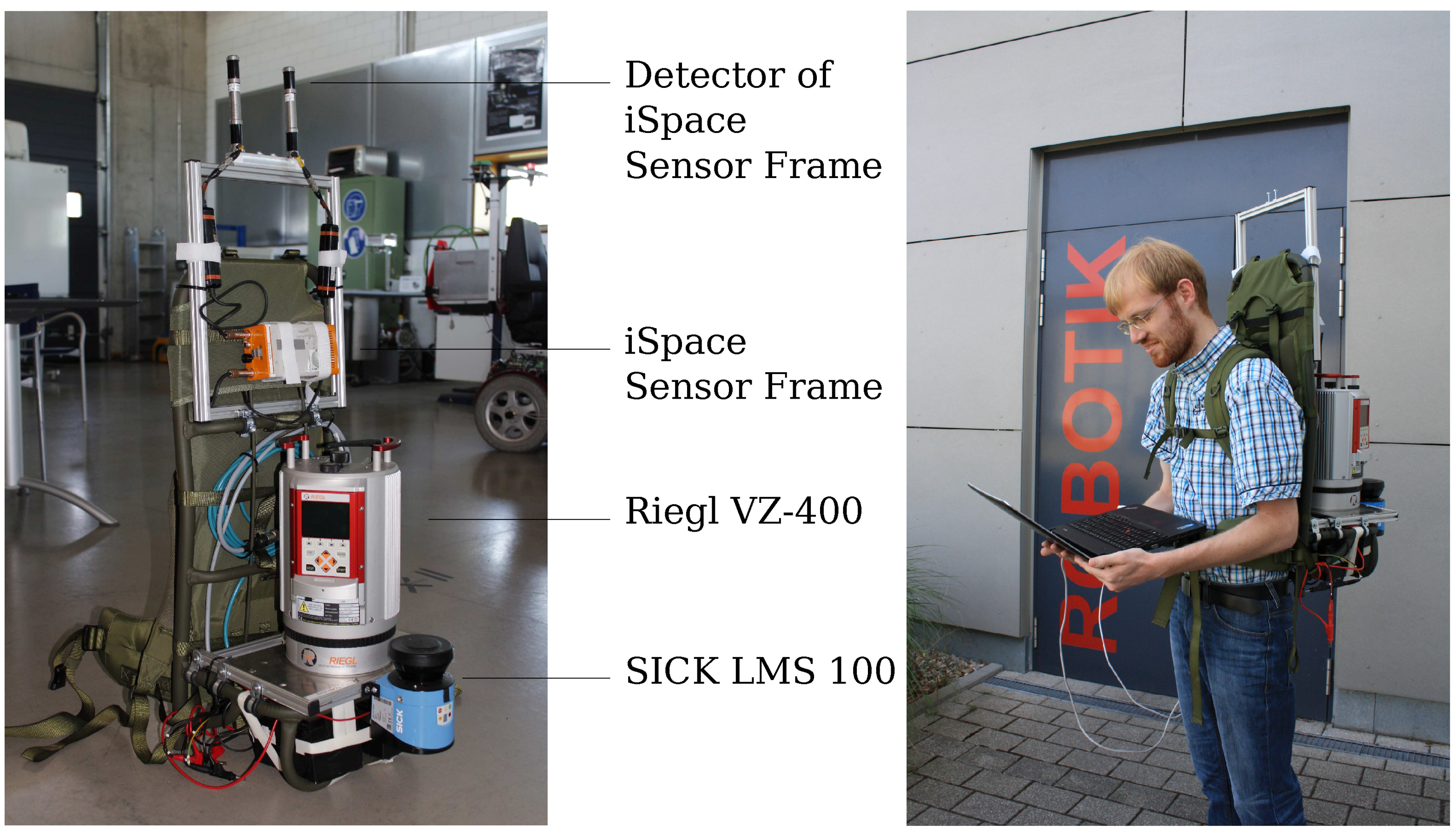
After calibrating the Riegl VZ-400 to the iSpace coordinate system, several datasets were acquired. The backpack was carried through the robotics hall by the first author along varying trajectories. To avoid the blind spot, the Riegl VZ-400 was rotating back and forth with a resolution of 0.5 degrees both horizontally and vertically with a rotational velocity of
Hz. The field of view of the scanner is restricted to
(horizontally) by
(vertically).
Table 1 shows some details of the datasets evaluated in this paper.
Table 1.
Properties of the indoor datasets evaluated in this paper.
Table 1.
Properties of the indoor datasets evaluated in this paper.
| Experiment | Shape of Trajectory | Line Scans | Duration (s) | Total Points |
|---|
| 1 | Eight | 9525 | 93 | 5,078,759 |
| 2 | Rectangle | 10,633 | 103 | 7,654,005 |
| 3 | Circle | 6201 | 60 | 4,469,067 |
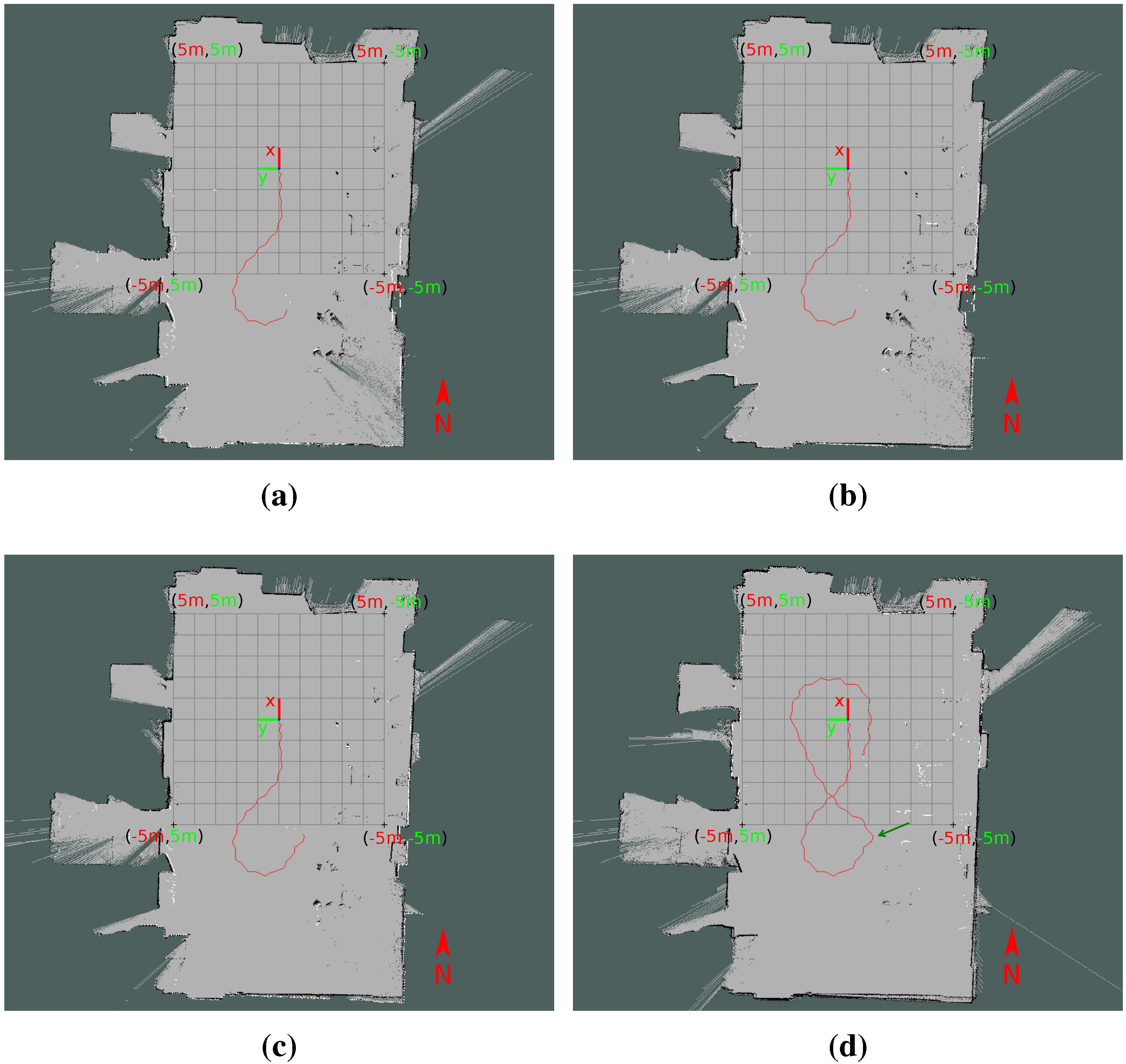
The result of the initial trajectory estimation by HectorSLAM is given in
Figure 4 and
Figure 5. While the 2D maps for Experiments 2 and 3 are consistent maps, the map for Experiment 1 shows inaccuracies on the upper end (
Figure 4). They originate from jittering in the beginning of the experiment before starting to walk. Nevertheless, the motion of normal human walking is compensated well. Difficulties arise with irregular jittering.
Figure 4 shows also inaccuracies at the lower right corner of the hall, which arise between Second 40 and Second 43 of the walk. They originate from the sharp curve in the trajectory on the right. The registration process was further affect by people walking around in this area.
Despite the small inaccuracies, the map suffices to serve as input for unwinding the Riegl data, yielding an initial 3D point cloud.
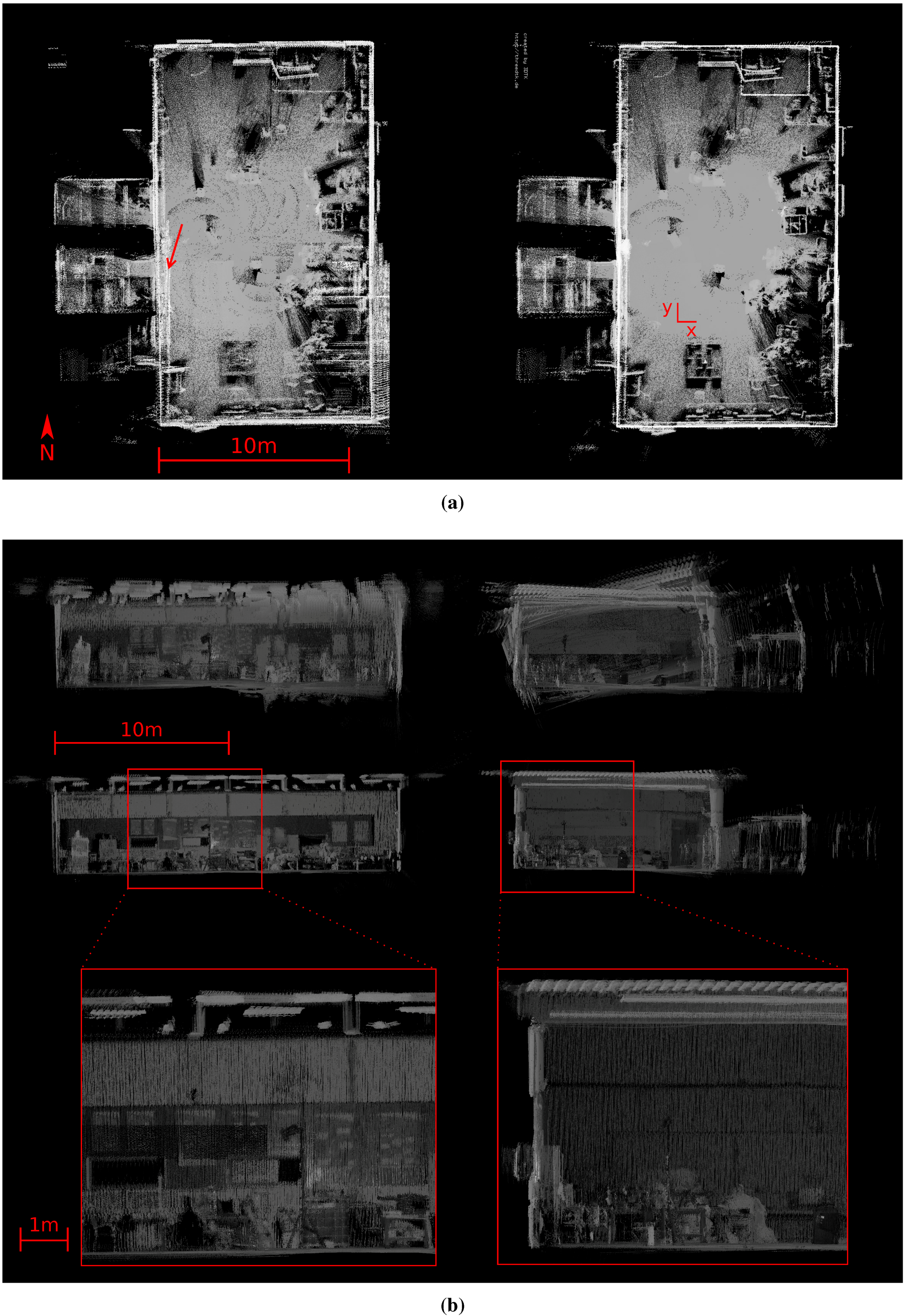
Figure 6 compares the point cloud of Experiment 1 from the bird’s eye view and two side views before and after the optimization. The quality of the point cloud improves, which is particularly evident at the walls and the floor. The gaps in the walls marked by the red arrows are closed during the optimization step.
Figure 4.
Four frames showing the 2D maps created by HectorSLAM for Experiment 1 in the local coordinate system after 41 seconds (a), 43 seconds (b), 45 seconds (c) and the final result after 93 seconds (d). The red lines denote the trajectory. The superimposed grid has a size of m. The green arrow denotes the part of the trajectory where the 2D registration lead to inaccuracies in the lower right corner between (b,c).
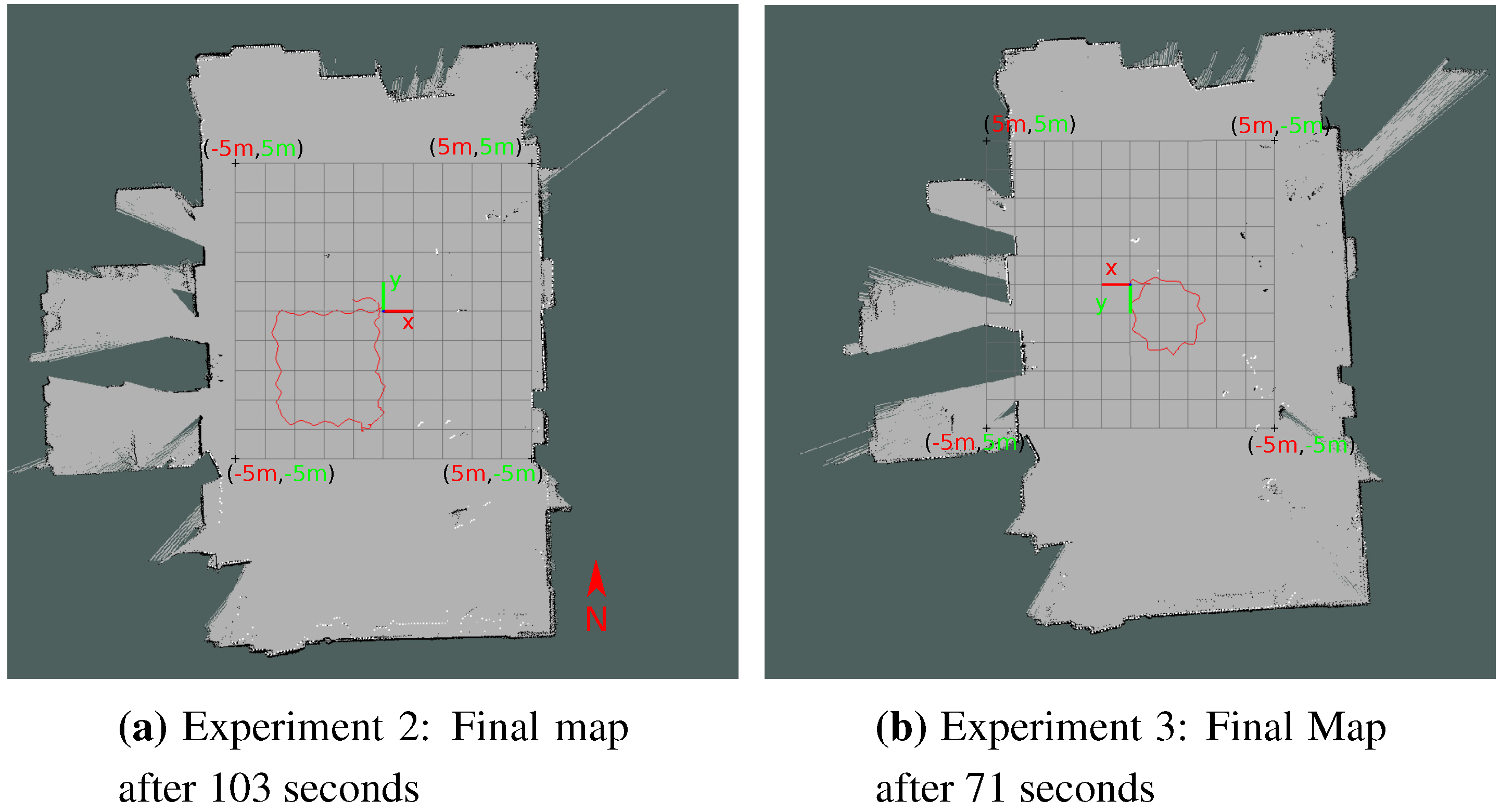
Figure 5.
Final 2D maps in the local coordinate system created by HectorSLAM for Experiments 2 (a) and 3 (b). The maps are consistent and thus serve as input for unwinding the Riegl data.
Figure 5.
Final 2D maps in the local coordinate system created by HectorSLAM for Experiments 2 (a) and 3 (b). The maps are consistent and thus serve as input for unwinding the Riegl data.
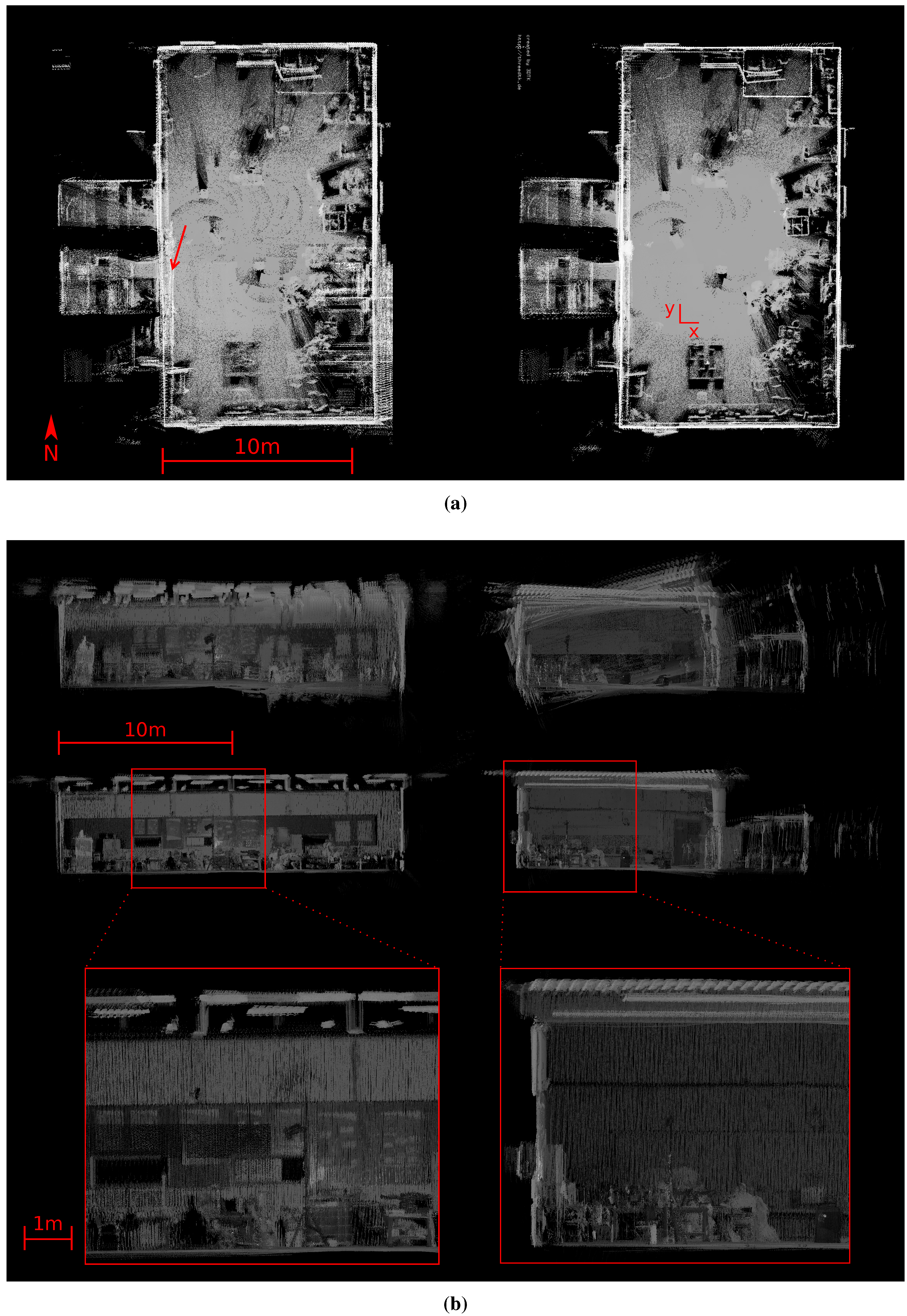
Figure 6.
3D point cloud of Experiment 1. (a) Bird’s eye view before (left) and after optimization (right). The gaps between the walls (red arrows) are closed by optimization. Depicted is the origin of the iSpace coordinate system; (b) Side view with reflectance values before (top) and after optimization (bottom). The quality improved, but the marked areas remain slightly rotated.
The remaining inaccuracies correspond to the aforementioned inaccuracies of the HectorSLAM output. Irregular jittering during the data acquisition leads to trajectory errors between neighboring line scans, which are treated as one sub-scan in the semi-rigid optimization algorithm. Thus, the error cannot be corrected completely. The marked areas in
Figure 6 result from such trajectory errors. For instance, the office door is rotated clockwise compared to the office doors outside the marked area.
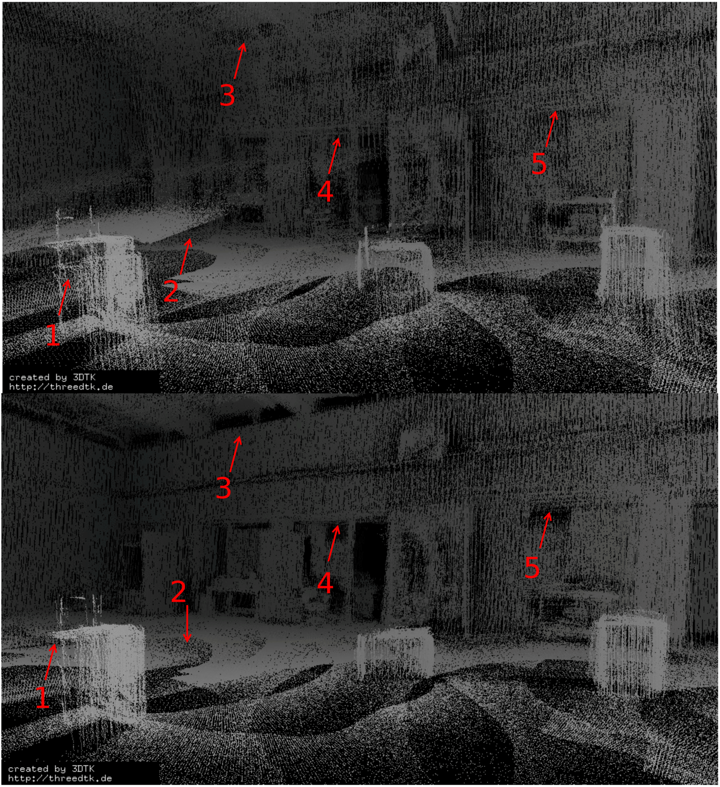
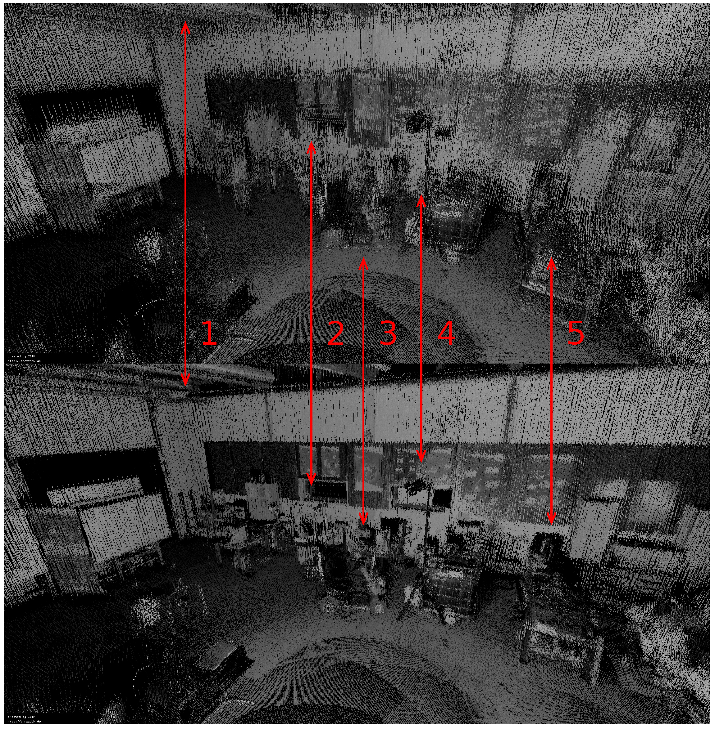
Figure 7 compares the optimization of this marked area from another perspective. While the rotated floor (Arrow 2) and the boxes (Arrow 1) converge and the windows at the ceiling (Arrow 3) become visible, the marked office doors (Arrows 4 and 5) remain rotated. In general, the structure of the environment improves, but the contours of objects are still blurry after optimization, as
Figure 8 depicts.
Figure 7.
3D point cloud of Experiment 1 without reflectance values. The color denotes the height. The boxes (1) and the rotated floor (2) converge, the windows at the ceiling (3) become visible. However, the office doors (4 and 5) remain rotated.
Figure 7.
3D point cloud of Experiment 1 without reflectance values. The color denotes the height. The boxes (1) and the rotated floor (2) converge, the windows at the ceiling (3) become visible. However, the office doors (4 and 5) remain rotated.
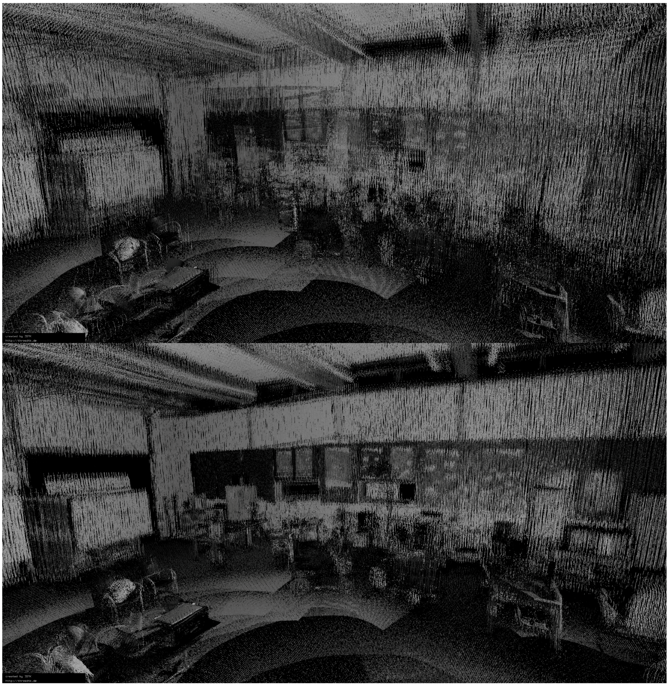
Figure 8.
3D point cloud of Experiment 1 with reflectance values. The quality improves, but the contours are still not sharp after optimization.
Figure 8.
3D point cloud of Experiment 1 with reflectance values. The quality improves, but the contours are still not sharp after optimization.
The higher quality of the initial 2D map is also reflected in the results of Experiments 2 and 3. In both experiments, the quality of the floor and the walls improve as
Figure 9 and
Figure 10 depict. Only a few line scans remain slightly rotated. In Experiment 2 a large rotational error is eliminated, as visible in
Figure 9. For Experiment 3, the main improvements appear at the floor and the ceiling.
The red arrows in
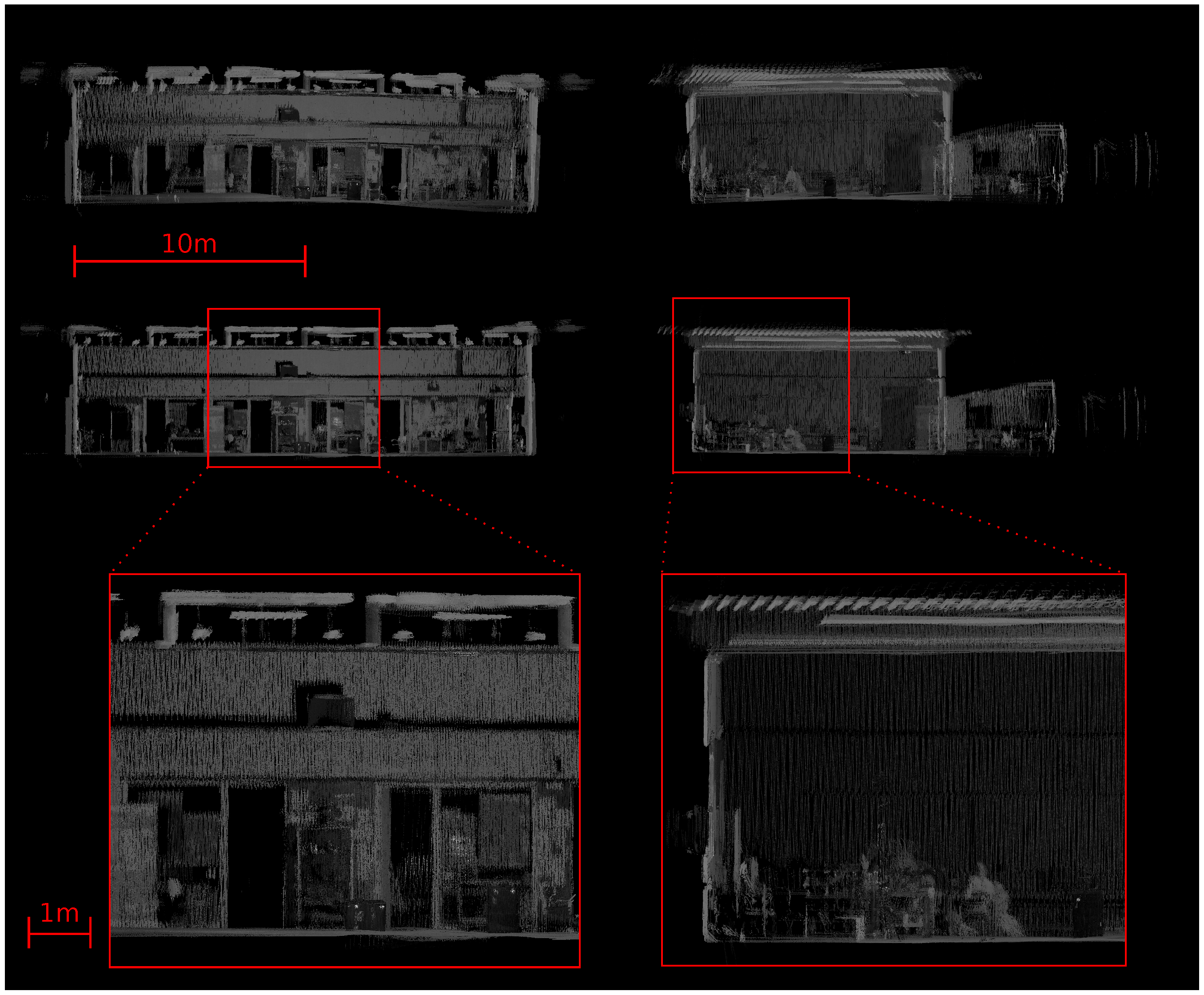
Figure 11 mark some examples where improvements from the semi-rigid optimization are clearly visible in the 3D point cloud. Sharp edges emerge, and details become distinguishable, for instance the structure of the ceiling (Arrow 1) or the objects on the table on the right (Arrow 5) (
Figure 11). Objects that appeared twice are converged successfully, e.g., the stand of the lamp (Arrow 4 in
Figure 11). Both resulting point clouds represent the environment well. The changes in
Figure 12 are not as noticeable, because the errors in the original point cloud directly after unwinding were already small.
In addition to the visual inspection, the accuracy of the backpack mobile mapping system is evaluated quantitatively using the ground truth information from the iSpace positioning system. The generated trajectories in the local coordinate system of the backpack are compared to the ground truth trajectories from the iSpace system as described in
Section 4.4.2.
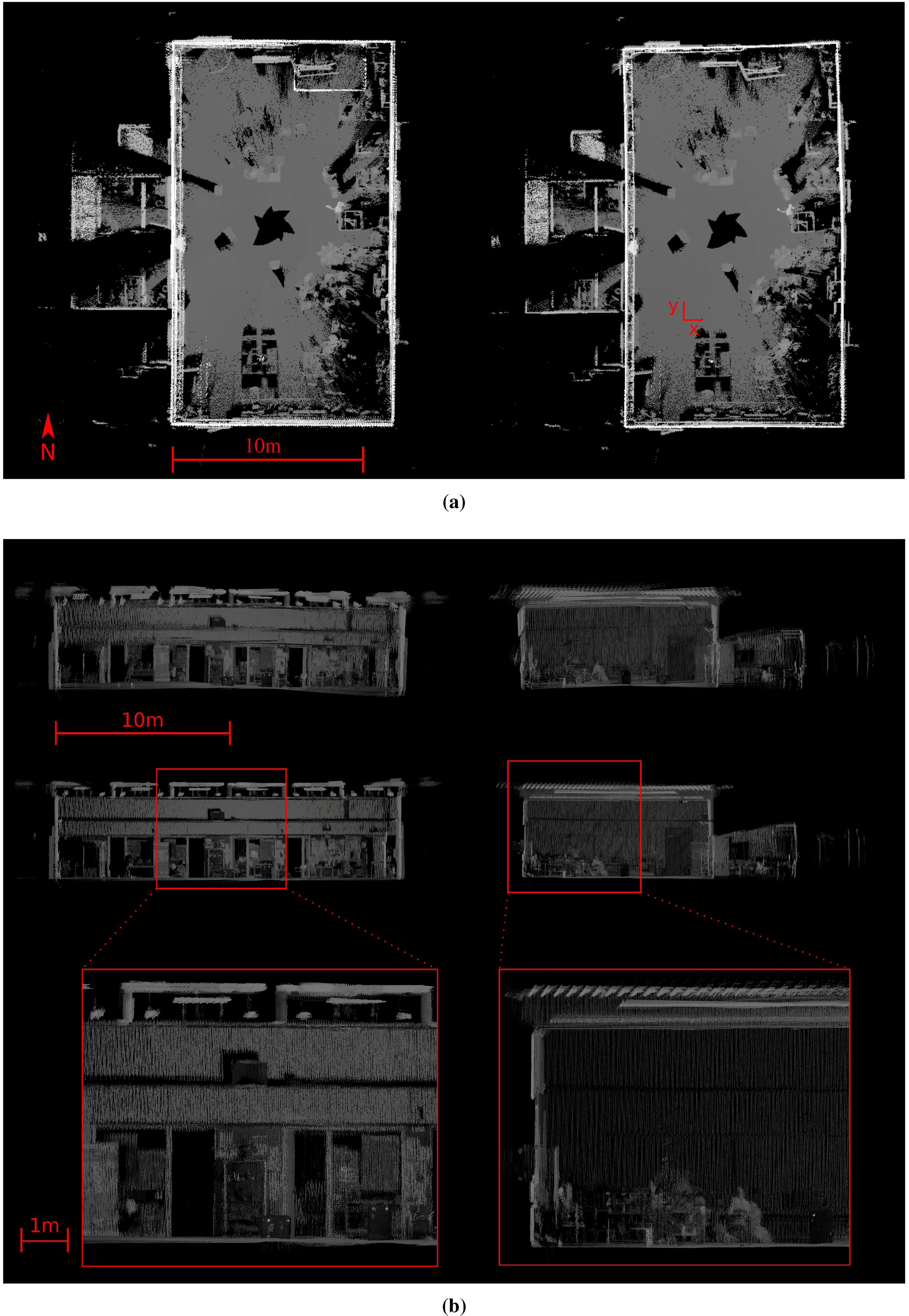
Figure 9.
3D point cloud of Experiment 2. (a) Bird’s eye view. The thickness of the walls decreased by optimization (red arrow). Depicted is the origin of the iSpace coordinate system. (b) Side views before (top) and after optimization (bottom). The scans are rotated by semi-rigid registration, such that the floor matches.
Figure 10.
3D point cloud of Experiment 3. (a) Bird’s eye view. The thickness of the walls decreased by optimization. Depicted is the origin of the iSpace coordinate system; (b) Side view before (top) and after (bottom) optimization.
Figure 10.
3D point cloud of Experiment 3. (a) Bird’s eye view. The thickness of the walls decreased by optimization. Depicted is the origin of the iSpace coordinate system; (b) Side view before (top) and after (bottom) optimization.
Figure 11.
Details from the 3D point cloud of Experiment 2. The arrows mark some examples for the improvements by semi-rigid registration. 1: the structure of the ceiling gets clearer. 2: the edges of the windows do match. 3: the scooter appears separated from the structure behind. 4: the tripod of the lamp appearing twice converged. 5: the objects on the table are distinguishable.
Figure 12.
3D view of Experiment 3 with trajectory. The structure of the scene improves, e.g., at the ceiling.
Figure 12.
3D view of Experiment 3 with trajectory. The structure of the scene improves, e.g., at the ceiling.
The resulting position and orientation errors for each experiment are given in
Table 2. For all three experiments, the error after applying the semi-rigid optimization is noted. Additionally, for comparison, the error before optimization is noted for Experiment 2. The visualization of the position and orientation errors in axis angle representation for the entire trajectories is shown in
Figure 13,
Figure 14 and
Figure 15.
Table 2.
Absolute trajectory error of the experiments. The * denotes the error before optimization.
Table 2.
Absolute trajectory error of the experiments. The * denotes the error before optimization.
| | Position Error (cm) | Orientation Error (°) |
|---|
| Exp. | RMSE | Min | Max | RMSE | Min | Max | RMSE | Min | Max |
| 1 | 11.493 | 1.807 | 23.469 | 2.960 | 0.152 | 11.039 | 2.114 | 0.00034 | 6.687 |
| 2 (*) | 6.135 | 0.232 | 29.369 | 6.685 | 0.380 | 19.927 | 2.270 | 0.00011 | 5.239 |
| 2 | 6.008 | 0.450 | 25.555 | 2.110 | 0.106 | 7.440 | 1.437 | 0.00040 | 4.495 |
| 3 | 3.405 | 0.401 | 8.520 | 1.714 | 0.033 | 4.158 | 1.335 | 0.00017 | 3.372 |
| | | Axis angle | Yaw rotation |
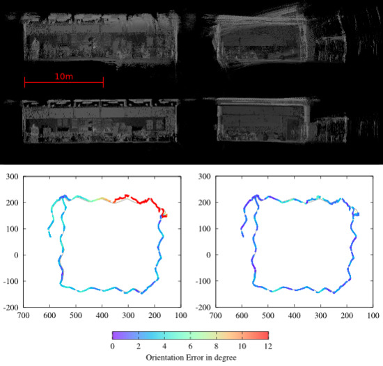
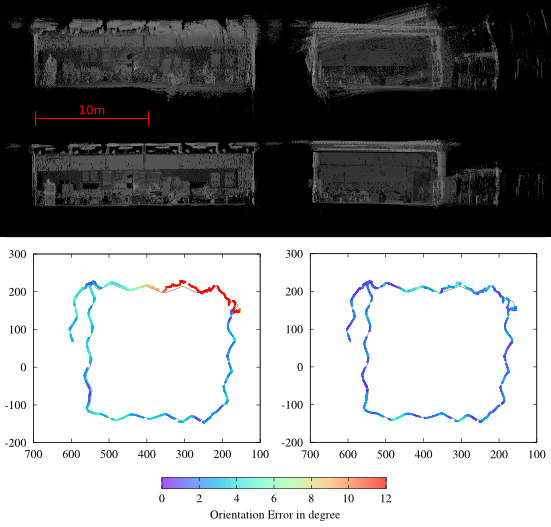
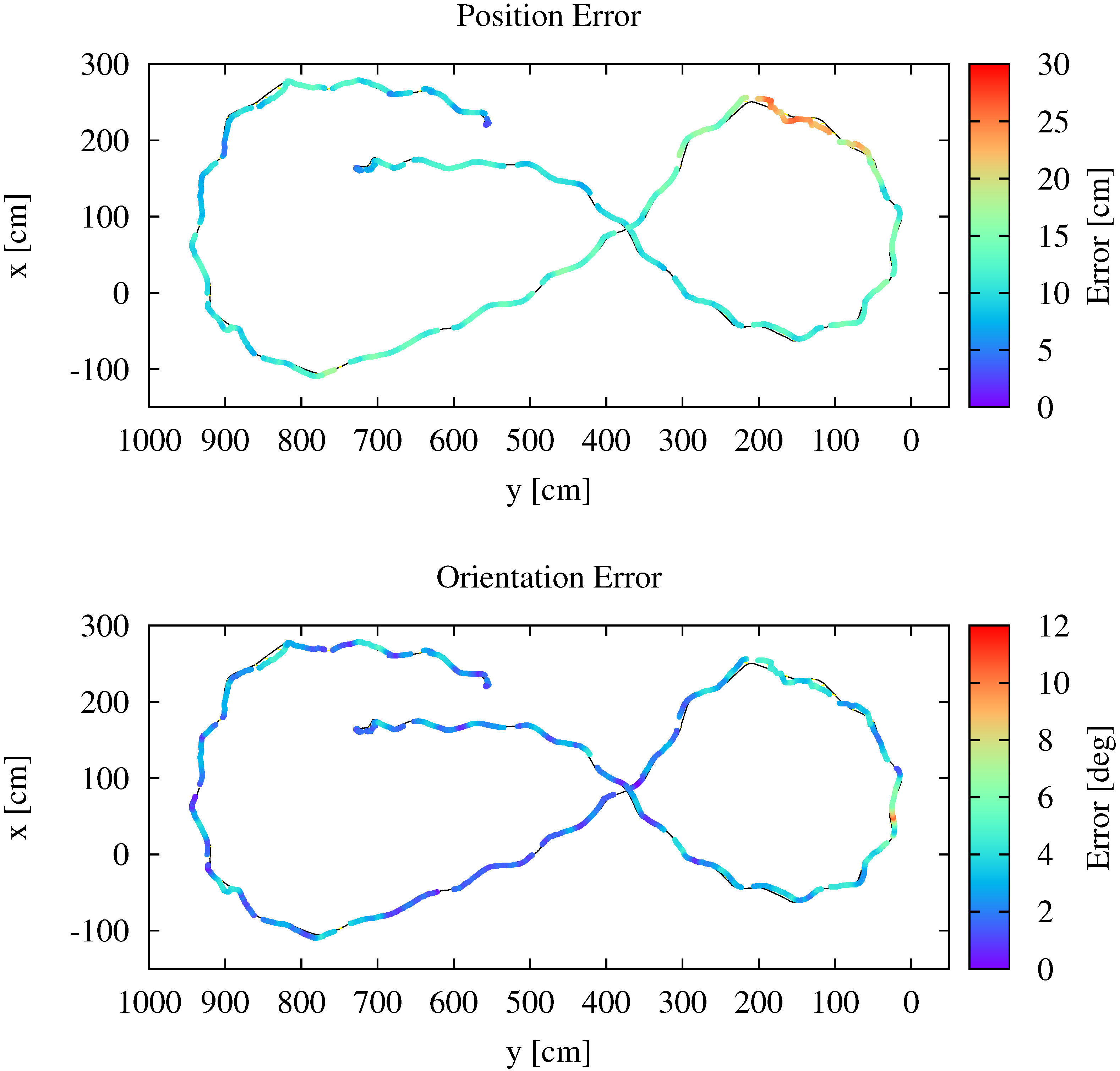
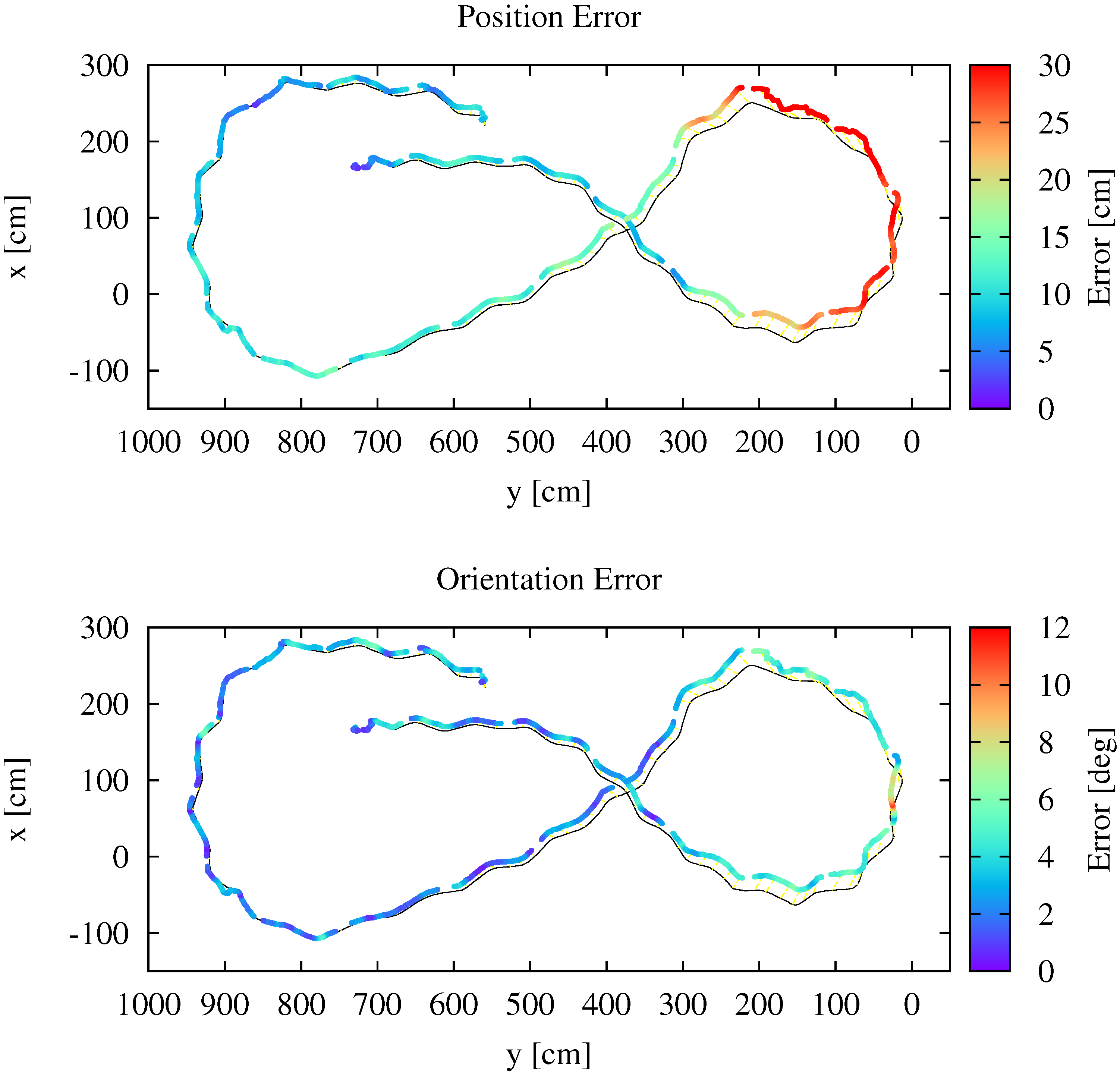
Figure 13.
Experiment 1. (Top): position error after applying semi-rigid registration. (Bottom): orientation error. The black line denotes the ground truth trajectory and the colored points the initial estimated trajectory.
Figure 13.
Experiment 1. (Top): position error after applying semi-rigid registration. (Bottom): orientation error. The black line denotes the ground truth trajectory and the colored points the initial estimated trajectory.
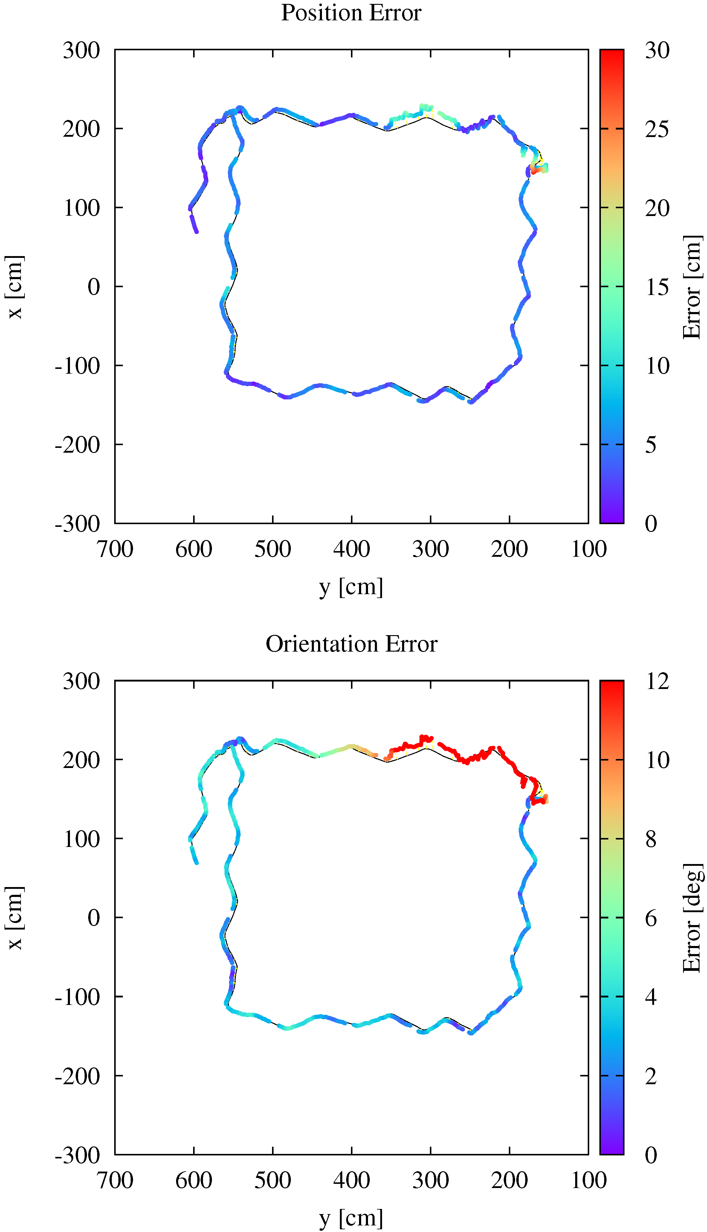
Figure 14.
Experiment 2. (Top): position error. (Bottom): orientation error.
Figure 14.
Experiment 2. (Top): position error. (Bottom): orientation error.
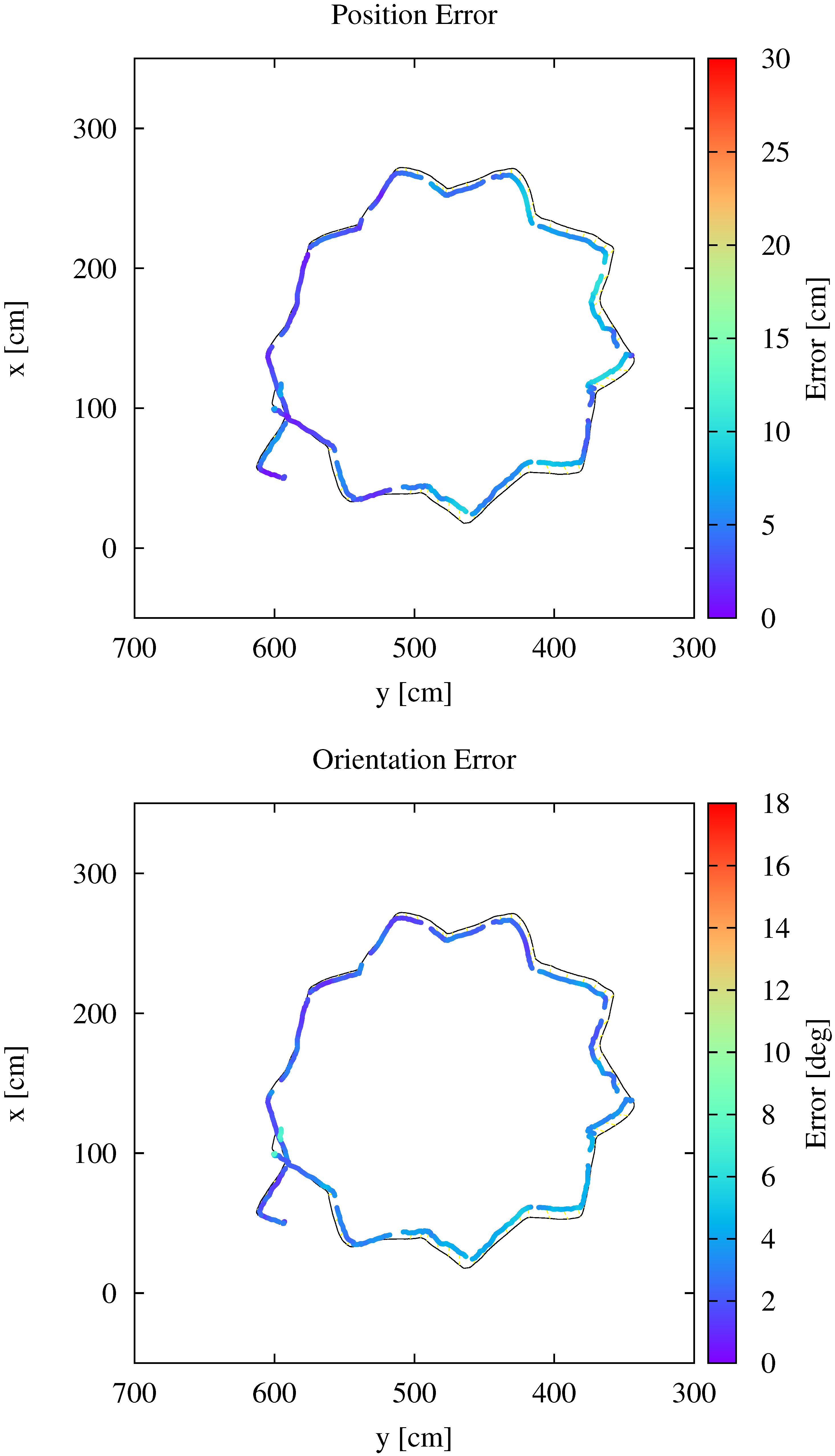
Figure 15.
Experiment 3. (Top): position error. (Bottom): orientation error.
Figure 15.
Experiment 3. (Top): position error. (Bottom): orientation error.
Figure 13 shows the error for Experiment 1. The main part of the optimized trajectory has an accuracy of 10 cm to 15 cm. Only the part in the upper left, which corresponds to the aforementioned inaccuracies in the HectorSLAM output, shows an error above 20 cm. The orientation is corrected by the semi-rigid optimization. Even in those areas where the position error remains above 20 cm, the resulting orientation error is below 6
. Only the small part on the right has an error up to 11
, which causes the rotated area marked in
Figure 6. In contrast to that,
Figure 16 gives an example for the error aligning the start poses of the trajectories for Experiment 1. Since the estimated starting pose is erroneous, the position error increases with growing distance from the starting pose up to a maximum of 41.177 cm. Therefore, this method is not evaluated further.
Figure 16.
Experiment 1. Aligning trajectories without ICP. (Top): position error after applying semi-rigid registration. (Bottom): orientation error.
Figure 16.
Experiment 1. Aligning trajectories without ICP. (Top): position error after applying semi-rigid registration. (Bottom): orientation error.
Comparing the trajectories before and after the semi-rigid optimization points out the improvements. This is shown exemplarily for Experiment 2. For Experiment 2, the inaccuracy in the position of the initially generated trajectory (
Figure 17) remains below 10 cm, except for the small part in the upper right corner where the error grows up to 29 cm. Deforming the trajectory by the optimization step even seems to increase the position error in some parts of the trajectory in order to decrease the maximum error (
Figure 14).
Table 2 points out that the optimization changes the position errors only by a few centimeters. Considering the bird’s eye view in
Figure 9, which shows that already, the initial point cloud represents the floor plan of the robotics hall well, this result can be expected. The major optimization work is done by reducing the orientation errors. They concern mainly the orientation in roll and pitch direction, as the side views in
Figure 9 visualize. The initial trajectory has an orientation error near 20
over a distance of two meters. This error is reduced such that the maximum error of the entire trajectory does not exceed 7
. Experiment 2 also demonstrates the deficits of considering only the error in yaw rotation.
Table 2 shows that the maximal orientation error in yaw rotation is 5
in contrast to the maximal error of 20
using the axis angle representation. Moreover, the errors in yaw rotation before and after optimization do not differ much, while the root mean square error is reduced to one third by considering the axis angle representation.
Figure 17.
Error for Experiment 2 before optimization. (Top): position error. (Bottom): orientation error.
Figure 17.
Error for Experiment 2 before optimization. (Top): position error. (Bottom): orientation error.
As expected from visual inspection, the position error, as well as the orientation error for Experiment 3 are small (
Figure 15). They do not exceed 9 cm in position and 4
in orientation, respectively. This experiment shows that the backpack mobile mapping system is able to produce a good point cloud representation of the environment.
5.2. Outdoor Dataset
Up to now, the backpack was only tested in indoor environments. Characteristic for those environments are optimal circumstances, like a planar ground. Moreover, the size of the scene is most often restricted; hence, all of measurements are within the range of the 2D LiDAR. In contrast to this, outdoor environments are more complex. Besides the rough terrain, large distances outside the range of the SICK scanner predominate.
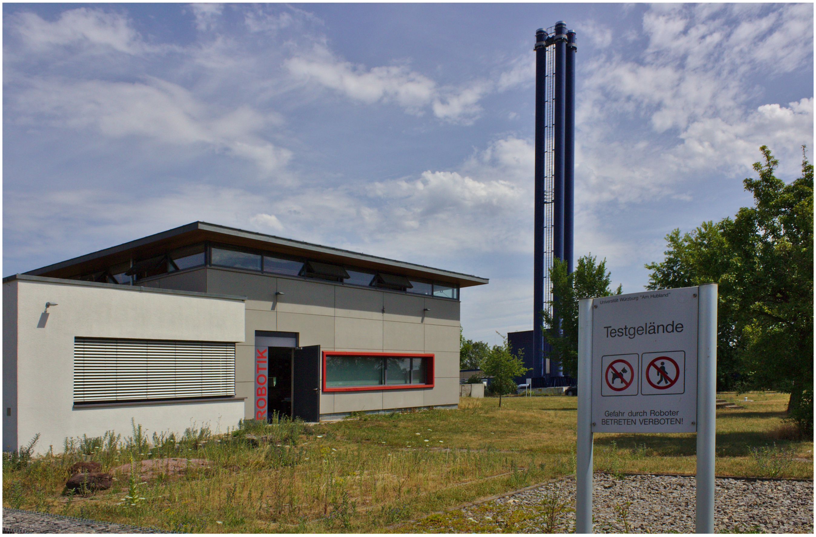
For evaluation in an urban environment, we walked a loop around the robotics hall, as depicted in
Figure 18. The outdoor robotic test area consists of challenging analog moon and mars environments, a crater, trees and plants and other structures.
Figure 19 shows part of the urban scene. The data was acquired during a walk of 276 seconds. The Riegl VZ-400 captured a total of 28,811 line scans,
i.e., 7,936,966 point measurements. The results were inspected visually.
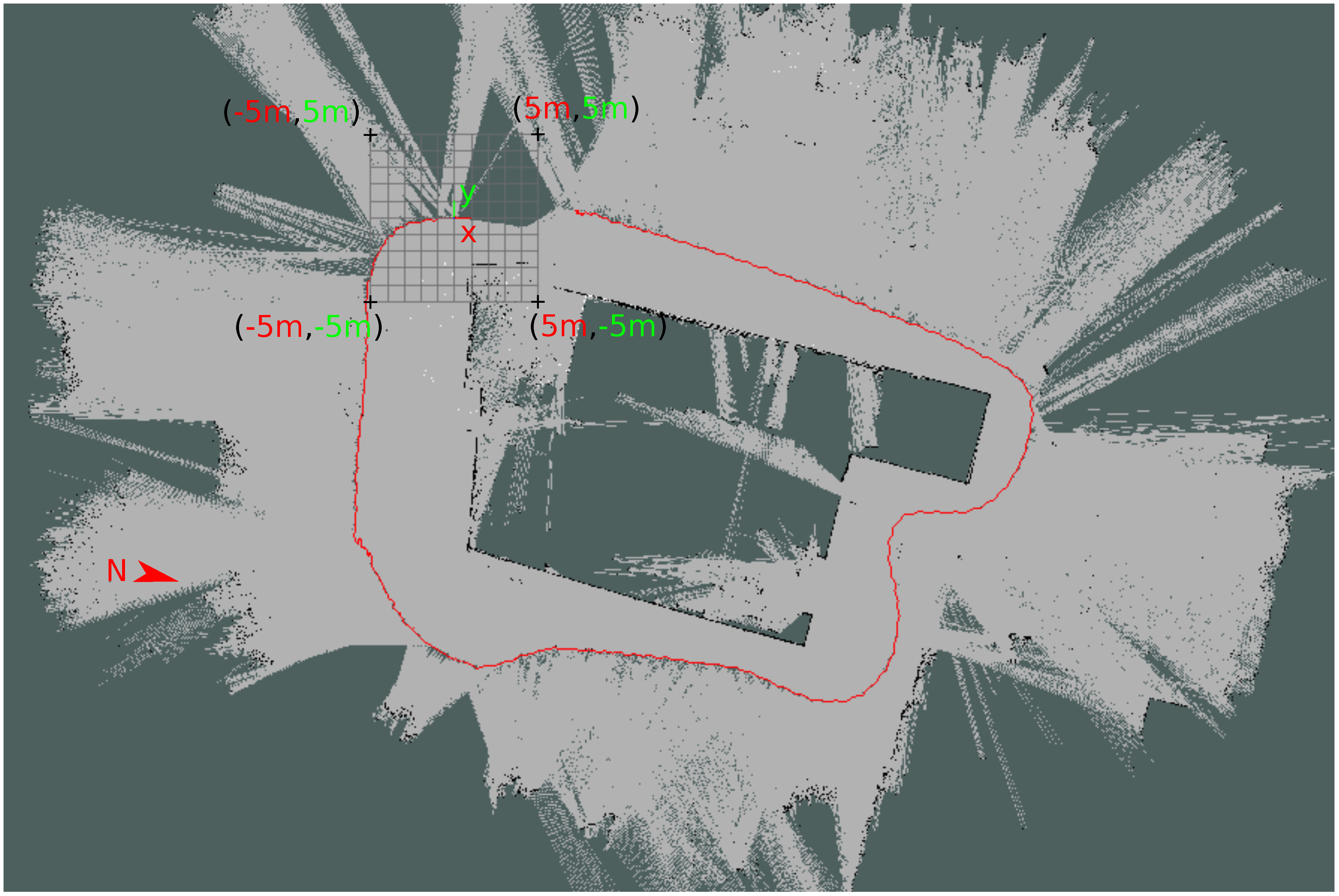
Figure 18.
2D map of the outdoor dataset created by HectorSLAM in the local coordinate system. Inaccuracies arose when the SICK scanner covered open terrain. The superimposed grid has a size of m, and the red line denotes the trajectory.
Figure 18.
2D map of the outdoor dataset created by HectorSLAM in the local coordinate system. Inaccuracies arose when the SICK scanner covered open terrain. The superimposed grid has a size of m, and the red line denotes the trajectory.
Figure 19.
The robotics hall and the robotic test field were the experiment took place. In the foreground, the areas for simulating different planetary surfaces. In the background, the chimney of the Technischer Betrieb of the university.
Figure 19.
The robotics hall and the robotic test field were the experiment took place. In the foreground, the areas for simulating different planetary surfaces. In the background, the chimney of the Technischer Betrieb of the university.
The output of HectorSLAM is shown in
Figure 18. Predominant large distances out of the range of the SICK scanner cause inaccuracies in the 2D map. The bottom left corner was not registered correctly by HectorSLAM, because the SICK field of view covered only open terrain in this area. Furthermore, the left wall of the building appears too short. Although enough features were in range, like parked cars, the homogeneous structure of the wall led to the wrong matches.
However, aligning the 3D scans is still possible by exploiting the longer range of the Riegl VZ-400. To reduce the errors from the 2D pose estimation, we apply an additional preregistration step using a modified version of the well-known ICP algorithm. One complete rotation of the Riegl VZ-400 consisting of 540 line scans is treated as one scan. These scans are registered by ICP with a maximum point-to-point distance of 150 cm. The computed transformation is distributed over all 540 line scans before applying the semi-rigid registration step, thus reducing the initial error.
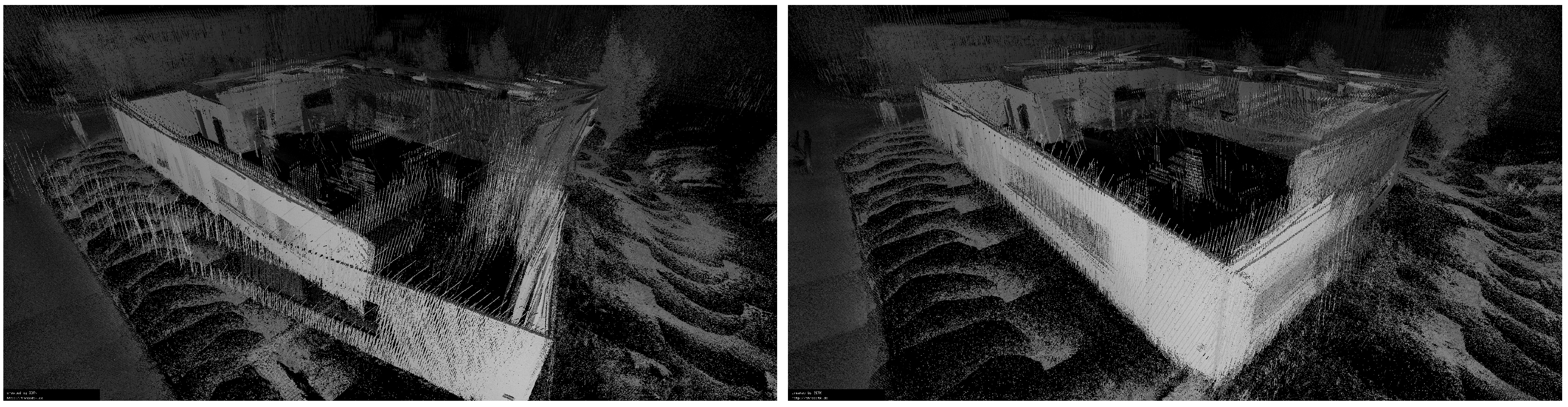
The bird’s eye view in
Figure 20 shows that the rotation error in the bottom right corner at No. 1 decreases when applying semi-rigid SLAM. Despite some inaccuracies, the walls on the left match. The parked cars at No. 3 do not appear twice anymore.
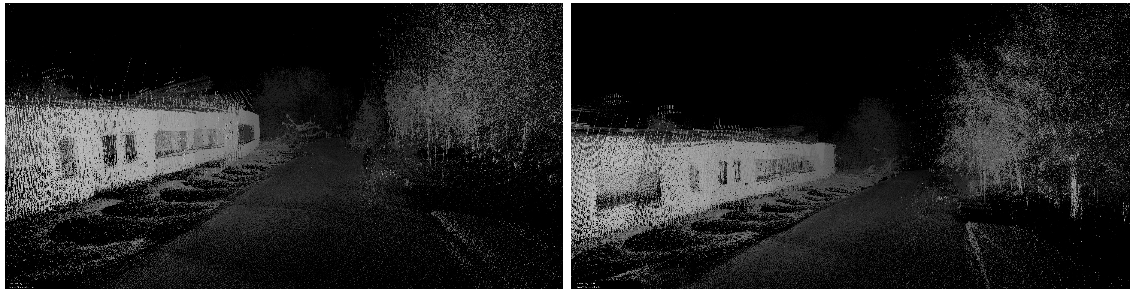
Figure 21 visualizes the optimization of the walls from another perspective. However, some inaccuracies remain after optimization. In
Figure 20, the walls at No. 2 were not matched perfectly, although the length of the wall on the left was corrected. One drawback of the preregistration step is visible at the corner of the robotics hall at No. 4. Due to the distribution of the initial transformation error over all scans, some inaccuracies increased. In general, the resulting point cloud represents the environment well.
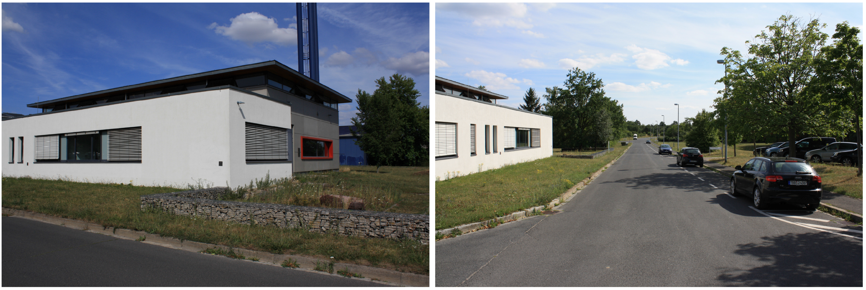
Figure 22 shows some details from the scene. In this area, even the trees appear consistent. For comparison photos of the scene are shown in
Figure 23.
Figure 20.
Bird’s eye view before (top) and after optimization (bottom). The rotation error at (1) decreased by semi-rigid optimization. The walls at (2) converged, but still do not match perfectly. The parking cars at (3) do not appear twice any more. At (4), inaccuracies increased due to distributing the initial transformation error during preregistration. The origin of the local coordinate system corresponds to the starting point of the trajectory.
Figure 21.
The walls on the left do match after optimization.
Figure 21.
The walls on the left do match after optimization.
Figure 22.
Reducing the rotation error leads to matching walls and a straight road.
Figure 22.
Reducing the rotation error leads to matching walls and a straight road.
Figure 23.
Photos showing the scene corresponding to the point clouds seen in
Figure 21 and
Figure 22.
Figure 23.
Photos showing the scene corresponding to the point clouds seen in
Figure 21 and
Figure 22.


