
Hierarchical Registration Method for Airborne and Vehicle LiDAR Point Cloud


Abstract
:
1. Introduction

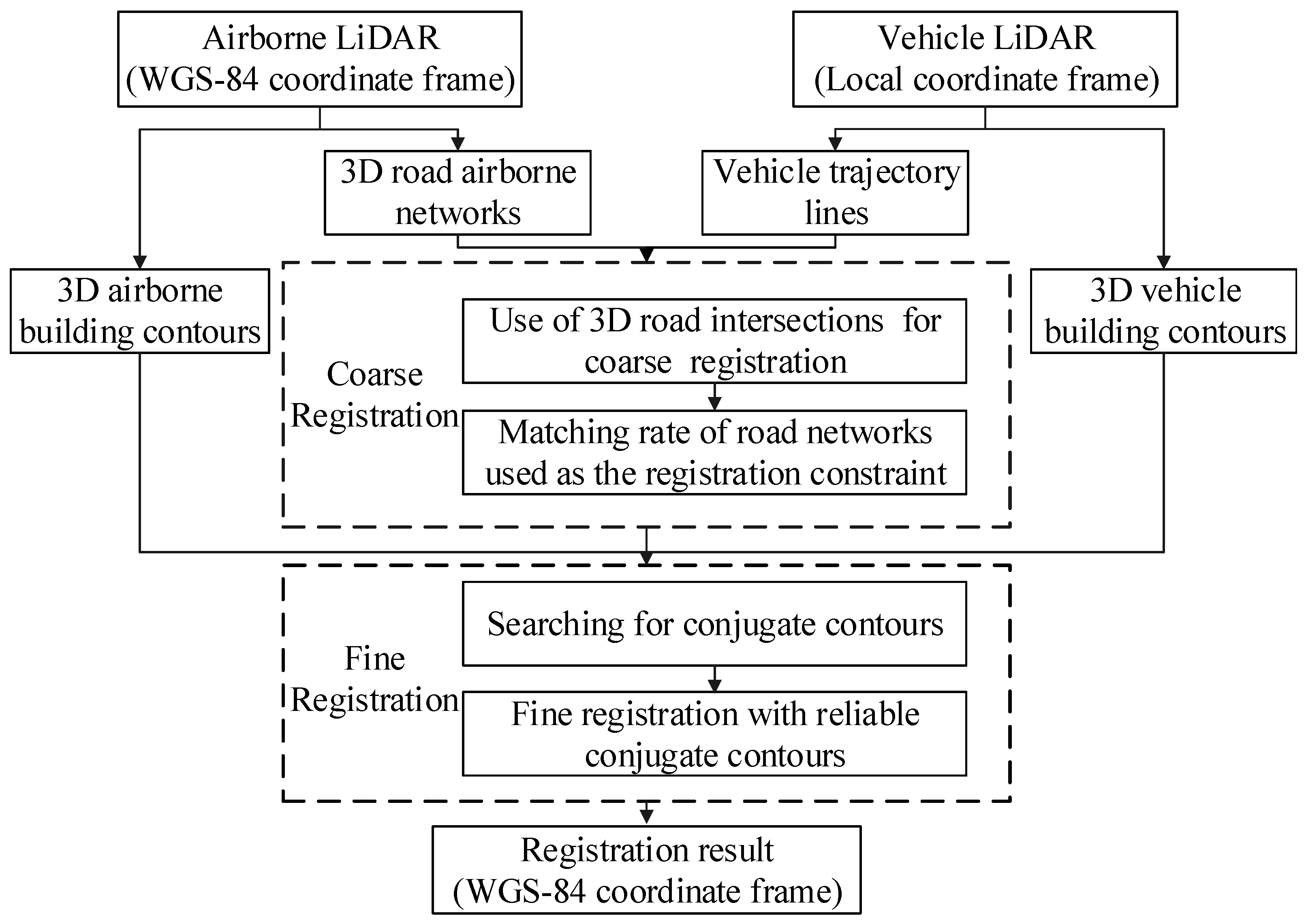
2. Method

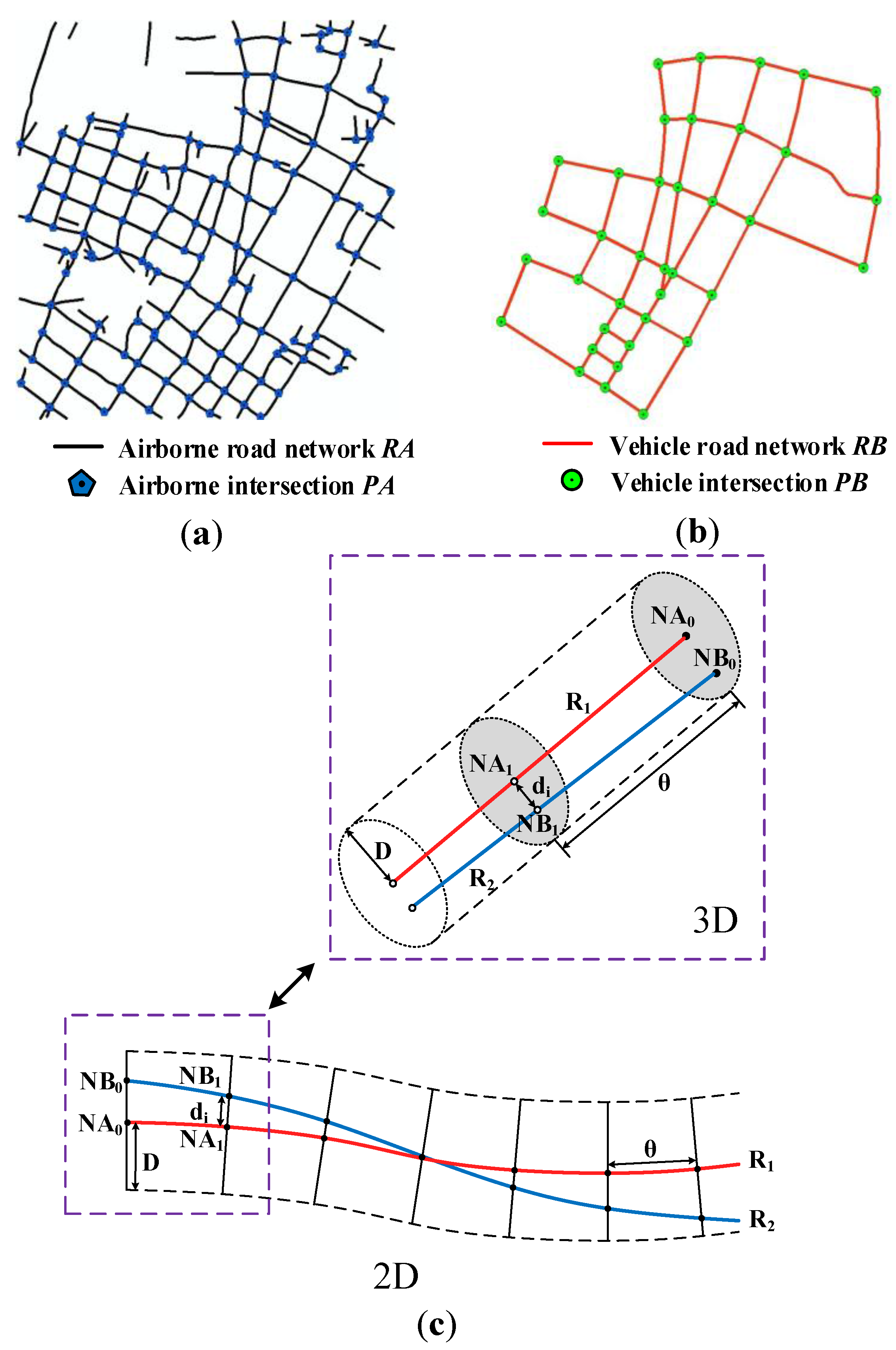
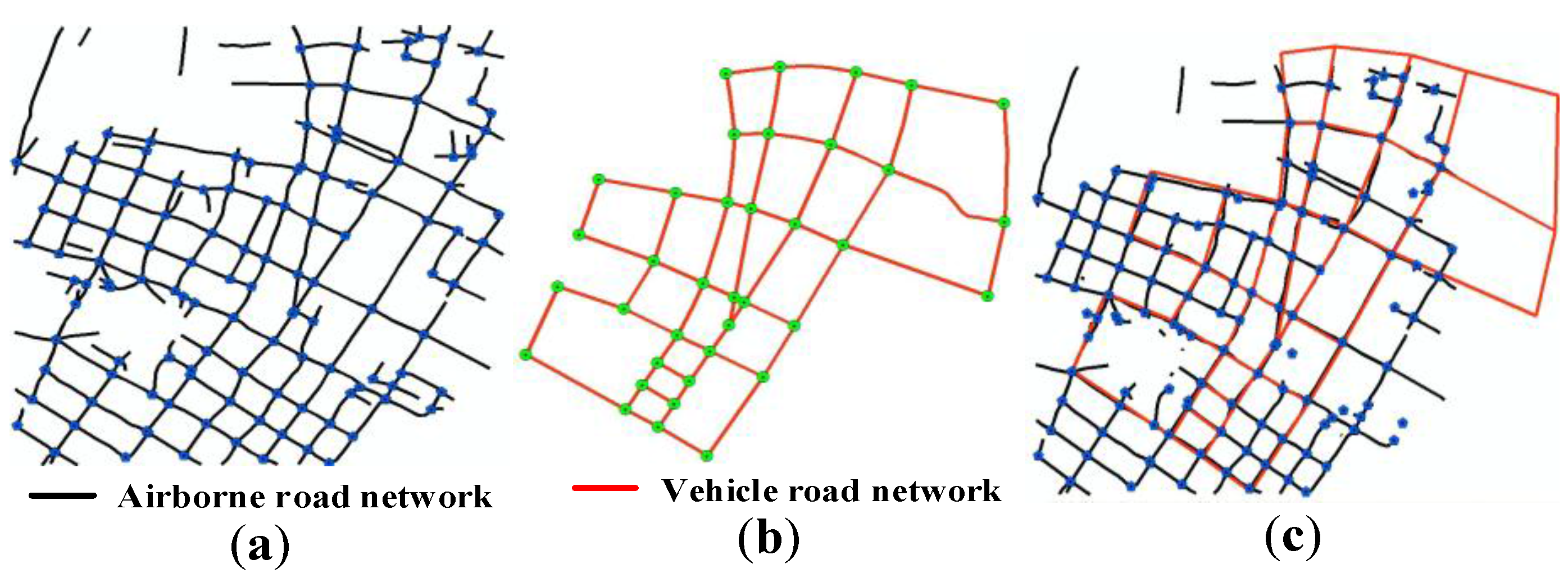
2.1. Coarse Registration with 3D Road Networks
2.1.1. 3D Road Networks from Airborne LiDAR
2.1.2. Coarse Registration with 3D Road Networks

2.2. Fine Registration with 3D Building Contours
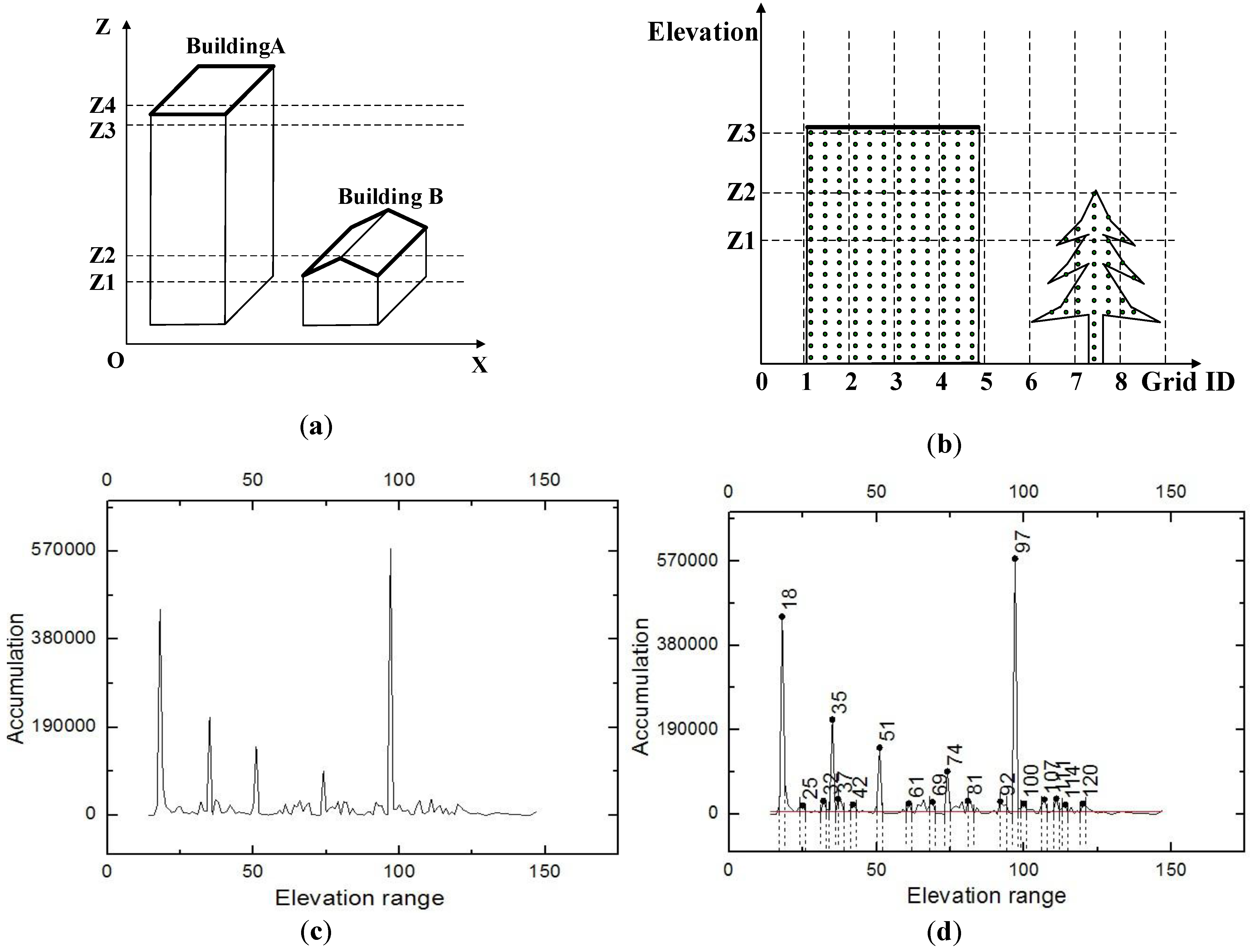
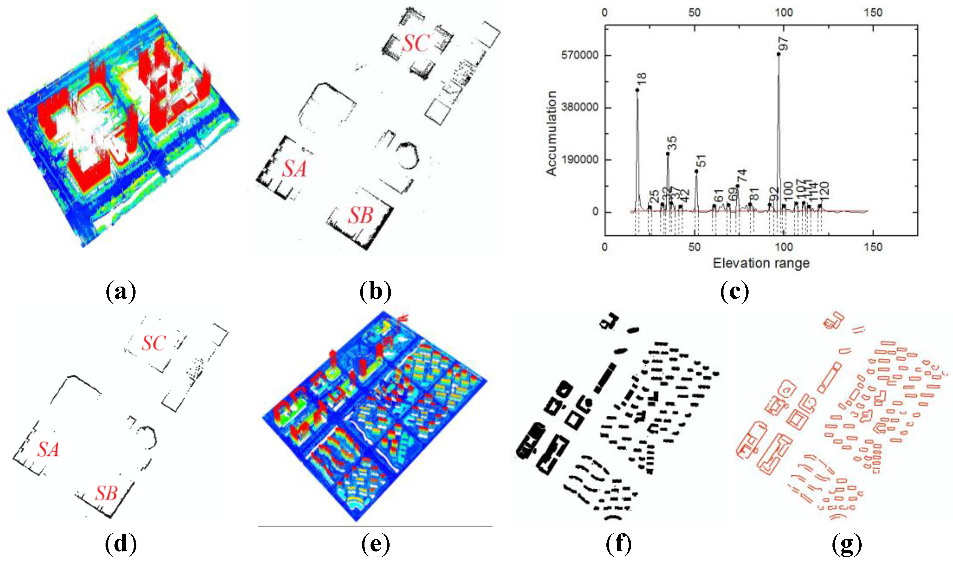
2.2.1. 2D Building Contours from Vehicle LiDAR
- (1)
- Elevation difference filtering.
- (2)
- Height value accumulation.

- (3)
- 2D contour extraction.
2.2.2. 2D Building Contours from Airborne LiDAR
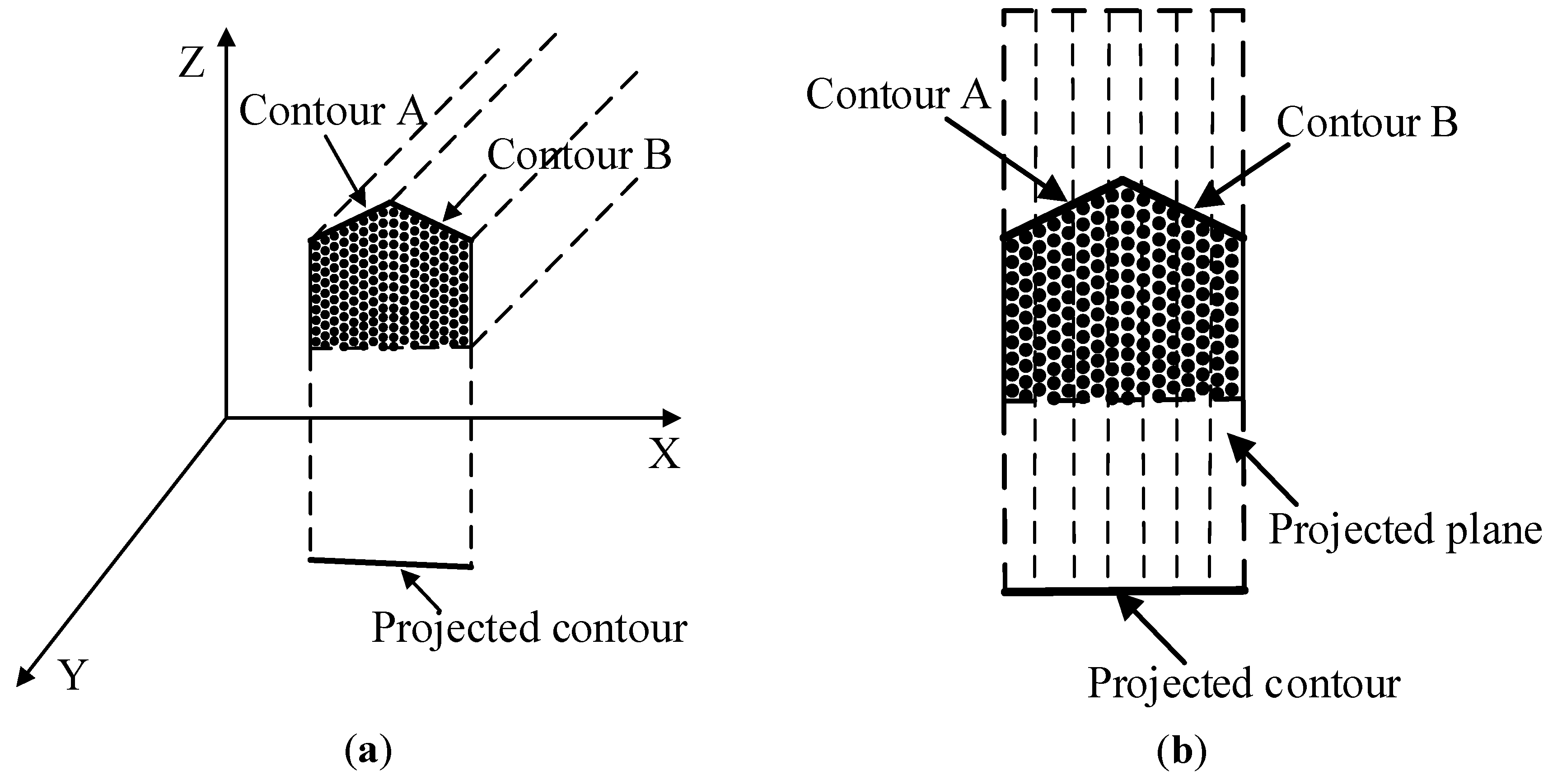
2.2.3. Extraction of 3D Building Contours
- (1)
- Projection and division of points.
- (2)
- Points clustering.
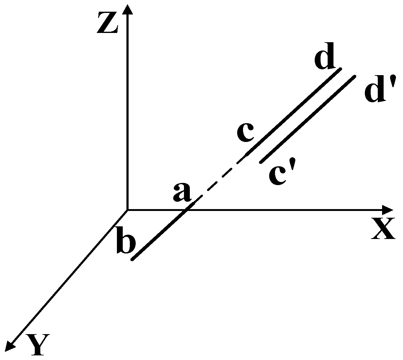
- (3)
- 3D contour fitting.

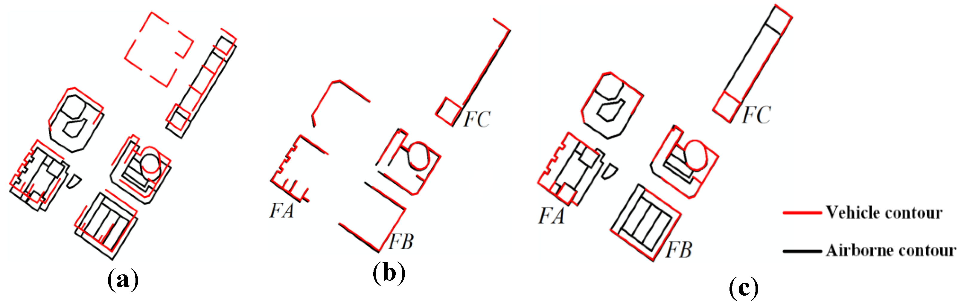
2.2.4. Fine Registration with 3D Building Contours

- (1)
- Selection of reliable conjugate contours.
- (2)
- Fine registration.
2.3. Summary of Threshold Parameters

| Method | Parameter | Scale | Setting Basis | |
|---|---|---|---|---|
| Coarse registration with road networks | Extraction of three dimensional (3D) road networks | Radius of small circle | 1 m·W/4 | Calculation |
| Determination of matching rate | Interval of 3D section planes | 1 m | Empiric | |
| The radius of section plane | 60 m | Data source | ||
| Fine registration with building contours | Extraction of two dimensional (2D) building contours from vehicle LiDAR | 2D regular grid | 1 m × 1 m | Data source |
| Elevation difference | 15 m | Data source | ||
| Elevation interval Zs | 4–5 times the average point spacing | Empiric | ||
| Extraction of 3D building contours | Elevation difference | 2 × D × I | Calculation | |
| Angle difference | 20° | Empiric | ||
| Fine registration | Angle threshold Threang | 5° | Empiric | |
| Distance threshold Thredist | 5 m (width of a lane) | Calculation | ||
| Length difference Thredif | 10 m | Empiric | ||
3. Experiments and Analysis
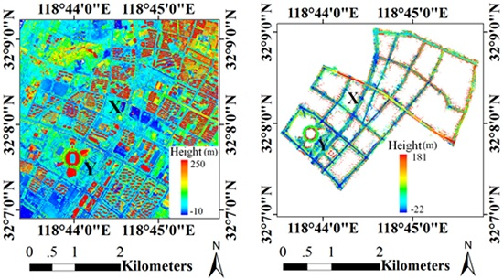
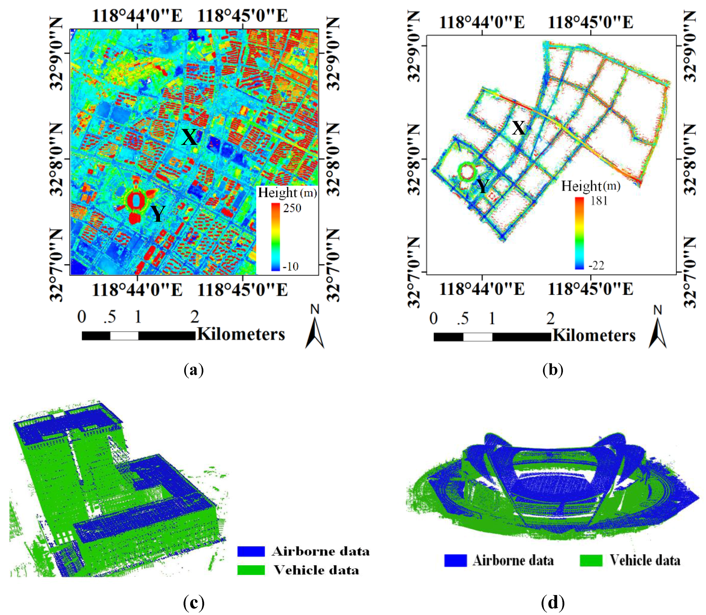
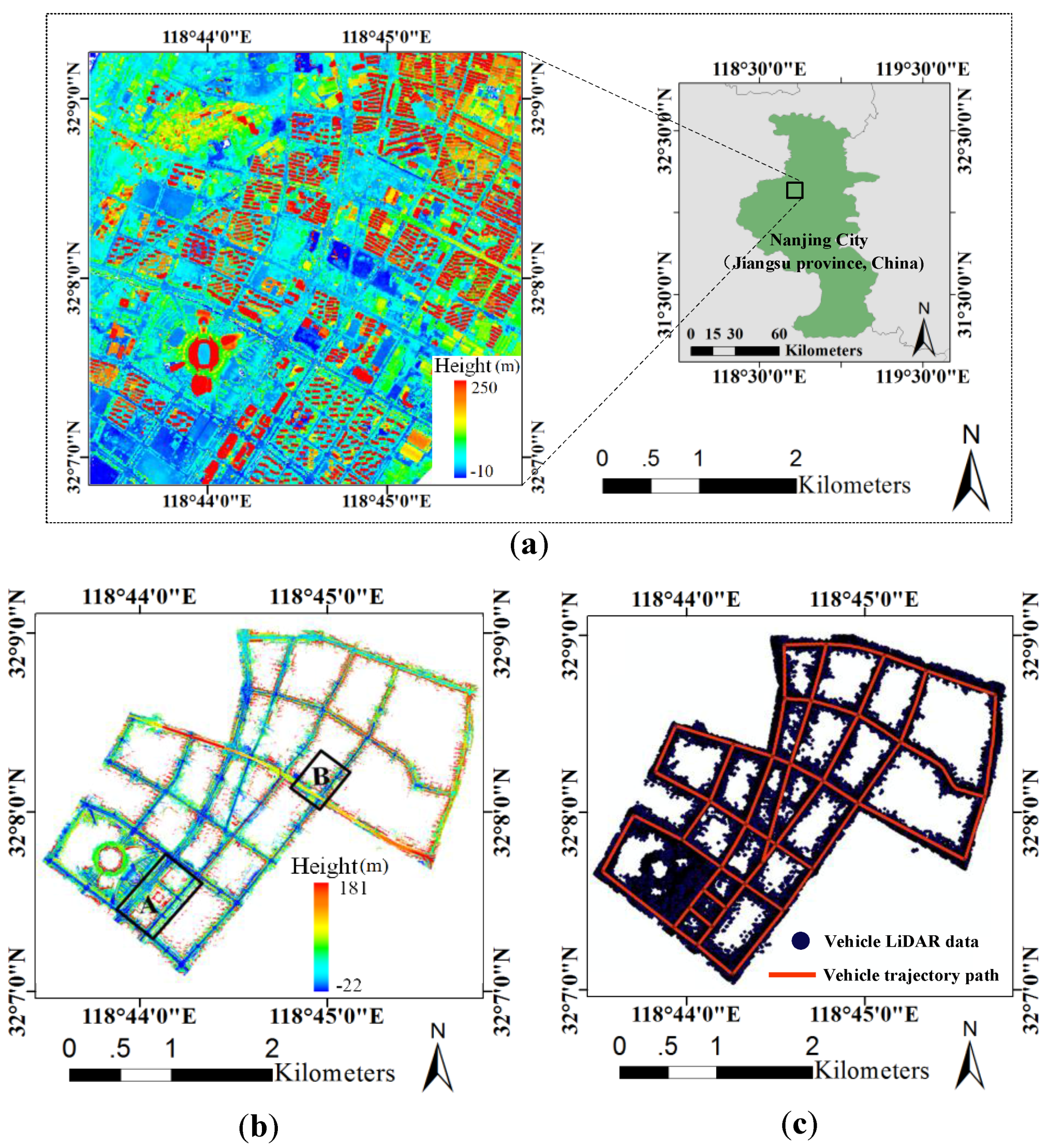
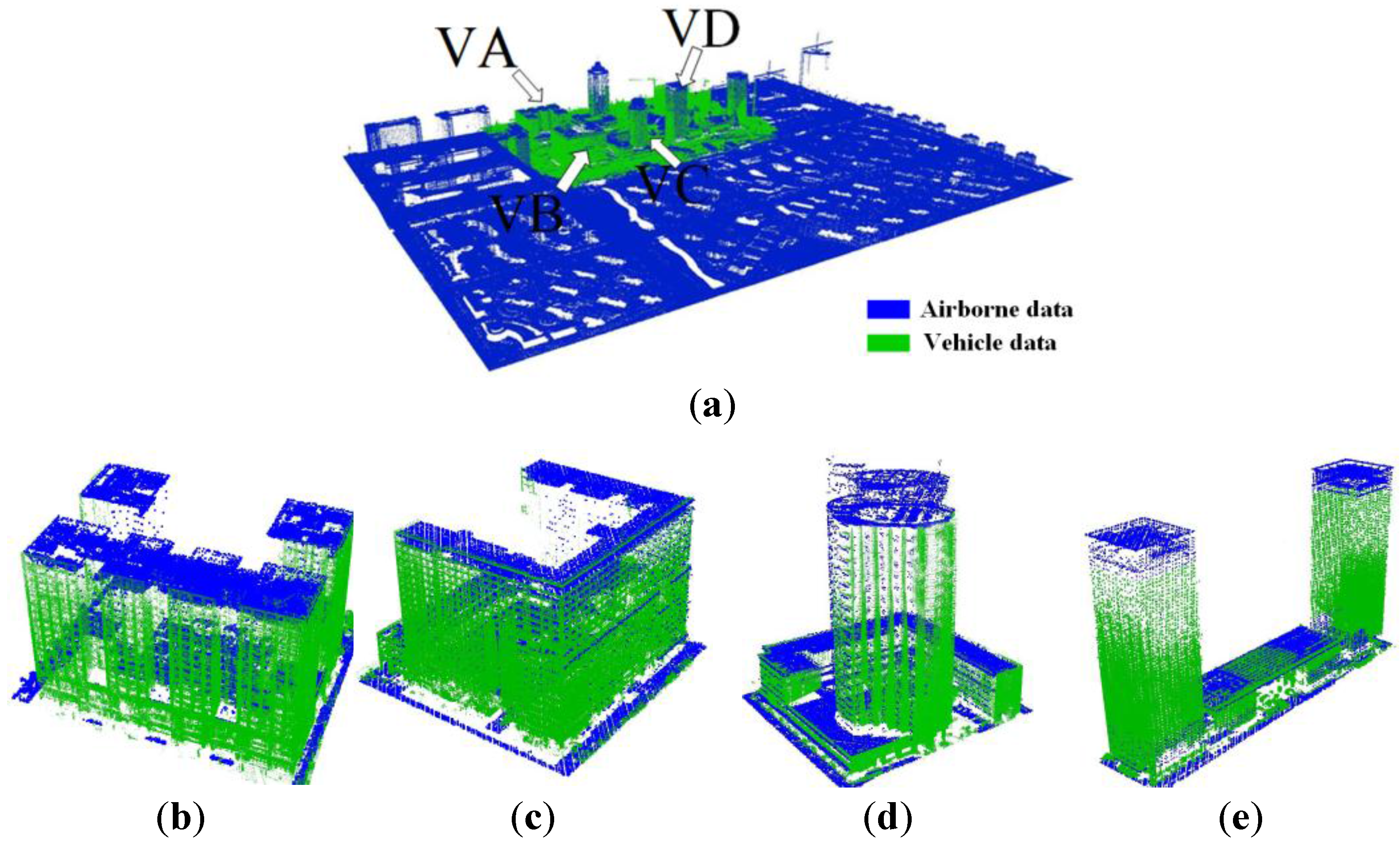
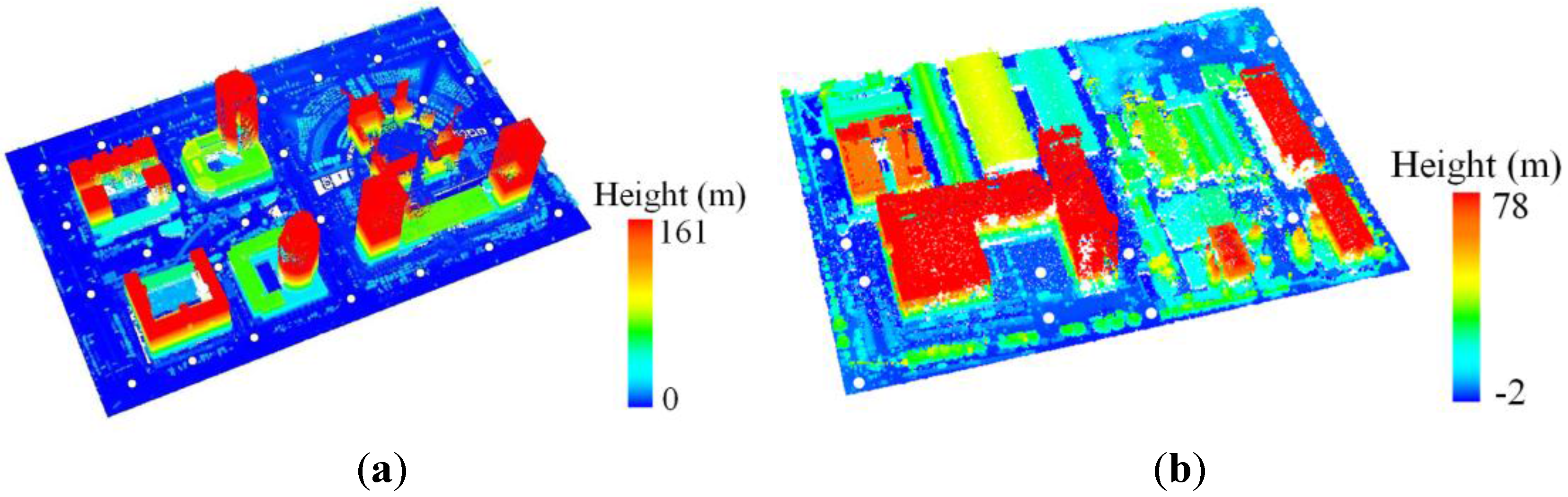
3.1. Experimental Data

3.2. Coarse Registration with 3D Road Networks

3.3. Fine Registration with 3D Building Contours
3.3.1. Extraction of 3D Building Contours

3.3.2. Fine Registration with 3D Building Contours

3.4 Result and Analysis
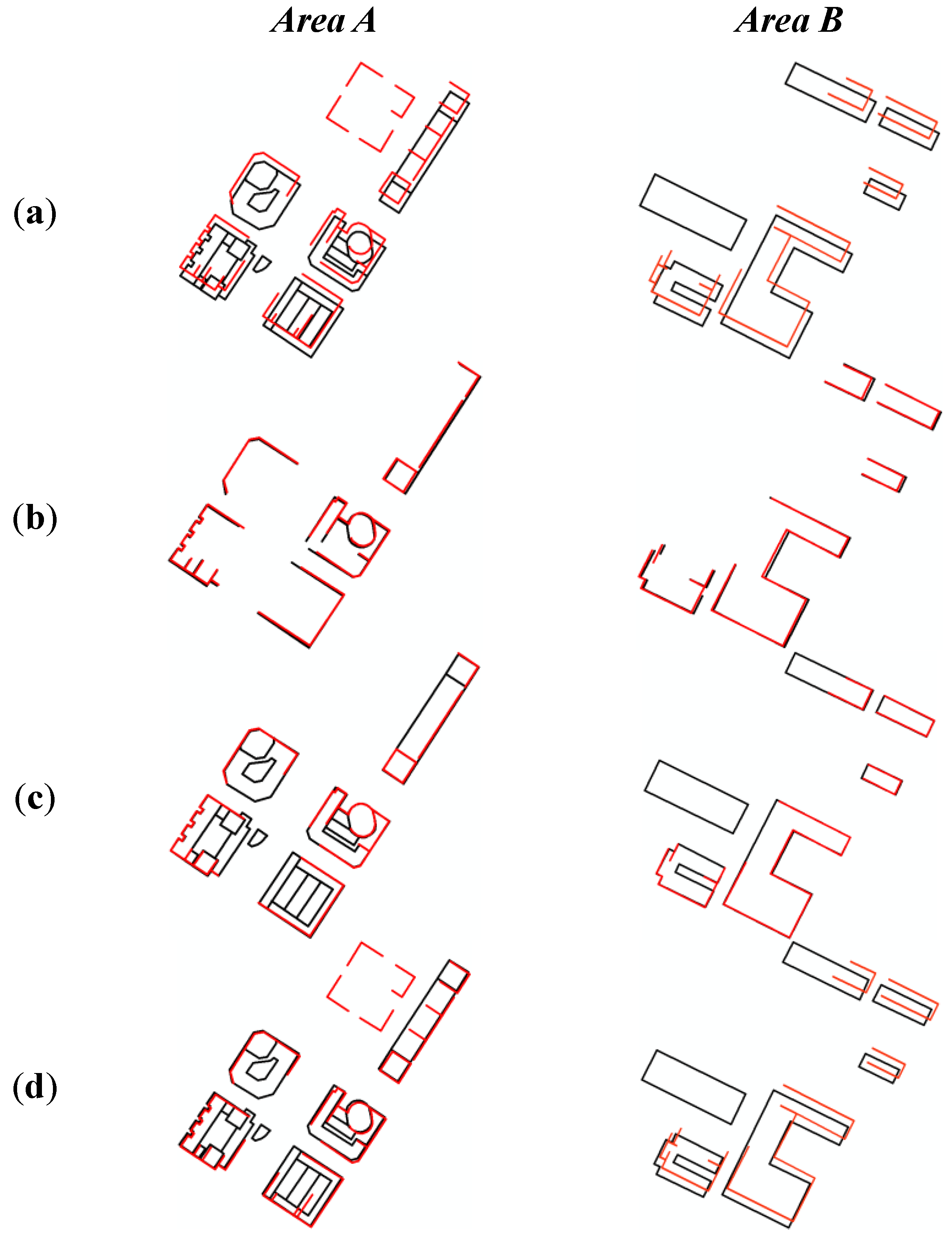
3.4.1 Visual Evaluation

3.4.2 Evaluation on Horizontal Accuracy with Building Contours

| Method | Transect Distance (m) | Line Angle (°) | |||||||||||
|---|---|---|---|---|---|---|---|---|---|---|---|---|---|
| Average | Max | Average | Max | ||||||||||
| A | B | A | B | A | B | A | B | ||||||
| Coarse registration | 17.44 | 7.43 | 21.03 | 12.68 | 0.95 | 0.88 | 1.7 | 2.1 | |||||
| Searching result | 2.53 | 1.59 | 4.30 | 3.79 | 0.82 | 0.69 | 1.6 | 1.3 | |||||
| Fine registration | 0.73 | 0.63 | 1.90 | 1.73 | 0.32 | 0.48 | 1.2 | 1.1 | |||||
| ICP refined result | 1.52 | 5.27 | 2.55 | 11.23 | 0.47 | 0.72 | 1.5 | 1.9 | |||||
3.4.3. Evaluation on Vertical Accuracy with Common Ground Points

| Method | Average Error (m) | Max Error (m) | RMSE (m) | |||
|---|---|---|---|---|---|---|
| A/B | A/B | A/B | ||||
| Coarse registration | 0.92/1.08 | 1.17/1.33 | 0.97/0.84 | |||
| Searching result | 0.46/0.59 | 0.63/0.92 | 0.50/0.68 | |||
| Fine registration | 0.39/0.43 | 0.50/0.75 | 0.42/0.36 | |||
| ICP result | 0.37/0.46 | 0.61/0.72 | 0.28/0.21 | |||
4. Discussion
5. Conclusions
Acknowledgments
Author Contributions
Conflicts of Interest
References
- Wu, B.; Yu, B.; Yue, W.; Shu, S.; Tan, W.; Hu, C.; Huang, Y.; Wu, J.; Liu, H. A voxel-based method for automated identification and morphological parameters estimation of individual street trees from mobile laser scanning data. Remote Sens. 2013, 5, 584–611. [Google Scholar] [CrossRef]
- Meng, X.; Currit, N.; Zhao, K. Ground filtering algorithms for airborne LiDAR data: A review of critical issues. Remote Sens. 2010, 2, 833–860. [Google Scholar] [CrossRef]
- Cheng, L.; Gong, J.; Li, M.; Liu, Y. 3D building model reconstruction from multi-view aerial imagery and LiDAR data. Photogramm. Eng. Remote Sens. 2011, 77, 125–139. [Google Scholar] [CrossRef]
- Cheng, L.; Wu, Y.; Wang, Y.; Zhong, L.; Chen, Y.; Li, M. Three-dimensional reconstruction of large multilayer interchange bridge using airborne LiDAR data. IEEE J. Sel. Top. Appl. Earth Obs. Remote Sens. 2014, 8, 691–707. [Google Scholar] [CrossRef]
- Kent, R.; Lindsell, J.A.; Laurin, G.V.; Valentini, R.; Coomes, D.A. Airborne LiDAR detects selectively logged tropical forest even in an advanced stage of recovery. Remote Sens. 2015, 7, 8348–8367. [Google Scholar] [CrossRef]
- Cheng, L.; Tong, L.; Wang, Y.; Li, M. Extraction of urban power lines from vehicle-borne LiDAR data. Remote Sens. 2014, 6, 3302–3320. [Google Scholar] [CrossRef]
- Lehtomäki, M.; Jaakkola, A.; Hyyppä, J.; Kukko, A.; Kaartinen, H. Detection of vertical pole-like objects in a road environment using vehicle-based laser scanning data. Remote Sens. 2010, 2, 641–664. [Google Scholar] [CrossRef]
- Yang, B.; Wei, Z.; Li, Q.; Li, J. Automated extraction of street-scene objects from mobile LiDAR point clouds. Int. J. Remote Sens. 2012, 33, 5839–5861. [Google Scholar] [CrossRef]
- Cheng, L.; Zhao, W.; Han, P.; Zhang, W.; Shan, J.; Liu, Y.; Li, M. Building region derivation from LiDAR data using a reversed iterative mathematic morphological algorithm. Opt. Commun. 2012, 286, 244–250. [Google Scholar] [CrossRef]
- Weinmann, M.; Weinmann, M.; Hinz, S.; Jutzi, B. Fast and automatic image-based registration of TLS data. ISPRS-J. Photogramm. Remote Sens. 2011, 66, S62–S70. [Google Scholar] [CrossRef]
- Böhm, J.; Haala, N. Efficient integration of aerial and terrestrial laser data for virtual city modeling using lasermaps. In Proceedings of ISPRS WG III/3, III/4, V/3 Workshop on Laser Scanning, Enschede, the Netherlands, 12–14 September 2005; pp. 12–14.
- Hohenthal, J.; Alho, P.; Hyyppä, J.; Hyyppä, H. Laser scanning applications in fluvial studies. Prog. Phys. Geogr. 2011, 35, 782–809. [Google Scholar] [CrossRef]
- Bremer, M.; Sass, O. Combining airborne and terrestrial laser scanning for quantifying erosion and deposition by a debris flow event. Geomorphology 2012, 138, 49–60. [Google Scholar] [CrossRef]
- Heckman, T.; Bimböse, M.; Krautblatter, M.; Haas, F.; Becht, M.; Morche, D. From geotechnical analysis to quantification and modelling using LiDAR data: A study on rockfall in the Reintal catchment, Bavarian Alps, Germany. Earth Surf. Process. Landf. 2012, 37, 119–133. [Google Scholar] [CrossRef]
- Besl, P.J.; McKay, N.D. A method for registration of 3-D shapes. IEEE Trans. Pattern Anal. Mach. Intell. 1992, 14, 239–256. [Google Scholar] [CrossRef]
- Chen, H.; Bhanu, B. 3D free-form object recognition in range images using local surface patches. Pattern Recognit. Lett. 2007, 28, 1252–1262. [Google Scholar] [CrossRef]
- He, B.; Lin, Z.; Li, Y.F. An automatic registration algorithm for the scattered point clouds based on the curvature feature. Opt. Laser Technol. 2012, 46, 53–60. [Google Scholar] [CrossRef]
- Makadia, A.; Patterson, A.I.; Daniilidis, K. Fully automatic registration of 3D point clouds. In Proceedings of IEEE Computer Society Conference on Computer Vision and Pattern Recognition, New York, NY, USA, 17–22 June 2006; pp. 1297–1304.
- Bae, K.; Lichti, D. A method for automated registration of unorganized point clouds. ISPRS J. Photogramm. Remote Sens. 2008, 63, 36–54. [Google Scholar] [CrossRef]
- Barnea, S.; Filin, S. Keypoint based autonomous registration of terrestrial laser point-clouds. ISPRS-J. Photogramm. Remote Sens. 2008, 63, 19–35. [Google Scholar] [CrossRef]
- Cheng, L.; Tong, L.; Li, M.; Liu, Y. Semi-automatic registration of airborne and terrestrial laser scanning data using building corner matching with boundaries as reliability check. Remote Sens. 2013, 5, 6260–6283. [Google Scholar]
- Cheng, L.; Tong, L.; Wu, Y.; Chen, Y.; Li, M. Shiftable leading point method for high accuracy registration of airborne and terrestrial LiDAR data. Remote Sens. 2015, 7, 1915–1936. [Google Scholar] [CrossRef]
- Eo, Y.D.; Pyeon, M.W.; Kim, S.W.; Kim, J.R. Coregistration of terrestrial LiDAR points by adaptive scale-invariant feature transformation with constrained geometry. Autom. Constr. 2012, 25, 49–58. [Google Scholar] [CrossRef]
- Jaw, J.J.; Chuang, T.Y. Registration of ground-based LiDAR point clouds by means of 3D line features. J. Chin. Inst. Eng. 2008, 31, 1031–1045. [Google Scholar] [CrossRef]
- Lee, J.; Yu, K.; Kim, Y.; Habib, A.F. Adjustment of discrepancies between LiDAR data strips using linear features. IEEE Geosci. Remote Sens. Lett. 2007, 4, 475–479. [Google Scholar] [CrossRef]
- Bucksch, A.; Khoshelham, K. Localized registration of point clouds of botanic trees. IEEE Geosci. Remote Sens. Lett. 2013, 10, 631–635. [Google Scholar] [CrossRef]
- Teo, T.A.; Huang, S.H. Surface-based registration of airborne and terrestrial mobile LiDAR point clouds. Remote Sens. 2014, 6, 12686–12707. [Google Scholar] [CrossRef]
- Von Hansen, W. Robust automatic marker-free registration of terrestrial scan data. In Proceedings of the Photogrammetric Computer Vision, Bonn, Germany, 20–22 September 2006; pp. 105–110.
- Zhang, D.; Huang, T.; Li, G.; Jiang, M. Robust algorithm for registration of building point clouds using planar patches. J. Sur. Eng. 2011, 138, 31–36. [Google Scholar] [CrossRef]
- Brenner, C.; Dold, C.; Ripperda, N. Coarse orientation of terrestrial laser scans in urban environments. ISPRS-J. Photogramm. Remote Sens. 2008, 63, 4–18. [Google Scholar] [CrossRef]
- Biber, P.; Straßer, W. The normal distributions transform: A new approach to laser scan matching. In Proceedings of the 2003 IEEE/RSJ International Conference on Intelligent Robots and Systems, Las Vegas, NV, USA, 27–31 October 2003; pp. 2743–2748.
- Wu, H.; Scaioni, M.; Li, H.; Li, N.; Lu, M.; Liu, C. Feature-constrained registration of building point clouds acquired by terrestrial and airborne laser scanners. Int. J. Appl. Remote Sens. 2014, 8, 083587. [Google Scholar] [CrossRef]
- Hansen, W.; Gross, H.; Thoennessen, U. Line-based registration of terrestrial and aerial LiDAR data. In Proceedings of International Archives of the Photogrammetry, Remote sensing, and Spatial Information Sciences, Beijing, China, 3–11 July 2008; pp. 161–166.
- Carlberg, M.; Andrews, J.; Gao, P.; Zakhor, A. Fast surface reconstruction and segmentation with ground-based and airborne LiDAR range data. In Proceedings of the Fourth International Symposium on 3D Data Processing, Visualization and Transmission (3DPVT), Atlanta, GA, USA, 18–20 June 2008.
- Hu, J.; You, S.; Neumann, U. Approaches to large-scale urban modelling. IEEE Comput. Graph. Appl. 2003, 23, 62–69. [Google Scholar]
- Früh, C.; Zakhor, A. Constructing 3D city models by merging aerial and ground views. IEEE Comput. Graph. Appl. 2003, 23, 52–61. [Google Scholar] [CrossRef]
- Li, N.; Huang, X.; Zhang, F.; Wang, L. Registration of aerial imagery and LiDAR data in desert area using the centroids of bushes as control information. Photogramm. Eng. Remote Sens. 2013, 79, 743–752. [Google Scholar] [CrossRef]
- Parmehr, E.G.; Fraser, C.S.; Zhang, C.; Leach, J. Automatic registration of optical imagery with 3D LiDAR data using statistical similarity. ISPRS-J. Photogramm. Remote Sens. 2014, 88, 28–40. [Google Scholar] [CrossRef]
- Clode, S.; Rottensteiner, F.; Kootsookos, P.J.; Zelniker, E.E. Detection and vectorisation of roads from LiDAR data. Photogramm. Eng. Remote Sens. 2007, 73, 517–535. [Google Scholar] [CrossRef]
- Fischler, M.A.; Bolles, R.C. Random sample consensus: A paradigm for model fitting with applications to image analysis and automated cartography. Commun. ACM 1981, 24, 381–395. [Google Scholar] [CrossRef]
© 2015 by the authors; licensee MDPI, Basel, Switzerland. This article is an open access article distributed under the terms and conditions of the Creative Commons Attribution license (http://creativecommons.org/licenses/by/4.0/).
Share and Cite
Cheng, L.; Wu, Y.; Tong, L.; Chen, Y.; Li, M. Hierarchical Registration Method for Airborne and Vehicle LiDAR Point Cloud. Remote Sens. 2015, 7, 13921-13944. https://0-doi-org.brum.beds.ac.uk/10.3390/rs71013921
Cheng L, Wu Y, Tong L, Chen Y, Li M. Hierarchical Registration Method for Airborne and Vehicle LiDAR Point Cloud. Remote Sensing. 2015; 7(10):13921-13944. https://0-doi-org.brum.beds.ac.uk/10.3390/rs71013921
Chicago/Turabian StyleCheng, Liang, Yang Wu, Lihua Tong, Yanming Chen, and Manchun Li. 2015. "Hierarchical Registration Method for Airborne and Vehicle LiDAR Point Cloud" Remote Sensing 7, no. 10: 13921-13944. https://0-doi-org.brum.beds.ac.uk/10.3390/rs71013921