
Semantic Decomposition and Reconstruction of Compound Buildings with Symmetric Roofs from LiDAR Data and Aerial Imagery

Abstract
:
1. Introduction
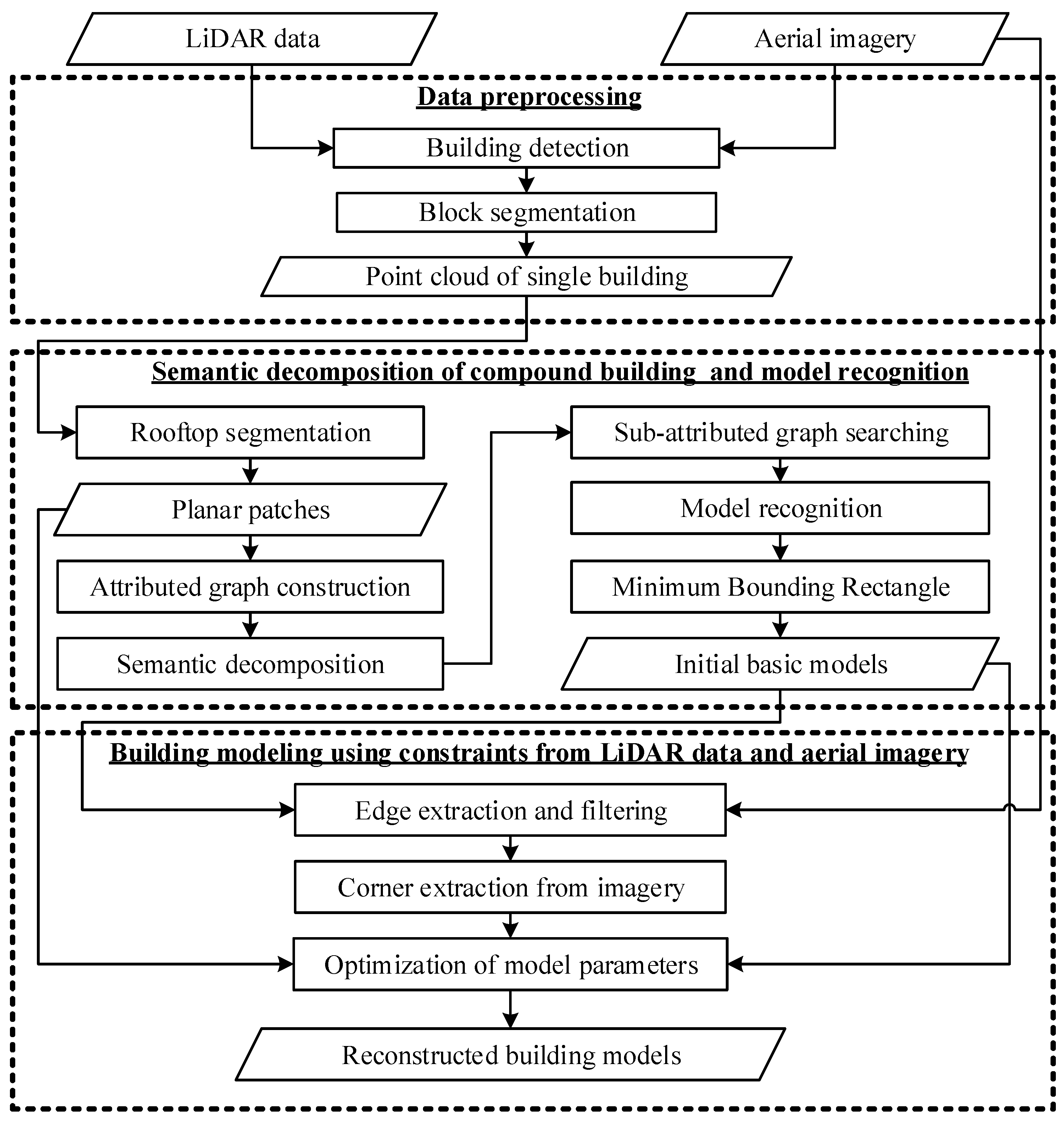
2. Methodology
2.1. Overview of the Proposed Method

2.2. Data Preprocessing
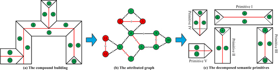
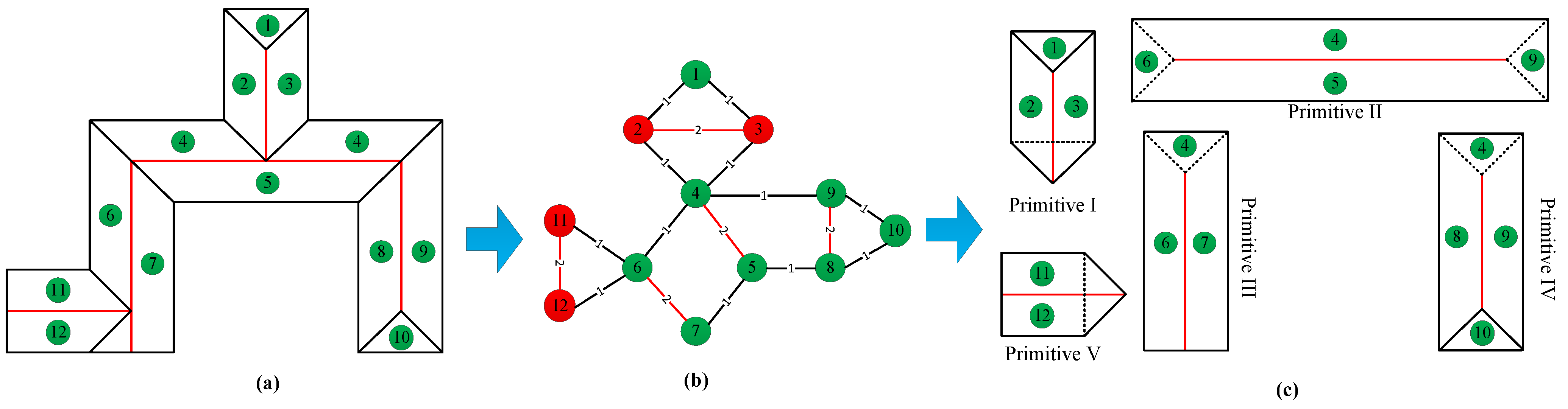
2.3. Semantic Decomposition of the Compound Building and the Primitive Recognition

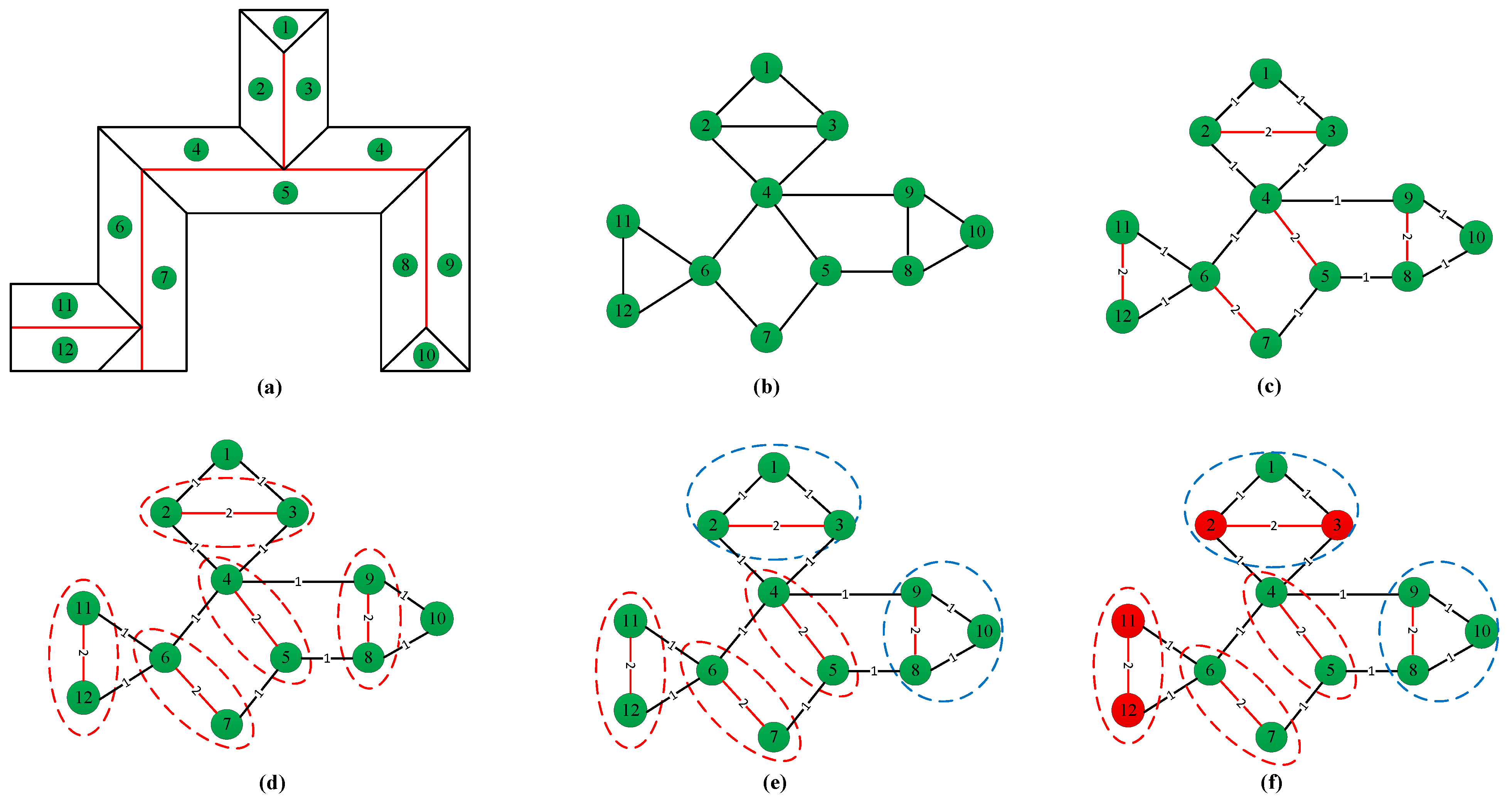
2.3.1. Construction of the Attributed Graph

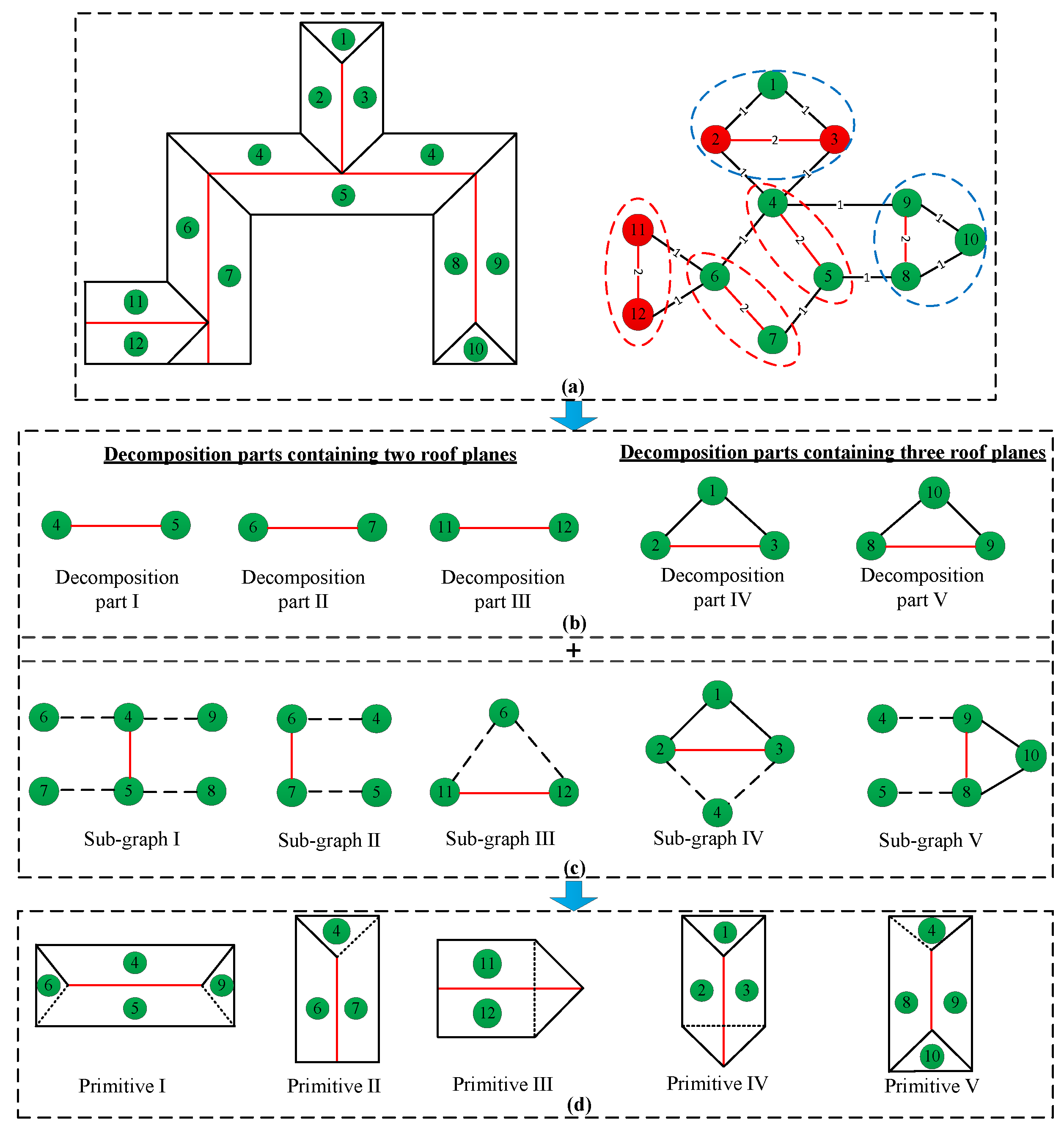
2.3.2. Sub-graph Extraction from the Attributed Graph

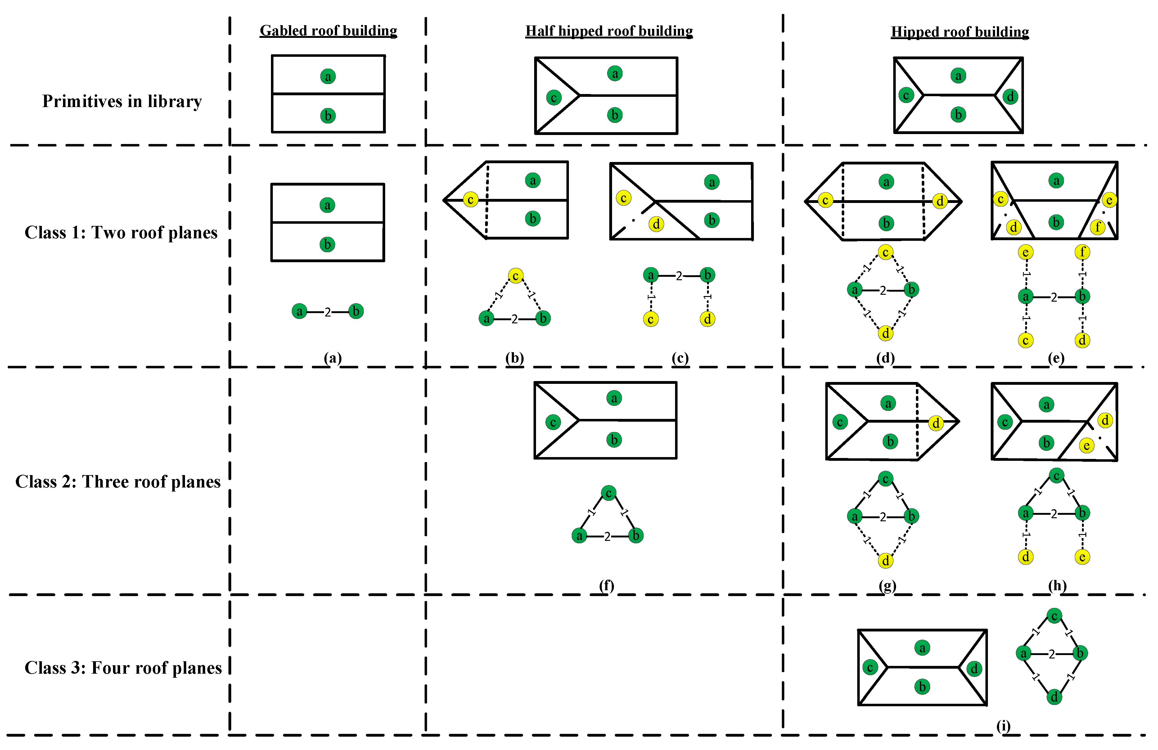
2.3.3. Primitive’s Definition and Recognition


2.3.4. Generation of Initial 3D Building Primitives

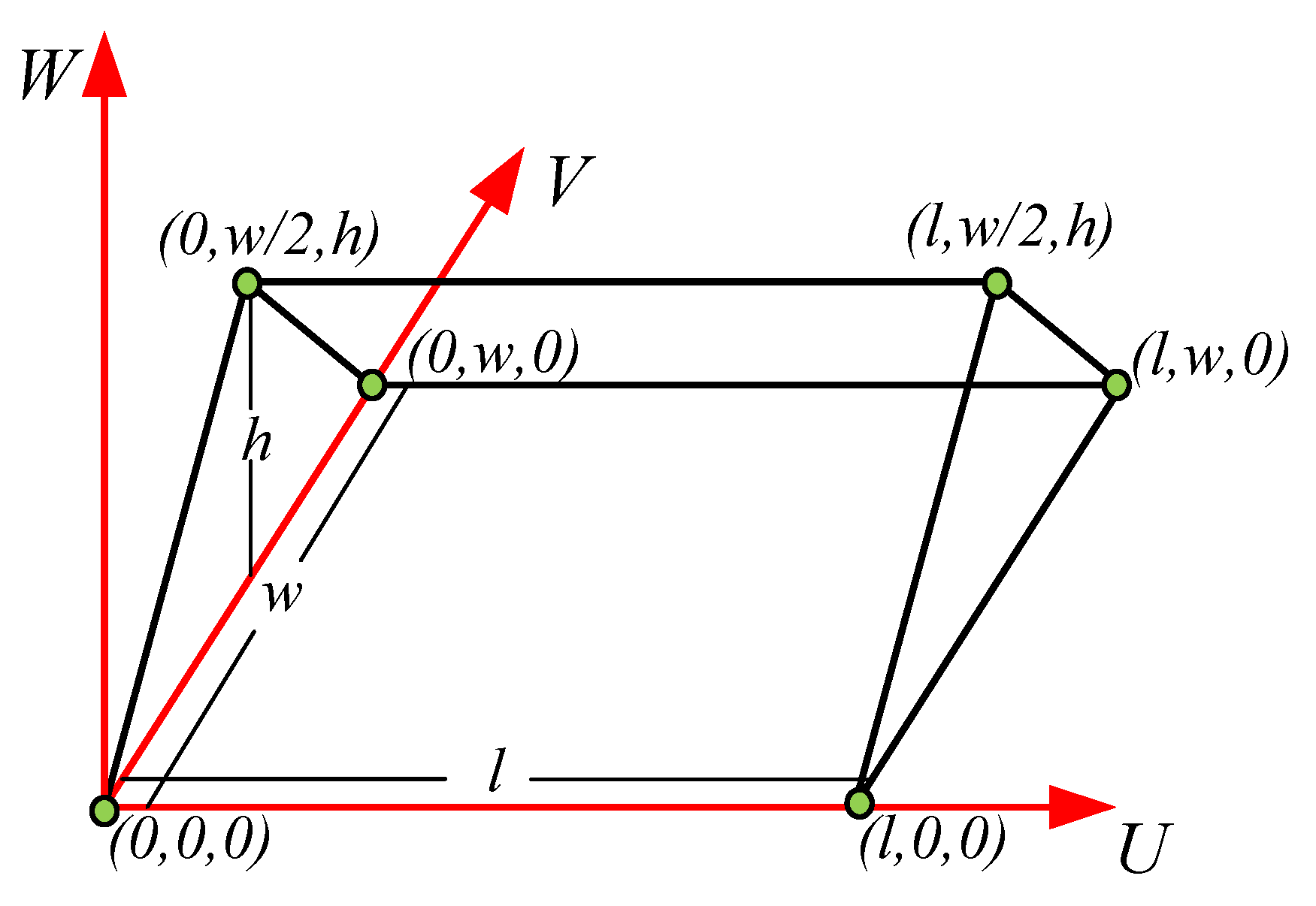
2.4. Image Feature Extraction and Building Modeling
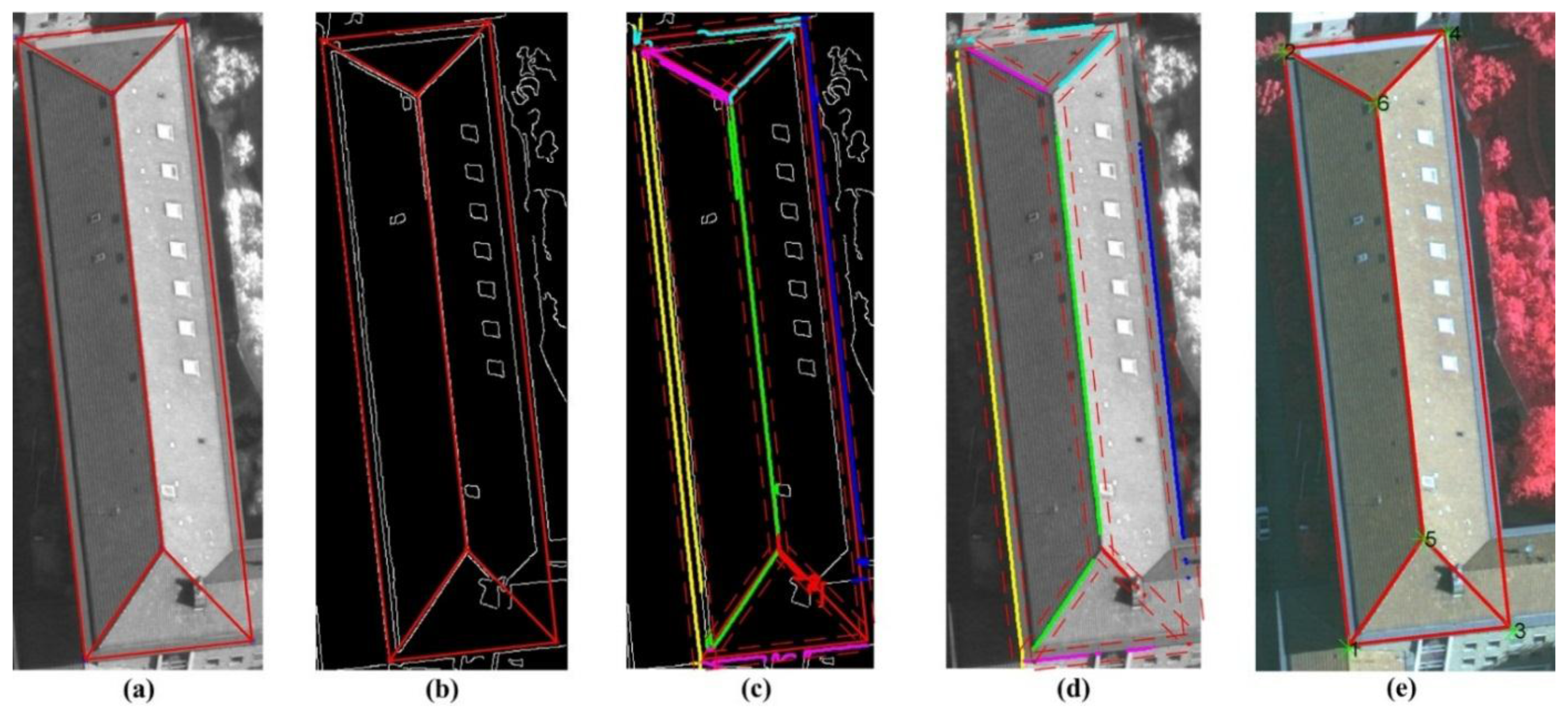
2.4.1. Feature Extraction from Perspective Aerial Imagery

2.4.2. Building Modeling Using Constraints from LiDAR Data and Perspective Aerial Imagery

3. Experimental Results
3.1. Description of the Datasets
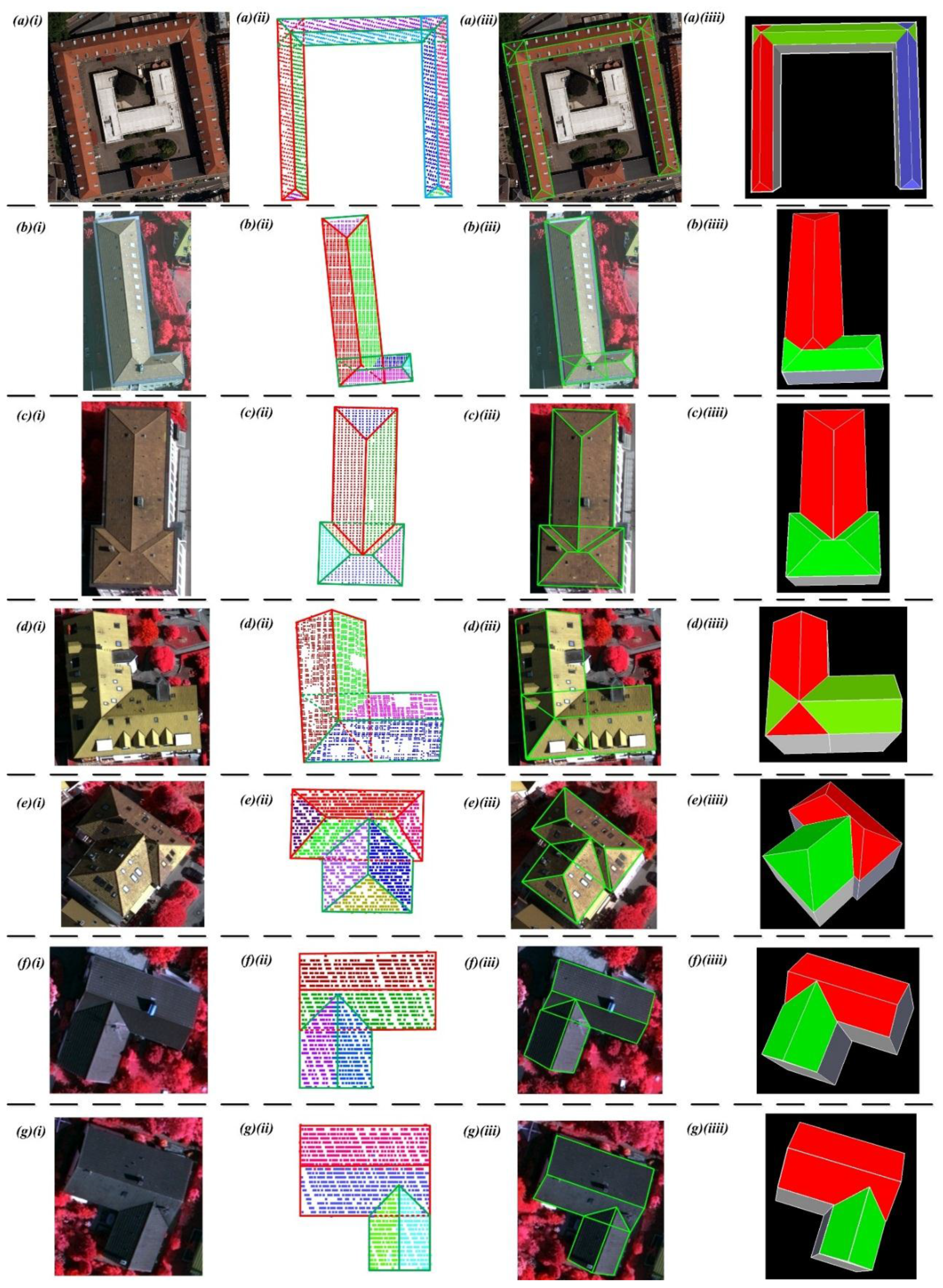
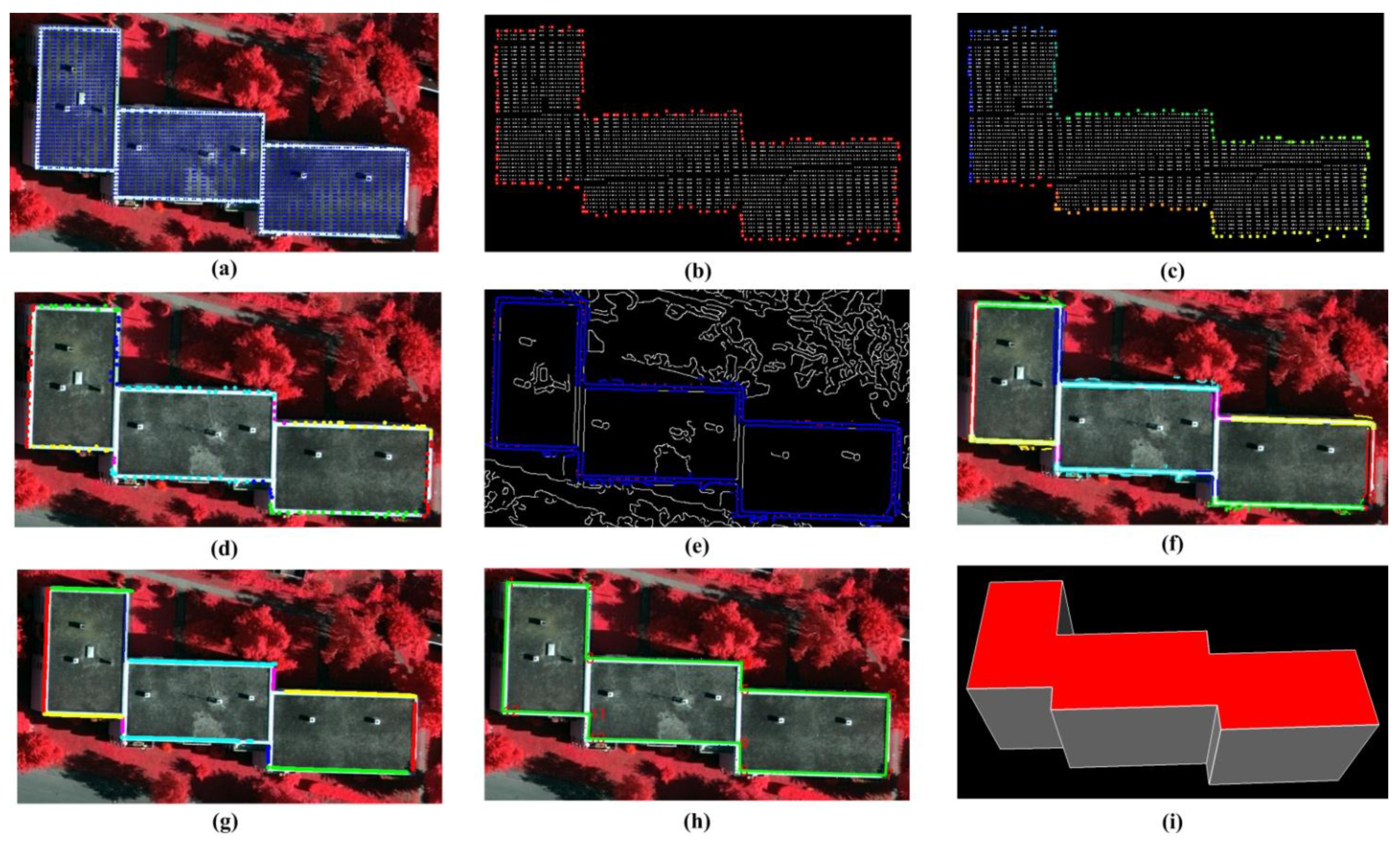
3.2. Experimental Results


4. Discussions
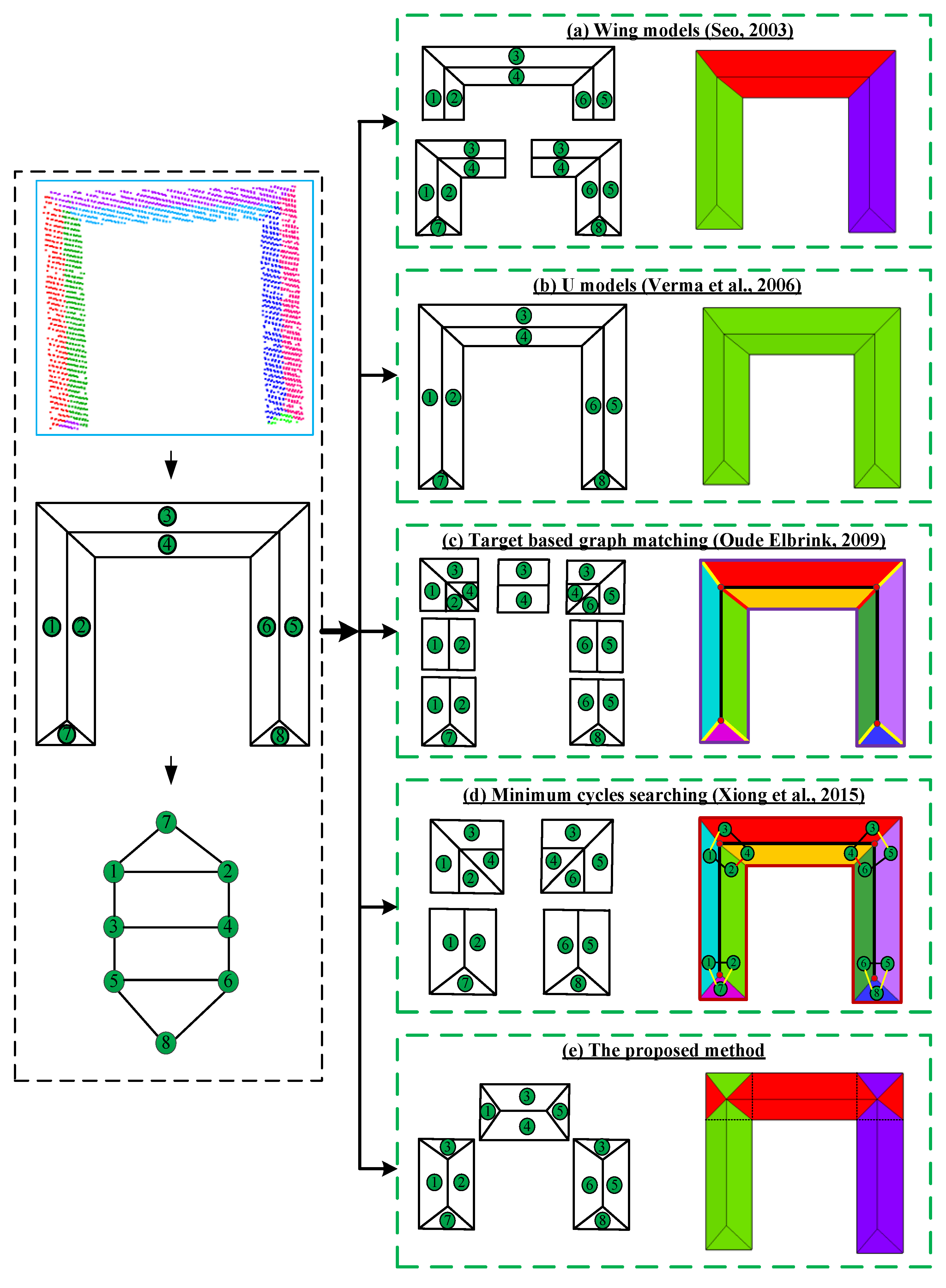
4.1. Comparison Analysis of the Proposed Semantic Decomposition Method

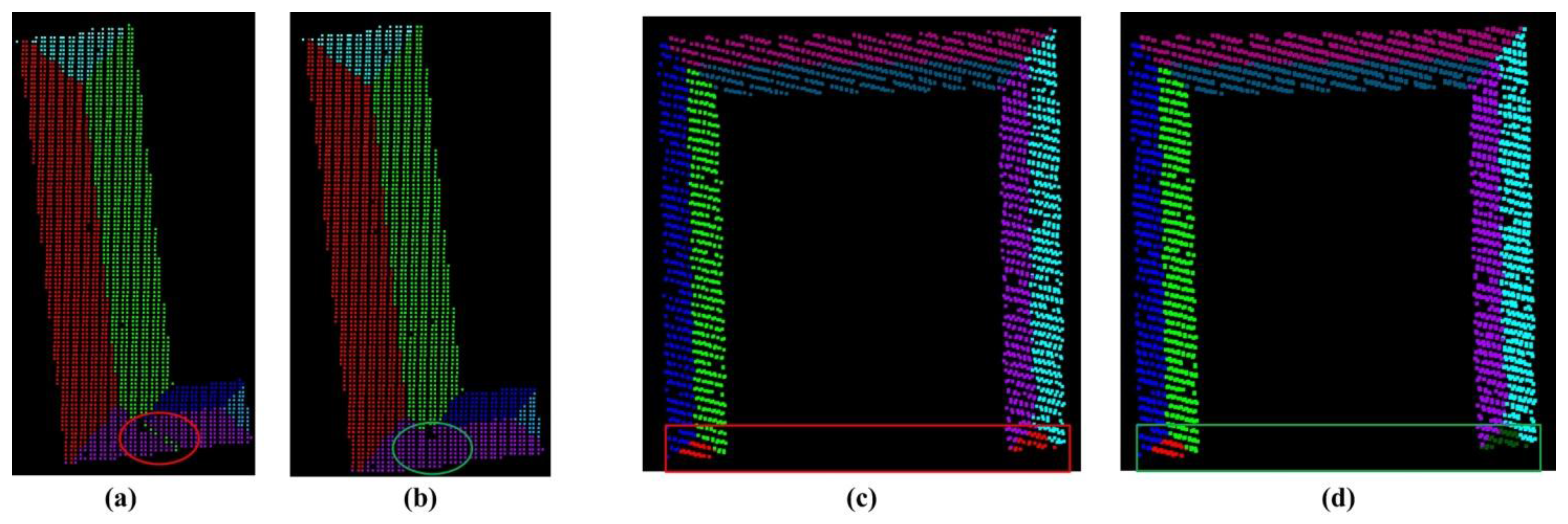
4.2. Analysis of the Sub-Graph Searching and Initial Primitive’s Generation
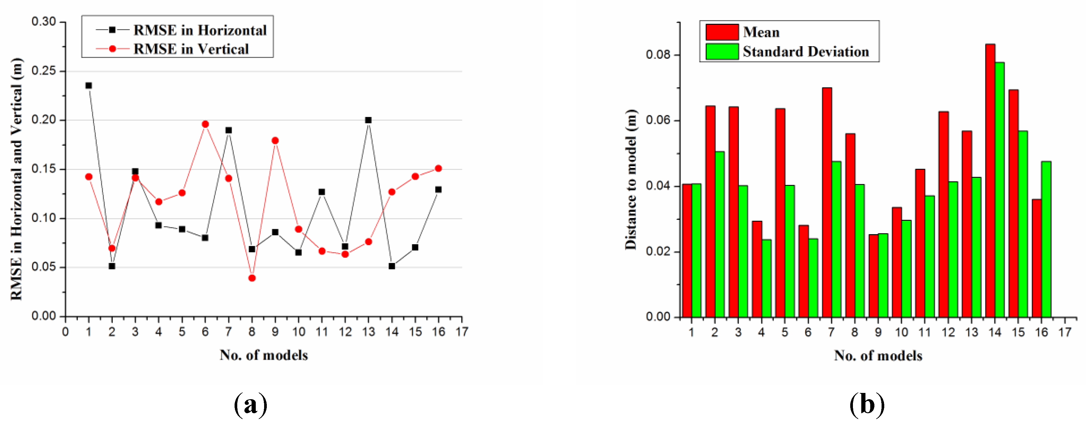
4.3. Accuracy Assessments of the Reconstructed Building Models


| Researchers and References | Area 1 | Area 2 | Area 3 | |||
|---|---|---|---|---|---|---|
| RMSD (m) | RMSZ (m) | RMSD (m) | RMSZ (m) | RMSD (m) | RMSZ (m) | |
| J.Y. Rau [55] | 0.9 | 0.6 | 0.5 | 0.7 | 0.8 | 0.6 |
| Oude Elbrink and Vosselman [37] | 0.9 | 0.2 | 1.2 | 0.1 | 0.8 | 0.1 |
| Xiong et al. [39] | 0.8 | 0.2 | 0.5 | 0.2 | 0.7 | 0.1 |
| Perera et al. [40] | 0.8 | 0.2 | 0.3 | 0.3 | 0.5 | 0.1 |
| Dorninger and Pfeifer [9] | 0.9 | 0.3 | 0.7 | 0.3 | 0.8 | 0.1 |
| Sohn et al. [56] | 0.8 | 0.3 | 0.5 | 0.3 | 0.6 | 0.2 |
| Awrangjeb et al. [19] | 0.9 | 0.2 | 0.7 | 0.3 | 0.8 | 0.1 |
| He et al. [57] | 0.7 | 0.2 | 0.6 | 0.3 | 0.7 | 0.2 |
| The proposed method | 0.8 | 0.3 | 0.5 | 0.3 | 0.6 | 0.1 |
4.4. Uncertainties and Limitations of the Proposed Method

5. Conclusions
Acknowledgments
Author Contributions
Conflicts of Interest
References
- Habib, A.F.; Zhai, R.; Kim, C. Generation of complex polyhedral building models by integrating stereo-aerial imagery and LiDAR data. Photogramm. Eng. Remote Sens. 2010, 76, 609–623. [Google Scholar] [CrossRef]
- Haala, N.; Kada, M. An update on automatic 3D building reconstruction. ISPRS J. Photogramm. Remote Sens. 2010, 65, 570–580. [Google Scholar] [CrossRef]
- Rottensteiner, F.; Briese, C. Automatic generation of building models from LiDAR data and the integration of aerial images. Int. Arch. Photogramm. Remote Sens. Spat. Inf. Sci. 2003, 34, 174–180. [Google Scholar]
- Tarsha-Kurdi, F.; Landes, T.; Grussenmeyer, P. Extended RANSAC algorithm for automatic detection of building roof planes from LiDAR data. Photogramm. J. Finl. 2008, 21, 97–109. [Google Scholar]
- Vosselman, G.; Dijkman, S. 3D building model reconstruction from point clouds and ground plans. Int. Arch. Photogramm. Remote Sens. Spat. Inf. Sci. 2001, 34, 37–44. [Google Scholar]
- Xiao, Y.; Wang, C.; Li, J.; Zhang, W.; Xi, X.; Wang, C.; Dong, P. Building segmentation and modeling from airborne LiDAR data. Int. J. Digit. Earth 2014, 5, 1–16. [Google Scholar] [CrossRef]
- Sampath, A.; Shan, J. Segmentation and reconstruction of polyhedral building roofs from aerial LiDAR point clouds. IEEE Trans. Geosci. Remote Sens. 2010, 48, 1554–1567. [Google Scholar] [CrossRef]
- Zhou, Q.Y.; Neumann, U. 2.5D building modeling by discovering global regularities. In Proceedings of the 2012 IEEE Conference on Computer Vision and Pattern Recognition(CVPR), Providence, RI, USA, 16–21 June 2012; pp. 326–333.
- Dorninger, P.; Pfeifer, N. A comprehensive automated 3D approach for building extraction, reconstruction, and regularization from airborne laser scanning point clouds. Sensors 2008, 8, 7323–7343. [Google Scholar] [CrossRef]
- You, H.J.; Zhang, S.Q. 3D building reconstruction from aerial CCD image and sparse laser sample data. Opt. Lasers Eng. 2006, 44, 555–566. [Google Scholar]
- Sohn, G.; Dowman, I. Data fusion of high-resolution satellite imagery and LiDAR data for automatic building extraction. ISPRS J. Photogramm. Remote Sens. 2007, 62, 43–63. [Google Scholar] [CrossRef]
- Seo, S. Model-Based Automatic Building Extraction from LiDAR and Aerial Imagery. Ph.D. Thesis, The Ohio State University, Columbus, OH, USA, 2003. [Google Scholar]
- Rottensteiner, F.; Trinder, J.; Clode, S.; Kubik, K. Fusing airborne laser scanner data and aerial imagery for the automatic extraction of buildings in densely built-up areas. Int. Arch. Photogramm. Remote Sens. 2004, 35, 512–517. [Google Scholar]
- Ma, R. Building Model Reconstruction from LiDAR Data and Aerial Photographs. Ph.D. Thesis, The Ohio State University, Columbus, OH, USA, 2004. [Google Scholar]
- Kim, C.J.; Habib, A. Object-based integration of photogrammetric and LiDAR data for automated generation of complex polyhedral building models. Sensors 2009, 9, 5679–5701. [Google Scholar] [CrossRef] [PubMed]
- Cheng, L.A.; Gong, J.Y.; Li, M.C.; Liu, Y.X. 3D building model reconstruction from multi-view aerial imagery and LiDAR data. Photogramm. Eng. Remote Sens. 2011, 77, 125–139. [Google Scholar] [CrossRef]
- Chen, L.C.; Teo, T.A.; Shao, Y.C.; Lai, Y.C.; Rau, J.Y. Fusion of LiDAR data and optical imagery for building modeling. Int. Arch. Photogramm. Remote Sens. 2004, 35, 732–737. [Google Scholar]
- Kwak, E. Automatic 3D Building Model Generation by Integrating LiDAR and Aerial Images Using a Hybrid Approach. Ph.D. Thesis, University of Calgary, Calgary, AB, Canada, 2013. [Google Scholar]
- Awrangjeb, M.; Zhang, C.S.; Fraser, C.S. Automatic extraction of building roofs using LiDAR data and multispectral imagery. ISPRS J. Photogramm. Remote Sens. 2013, 83, 1–18. [Google Scholar] [CrossRef]
- Brenner, C. Constraints for modelling complex objects. Int. Arch. Photogramm. Remote Sens. Spat. Inf. Sci. 2005, 36, 49–54. [Google Scholar]
- Brenner, C. Modelling 3D objects using weak CSG primitives. Int. Arch. Photogramm. Remote Sens. Spat. Inf. Sci. 2004, 35, 1085–1090. [Google Scholar]
- Verma, V.; Kumar, R.; Hsu, S. 3D building detection and modeling from aerial LiDAR data. In Proceedings of the 2006 IEEE Conference on Computer Vision and Pattern Recognition(CVPR), New York, NY, USA, 17–22 June 2006; pp. 2213–2220.
- Maas, H.G.; Vosselman, G. Two algorithms for extracting building models from raw laser altimetry data. ISPRS J. Photogramm. Remote Sens. 1999, 54, 153–163. [Google Scholar] [CrossRef]
- Kada, M.; McKinley, L. 3D building reconstruction from lidar based on a cell decomposition approach. Int. Arch. Photogramm. Remote Sens. Spat. Inf. Sci. 2009, 38, 47–52. [Google Scholar]
- Henn, A.; Groger, G.; Stroh, V.; Plumer, L. Model driven reconstruction of roofs from sparse LiDAR point clouds. ISPRS J. Photogramm. Remote Sens. 2013, 76, 17–29. [Google Scholar] [CrossRef]
- Haala, N.; Brenner, C. Extraction of buildings and trees in urban environments. ISPRS J. Photogramm. Remote Sens. 1999, 54, 130–137. [Google Scholar] [CrossRef]
- Tseng, Y.H.; Wang, S.D. Semi-automated building extraction based on CSG model-image fitting. Photogramm. Eng. Remote Sens. 2003, 69, 171–180. [Google Scholar] [CrossRef]
- Suveg, D.; Vosselman, G. Reconstruction of 3D building models from aerial images and maps. ISPRS J. Photogramm. Remote Sens. 2004, 58, 202–224. [Google Scholar] [CrossRef]
- Lafarge, F.; Descombes, X.; Zerubia, J.; Pierrot-Deseilligny, M. Structural approach for building reconstruction from a single DSM. IEEE Trans. Pattern Anal. Mach. Intell. 2008, 32, 135–147. [Google Scholar] [CrossRef] [PubMed] [Green Version]
- Huang, H.; Brenner, C.; Sester, M. A generative statistical approach to automatic 3D building roof reconstruction from laser scanning data. ISPRS J. Photogramm. Remote Sens. 2013, 79, 29–43. [Google Scholar] [CrossRef]
- Vosselman, G.; Veldhuis, H. Mapping by dragging and fitting of wire-frame models. Photogramm. Eng. Remote Sens. 1999, 65, 769–776. [Google Scholar]
- Durupt, M.; Taillandier, F. Automatic building reconstruction from a digital elevation model and cadastral data: An operational approach. Int. Arch. Photogramm. Remote Sens. Spat. Inf. Sci. 2006, 36, 142–147. [Google Scholar]
- Wang, S.; Tseng, Y.H. Least squares model image fitting of floating models for building extraction from images. J. Chin. Inst. Eng. 2009, 32, 667–677. [Google Scholar] [CrossRef]
- Gruen, A.; Wang, X. Cc-modeler: A topology generator for 3D city models. ISPRS J. Photogramm. Remote Sens. 1998, 53, 286–295. [Google Scholar] [CrossRef]
- Wang, S.; Tseng, Y.H.; Chen, L.C. Semi-automated model-based building reconstruction by fitting models to versatile data. In Proceedings of the 29th Asian Conference on Remote Sensing, Colombo, Sri Lanka, 10–14 November 2008.
- Haala, N.; Becker, S.; Kada, M. Cell decomposition for the generation of building models at multiple scales. Int. Arch. Photogramm. Remote Sens. Spat. Inf. Sci. 2006, 36, 19–24. [Google Scholar]
- Oude Elberink, S.; Vosselman, G. Building reconstruction by target based graph matching on incomplete laser data: Analysis and limitations. Sensors 2009, 9, 6101–6118. [Google Scholar] [CrossRef] [PubMed]
- Lin, H.; Gao, J.Z.; Zhou, Y.; Lu, G.L.; Ye, M.; Zhang, C.X.; Liu, L.G.; Yang, R.G. Semantic decomposition and reconstruction of residential scenes from LiDAR data. ACM Trans. Graph. 2013, 32, 6601–6610. [Google Scholar] [CrossRef]
- Xiong, B.; Oude Elberink, S.; Vosselman, G. A graph edit dictionary for correcting errors in roof topology graphs reconstructed from point clouds. ISPRS J. Photogramm. Remote Sens. 2014, 93, 227–242. [Google Scholar] [CrossRef]
- Perera, G.S.N.; Maas, H.G. Cycle graph analysis for 3D roof structure modelling: Concepts and performance. ISPRS J. Photogramm. Remote Sens. 2014, 93, 213–226. [Google Scholar] [CrossRef]
- Zhang, W.; Wang, H.; Chen, Y.; Yan, K.; Chen, M. 3D building roof modeling by optimizing primitive’s parameters using constraints from lidar data and aerial imagery. Remote Sens. 2014, 6, 8107–8133. [Google Scholar] [CrossRef]
- Axelsson, P. DEM generation from laser scanner data using adaptive TIN models. Int. Arch. Photogramm. Remote Sens. 2000, 33, 111–118. [Google Scholar]
- Rusu, R.B. Semantic 3D object maps for everyday manipulation in human living environments. Künstl. Intell. 2010, 24, 345–348. [Google Scholar] [CrossRef]
- Chen, D.; Zhang, L.; Li, J.; Liu, R. Urban building roof segmentation from airborne LiDAR point clouds. Int. J. Remote Sens. 2012, 33, 6497–6515. [Google Scholar] [CrossRef]
- Edelsbrunner, H.; Kirkpatrick, D.; Seidel, R. On the shape of a set of points in the plane. IEEE Trans. Inf. Theory 1983, 29, 551–559. [Google Scholar] [CrossRef]
- Chaudhuri, D.; Samal, A. A simple method for fitting of bounding rectangle to closed regions. Pattern Recognit. 2007, 40, 1981–1989. [Google Scholar] [CrossRef]
- Canny, J. A computational approach to edge detection. IEEE Trans. Pattern Anal. Mach. Intell. 1986, 8, 679–698. [Google Scholar] [CrossRef] [PubMed]
- Fischler, M.A.; Bolles, R.C. Random sample consensus: A paradigm for model fitting with applications to image analysis and automated cartography. Commun. ACM 1981, 24, 381–395. [Google Scholar] [CrossRef]
- Marquardt, D.W. An algorithm for least-squares estimation of nonlinear parameters. J. Soc. Ind. Appl. Math. 1963, 11, 431–441. [Google Scholar] [CrossRef]
- ISPRS Test Project on Urban Classification and 3D Building Reconstruction. Available online: http://www.itc.nl/isprs_wgiii4/docs/complexscenes.pdf (accessed on 7 August 2015).
- Sampath, A.; Shan, J. Building boundary tracing and regularization from airborne LiDAR point clouds. Photogramm. Eng. Remote Sens. 2007, 73, 805–812. [Google Scholar] [CrossRef]
- Xiong, B.; Jancosek, M.; Oude Elberink, S.; Vosselman, G. Flexible building primitives for 3D building modeling. ISPRS J. Photogramm. Remote Sens. 2015, 101, 275–290. [Google Scholar] [CrossRef]
- Rottensteiner, F.; Sohn, G.; Gerke, M.; Wegner, J.D.; Breitkopf, U.; Jung, J. Results of the ISPRS benchmark on urban object detection and 3D building reconstruction. ISPRS J. Photogramm. Remote Sens. 2013, 93, 256–271. [Google Scholar] [CrossRef]
- ISPRS Test Project on Urban Classification and 3D Building Reconstruction: Results. Available online: http://brian94.de/ISPRSIII_4_Test_results/tests_datasets_results_main.html (accseesed on 30 July 2015).
- Rau, J.Y. A line-based 3D roof modell reconstruction algorithm: TIN-merging and reshaping (TMR). In Proceedings of the ISPRS Annals of the Photogrammetry, Remote Sensing and Spatial Information Sciences, Melbourne, Australia, 25 August–1 September 2012; pp. 287–292.
- Sohn, G.; Huang, X.F.; Tao, V. Using a binary space partitioning tree for reconstructing polyhedral building models from airborne LiDAR data. Photogramm. Eng. Remote Sens. 2008, 74, 1425–1438. [Google Scholar] [CrossRef]
- He, Y.; Zhang, C.; Fraser, C. A line-based spectral clustering method for efficient planar structure extraction from lidar data. In Proceedings of ISPRS Annals of the Photogrammetry, Remote Sensing and Spatial Information Sciences, Antalya, Turkey, 11–13 November 2013; pp. 103–108.
© 2015 by the authors; licensee MDPI, Basel, Switzerland. This article is an open access article distributed under the terms and conditions of the Creative Commons Attribution license (http://creativecommons.org/licenses/by/4.0/).
Share and Cite
Wang, H.; Zhang, W.; Chen, Y.; Chen, M.; Yan, K. Semantic Decomposition and Reconstruction of Compound Buildings with Symmetric Roofs from LiDAR Data and Aerial Imagery. Remote Sens. 2015, 7, 13945-13974. https://0-doi-org.brum.beds.ac.uk/10.3390/rs71013945
Wang H, Zhang W, Chen Y, Chen M, Yan K. Semantic Decomposition and Reconstruction of Compound Buildings with Symmetric Roofs from LiDAR Data and Aerial Imagery. Remote Sensing. 2015; 7(10):13945-13974. https://0-doi-org.brum.beds.ac.uk/10.3390/rs71013945
Chicago/Turabian StyleWang, Hongtao, Wuming Zhang, Yiming Chen, Mei Chen, and Kai Yan. 2015. "Semantic Decomposition and Reconstruction of Compound Buildings with Symmetric Roofs from LiDAR Data and Aerial Imagery" Remote Sensing 7, no. 10: 13945-13974. https://0-doi-org.brum.beds.ac.uk/10.3390/rs71013945