
A Spectral Unmixing Model for the Integration of Multi-Sensor Imagery: A Tool to Generate Consistent Time Series Data


Abstract
:
1. Introduction
2. Methodology

2.1. Unsupervised Fuzzy Classification
2.2. Spectral Unmixing Concept
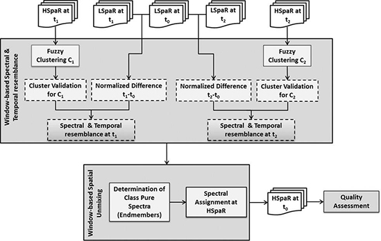
- The class contribution to the LSpaR image pixel, , which is the proportion of each class in the LSpaR image pixel and is estimated using membership values to the corresponding class k. Explicitly, is the average of all the class contributions to LSpaR pixel footprint N, according to Equation (3). The critical issue in this case pertains to ensuring accurate co-registration between the images. In this study, the LSpaR image pixel footprint is resampled on HSpaR image pixel size, considering that the point spread function (PSF) is rectangular. Therefore, N is the total number of HSpaR image pixels i within the LSpaR image pixel footprint.
- The spectral difference between the LSpaR image of the predicted date t0 and that of each of the base dates t1 and t2, in order to handle changes between multitemporal observations efficiently. Based on these differences, the normalized temporal weights and are calculated for every pixel in the window (Equation (4)) and being later involved in the unmixing process.The temporal weights and are estimated per window, the weights being assigned to the central pixel of the sliding window with size w. The least changes occurred between the two dates, the greater the similarity between the corresponding image pixels and thus the higher the value of the temporal weight T for the selected pixel.
3. Experimental Results and Evaluation
3.1. Dataset and Study Area


| MODIS Bands MOD09GA L2G | MODIS Bandwidth (nm) | SPOT4 Bands Level 2A | SPOT Bandwidth (nm) |
|---|---|---|---|
| Band 3/Blue | 459–479 | ||
| Band 4/Green | 545–565 | XS1/Green | 500–590 |
| Band 1/Red | 620–670 | XS2/Red | 610–680 |
| Band 2/NIR | 841–876 | XS3/NIR | 790–890 |
| Band 6/SWIR1 | 1628–1652 | SWIR | 1530–1750 |
| Band 7/SWIR2 | 2105–2155 | ||

| Imagery | Acquisition Dates | Usage | Spatial Resolution Radiometric Values | Geometric Reference | |
|---|---|---|---|---|---|
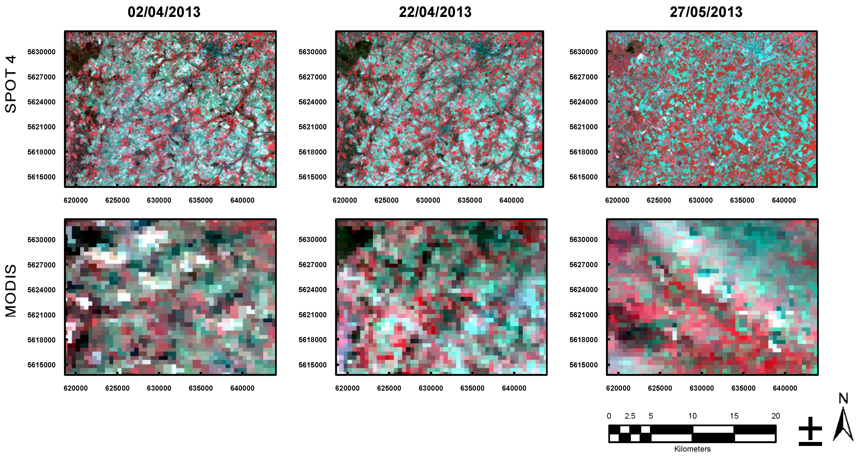
| MODIS MOD09GA L2G | 2 April 2013 | Unmixing | 500 m | Surface Reflectance | Map Projection: UTM Ellipsoid Type: WGS84 |
| 22 April 2013 | Unmixing | ||||
| 27 May 2013 | Unmixing | ||||
| SPOT4 (Take 5) Level 2A | 2 April 2013 | Classification | 20 m | ||
| 22 April 2013 | Validation | ||||
| 27 May 2013 | Classification | ||||
3.2. Clustering Results and Optimal Cluster Number
| Optimal Value | 15 | 16 | 17 | 18 | 19 | 20 | 21 | 22 | 23 | 24 | 25 | 26 | 27 | ||
| Criteria | |||||||||||||||
| FHV e-06 | min | 3.34 | 3.10 | 3.90 | 3.93 | 3.88 | 4.81 | 4.82 | 4.73 | 4.80 | 4.85 | 5.14 | 5.19 | 5.20 | |
| PD e+05 | max | 14.77 | 15.21 | 15.92 | 16.44 | 16.87 | 17.34 | 18.80 | 19.28 | 20.75 | 21.18 | 22.54 | 23.96 | 24.80 | |
| SC | max | 0.82 | 0.87 | 0.82 | 0.89 | 0.92 | 0.92 | 0.94 | 0.93 | 0.95 | 0.94 | 0.93 | 0.90 | 0.92 | |
| S e-07 | min | 9.49 | 10.96 | 10.59 | 11.86 | 11.91 | 12.30 | 12.22 | 12.31 | 12.41 | 13.07 | 13.85 | 13.35 | 13.73 | |
| XB | min | 8.24 | 7.59 | 6.49 | 6.51 | 5.54 | 5.14 | 5.43 | 4.15 | 4.24 | 4.24 | 4.00 | 3.61 | 3.36 | |
| Optimal Value | 28 | 29 | 30 | 31 | 32 | 33 | 34 | 35 | 36 | 37 | 38 | 39 | 40 | ||
| Criteria | |||||||||||||||
| Fhv e-06 | min | 5.25 | 5.00 | 4.74 | 4.54 | 4.37 | 3.91 | 4.03 | 4.21 | 4.39 | 4.32 | 4.17 | 4.15 | 4.16 | |
| PD e+05 | max | 25.18 | 26.86 | 28.51 | 29.66 | 31.17 | 33.72 | 30.81 | 30.91 | 30.94 | 30.98 | 30.06 | 30.13 | 39.21 | |
| SC | max | 0.94 | 0.95 | 0.93 | 0.95 | 0.94 | 0.98 | 0.95 | 0.96 | 0.98 | 1.00 | 0.98 | 0.99 | 0.99 | |
| S e-07 | min | 13.59 | 13.75 | 13.13 | 13.67 | 13.33 | 12.92 | 13.48 | 13.87 | 14.01 | 14.15 | 13.75 | 13.99 | 14.00 | |
| XB | min | 3.97 | 3.60 | 3.41 | 3.10 | 3.04 | 2.57 | 2.89 | 3.01 | 2.99 | 3.07 | 2.39 | 2.39 | 2.52 | |
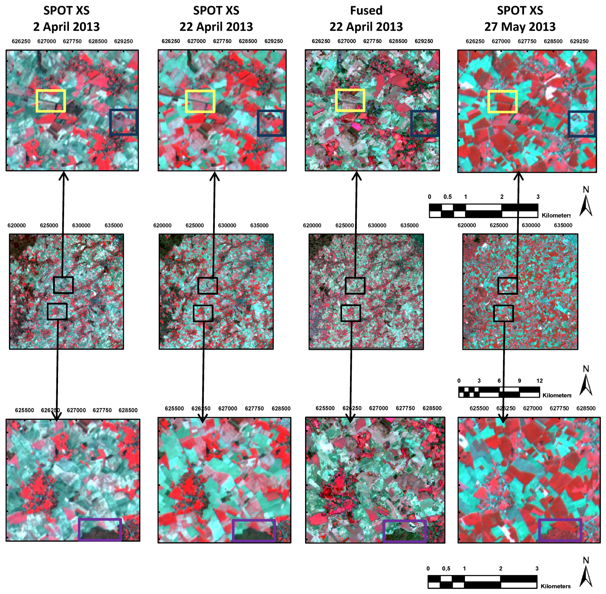
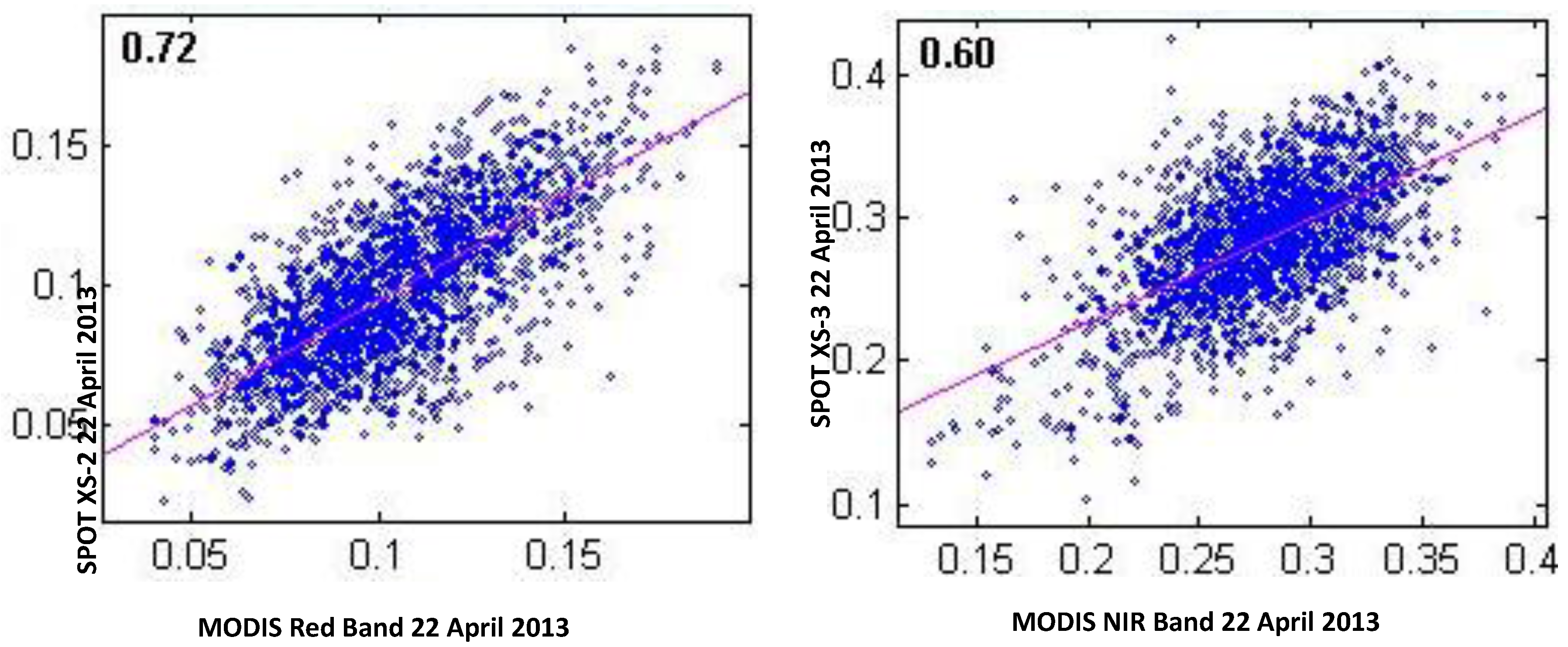
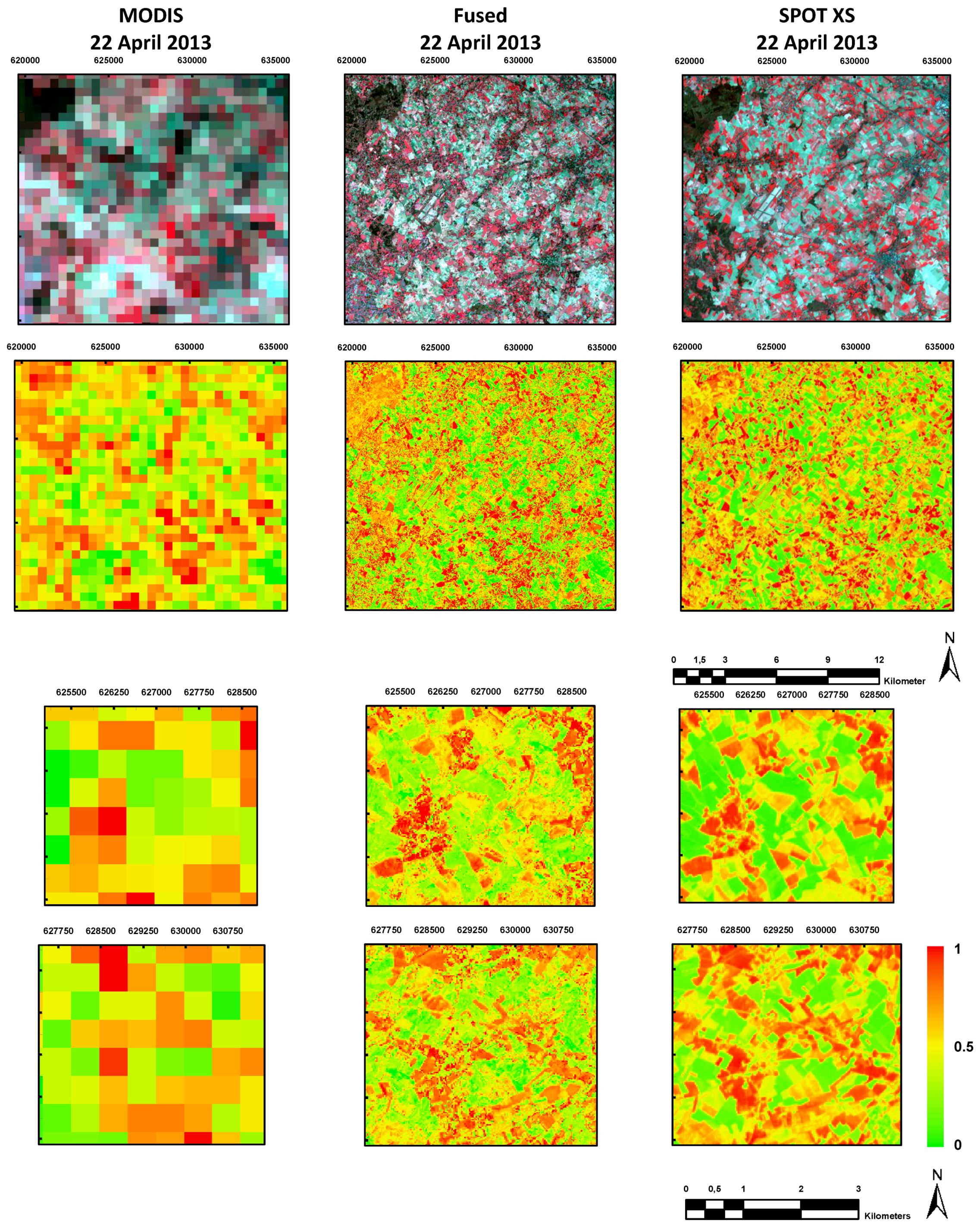
3.3. Spectral-Unmixing Fusion

| Bands | RMSE | ERGAS_S | CORR | Q4 | AvAbsDiff | AvDiff |
|---|---|---|---|---|---|---|
| Green | 0.0281 | 0.612 | 0.7808 | 0.686 | 0.0229 | −0.0131 |
| Red | 0.0296 | 0.7961 | 0.0241 | −0.0009 | ||
| NIR | 0.0458 | 0.7443 | 0.0413 | 0.0201 | ||
| SWIR | 0.0496 | 0.7477 | 0.0409 | −0.0142 |


3.4. Implementation on the Upcoming Data of Sentinel-2 MSI and Sentinel-3 OLCI
4. Conclusions
- The automatic definition of the optimal cluster number with the help of various evaluation criteria, establishing a faster and more robust methodology. The previous approaches required a trial-and-error process in this methodology step, meaning that the unmixing algorithm had to be tested in a range of cluster numbers. By evaluating the unmixing result for each of the different clustering output in those cases, the corresponding cluster number was defined. Estimating the optimal cluster number, without the need to implement the unmixing algorithm in this study, reduces the execution time of the entire process.
- The temporal weights embedded in the algorithm, enabling the efficient handling of the changes occurred between the study dates. The available HSpaR images are classified separately and the temporal weights define the contribution of every land cover type to the pixel of the LSpaR image to be unmixed. The advantage in this case is twofold; firstly the unmixing algorithm is able to determine the state of the land cover type on the prediction date and secondly this is feasible with only one implementation. In previous approaches, the temporal weights are implemented in the unmixing outputs of the two base dates and subsequent estimations of reflectances are required on the prediction date [14].
Acknowledgments
Author Contributions
Conflicts of Interest
References
- Drusch, M.; Del Bello, U.; Carlier, S.; Colin, O.; Fernandez, V.; Gascon, F.; Hoersch, B.; Isola, C.; Laberinti, P.; Martimort, P.; et al. Sentinel-2: ESA’s optical high-resolution mission for GMES operational services. Remote Sens. Environ. 2012, 120, 25–36. [Google Scholar] [CrossRef]
- Zhukov, B.; Oertel, D.; Lanzl, F.; Reinhäckel, G. Unmixing-based multi sensor multi-resolution image fusion. IEEE Trans. Geosci. Remote Sens. 1999, 37, 1212–1226. [Google Scholar] [CrossRef]
- Minghelli-Roman, A.; Polidori, L.; Mathieu-Blanc, S.; Loubersac, L.; Cauneau, F. Spatial resolution improvement by merging MERIS-ETM images for coastal water monitoring. IEEE Geosci. Remote Sens. Lett. 2006, 3, 227–231. [Google Scholar] [CrossRef]
- Zurita-Milla, R.; Kaiser, G.; Clevers, J.G.P.W.; Schneider, W.; Schaepman, M.E. Downscaling time series of MERIS full resolution data to monitor vegetation seasonal dynamics. Remote Sens. Environ. 2009, 9, 1874–1885. [Google Scholar] [CrossRef]
- Zurita-Milla, R.; Gómez-Chova, L.; Guanter, L.; Clevers, J.G.P.W.; Camps-Valls, G. Multitemporal unmixing of medium-spatial-resolution satellite images: A case study using MERIS images for land-cover mapping. IEEE Trans. Geosci. Remote Sens. 2011, 11, 4308–4317. [Google Scholar] [CrossRef]
- Amorós-López, J.; Gómez-Chova, L.; Guanter, L.; Alonso, L.; Moreno, J.; Camps-Valls, G. Regularized multiresolution spatial unmixing for ENVISAT/MERIS and Landsat/TM image Fusion. IEEE Geosci. Remote Sens. Lett. 2011, 5, 844–848. [Google Scholar] [CrossRef]
- Amorós-López, J.; Gómez-Chova, L.; Alonso, L.; Guanter, L.; Zurita-Milla, R.; Moreno, J.; Camps-Valls, G. Multitemporal fusion of Landsat/TM and ENVISAT/MERIS for crop monitoring. Int. J. Appl. Earth Observ. Geoinf. 2013, 23, 132–141. [Google Scholar] [CrossRef]
- Gao, F.; Masek, J.; Schwaller, M.; Hall, F. On the blending of the Landsat and MODIS surface reflectance: Predicting daily Landsat surface reflectance. IEEE Trans. Geosci. Remote Sens. 2006, 44, 2207–2218. [Google Scholar]
- Hilker, T.; Wulder, M.A.; Coops, N.C.; Linke, J.; McDermid, G.; Masek, J.; Gao, F.; White, J.C. A new data fusion model for high spatial- and temporal-resolution mapping of forest based on Landsat and MODIS. Remote Sens. Environ. 2009, 113, 1613–1627. [Google Scholar] [CrossRef]
- Walker, J.J.; de Beurs, K.M.; Wynne, R.H.; Gao, F. Evaluation of Landsat and MODIS data fusion products for analysis of dryland forest phenology. Remote Sens. Environ. 2012, 117, 381–393. [Google Scholar] [CrossRef]
- Jarihani, A.A.; McVicar, T.R.; Van Niel, T.G.; Emelyanova, I.V.; Callow, J.N.; Johansen, K. Blending Landsat and MODIS data to generate multispectral indices: A comparison of “Index-then-Blend” and “Blend-then-Index” approaches. Remote Sens. 2014, 6, 9213–9238. [Google Scholar] [CrossRef] [Green Version]
- Zhu, X.; Chen, J.; Gao, F.; Chen, X.; Masek, J.G. An enhanced spatial and temporal adaptive reflectance fusion model for complex heterogeneous regions. Remote Sens. Environ. 2010, 114, 2610–2623. [Google Scholar] [CrossRef]
- Hilker, T.; Wulder, M.A.; Coops, N.C.; Sritz, N.; White, J.C.; Gao, F.; Masek, J.G.; Stenhouse, G. Generation of dense time series synthetic Landsat data through data blending with MODIS using a spatial and temporal adaptive reflectance fusion model. Remote Sens. Environ. 2009, 113, 1988–1999. [Google Scholar] [CrossRef]
- Zhang, W.; Li, A.; Jin, H.; Bian, J.; Zhang, Z.; Lei, G.; Huang, C. An enhanced spatial and temporal data fusion model for fusing Landsat and MODIS surface reflectance to generate high temporal Landsat-like data. Remote Sens. 2013, 5, 5346–5368. [Google Scholar] [CrossRef]
- Gath, I.; Geva, A.B. Unsupervised optimal fuzzy clustering. IEEE Trans. Pattern Anal. Machine Intell. 1989, 7, 773–781. [Google Scholar] [CrossRef]
- Tso, B.; Mather, P.M. Classification Methods for Remotely Sensed Data, 2nd ed.; Taylor and Francis: New York, NY, USA, 2009. [Google Scholar]
- Bensaid, A.M.; Hall, L.O.; Bezdek, J.C.; Clarke, L.P.; Silbiger, M.L.; Arrington, J.A.; Murtagh, R.F. Validity-guided (Re)clustering with applications to image segmentation. IEEE Trans. Fuzzy Syst. 1996, 4, 112–123. [Google Scholar] [CrossRef]
- Kim, D.W.; Lee, K.H.; Lee, D. On cluster validity index for estimation of the optimal number of fuzzy clusters. Pattern Recognit. 2004, 37, 2009–2025. [Google Scholar] [CrossRef]
- Balasko, B.; Abonyi, J.; Feil, B. Fuzzy Clustering and Data Analysis Toolbox (for Use with Matlab). Available Online: http://www.abonyilab.com/software-and-data/fclusttoolbox/ (accessed on 23 July 2013).
- Wang, W.; Zhang, Y. On fuzzy cluster validity indices. Fuzzy Sets Syst. 2007, 19, 2095–2117. [Google Scholar] [CrossRef]
- Hagolle, O.; Huc, M.; Kadiri, M.; Inglada, J.; Marais-Sicre, C.; Dedieu, G.; Sylvander, S.; Leroy, M.; Meygret, A.; Lonjou, V.; et al. SPOT4 (Take 5) time series over 45 sites to get ready for Sentinel-2. In Presentation of lessons learned from SPOT4 -Take5 at S2 Symposium, Rome, Italy, 20–22 May 2014.
- Wald, L. Data Fusion, Definition and Architectures: Fusion of Image of Different Spatial Resolutions; Presses des MINES: Paris, France, 2002. [Google Scholar]
- Alparone, L.; Baronti, S.; Garzelli, A.; Nencini, F. A global quality measurement of Pan-sharpened multispectral imagery. IEEE Geosci. Remote Sens. Lett. 2004, 4, 313–317. [Google Scholar] [CrossRef]
- Inglada, J. Automatic land-cover map production of agricultural areas using supervised classification of SPOT4 (Take5) and Landsat-8 image time series. In Presentation from SPOT4 -Take5 users day, CNES Toulouse, France, 18–19 November 2014.
- Khavarian, H; Atkinson, P.M.; Milton, E.J.; Stewart, J.B. Validation of the MODIS reflectance product under UK products. Int. J. Remote Sens. 2013, 34, 7376–7399. [Google Scholar]
- Gevaert, C.M.; García-Haro, F.J. A comparison of STARFM and an unmixing-based algorithm for Landsat and MODIS data fusion. Remote Sens. Environ. 2015, 156, 34–44. [Google Scholar] [CrossRef]
© 2015 by the authors; licensee MDPI, Basel, Switzerland. This article is an open access article distributed under the terms and conditions of the Creative Commons Attribution license (http://creativecommons.org/licenses/by/4.0/).
Share and Cite
Doxani, G.; Mitraka, Z.; Gascon, F.; Goryl, P.; Bojkov, B.R. A Spectral Unmixing Model for the Integration of Multi-Sensor Imagery: A Tool to Generate Consistent Time Series Data. Remote Sens. 2015, 7, 14000-14018. https://0-doi-org.brum.beds.ac.uk/10.3390/rs71014000
Doxani G, Mitraka Z, Gascon F, Goryl P, Bojkov BR. A Spectral Unmixing Model for the Integration of Multi-Sensor Imagery: A Tool to Generate Consistent Time Series Data. Remote Sensing. 2015; 7(10):14000-14018. https://0-doi-org.brum.beds.ac.uk/10.3390/rs71014000
Chicago/Turabian StyleDoxani, Georgia, Zina Mitraka, Ferran Gascon, Philippe Goryl, and Bojan R. Bojkov. 2015. "A Spectral Unmixing Model for the Integration of Multi-Sensor Imagery: A Tool to Generate Consistent Time Series Data" Remote Sensing 7, no. 10: 14000-14018. https://0-doi-org.brum.beds.ac.uk/10.3390/rs71014000