Multi-Image and Multi-Sensor Change Detection for Long-Term Monitoring of Arid Environments With Landsat Series

Abstract

An automated procedure has been proposed to monitor by multispectral satellite imagery the cultivation expansion between 1987 and 2013 in the arid environment of the Fayyum Oasis (Egypt), which is subject to land reclamation. A change detection procedure was applied to the four years investigated (1987, 1998, 2003 and 2013). This long-term analysis is based on images from the Landsat series, adopting a classification strategy relying on vegetation index computations. In particular: (a) the consequences of the radiometric differences of three Landsat sensors on the vegetation index values were analyzed using data simulated by a hyperspectral Hyperion image; (b) the problems resulting from harvesting cycles were minimized using five images per year, after a preliminary analysis on the effects deriving from the number of processed images; (c) an accuracy assessment was carried out on the 2003 and 2013 maps using high resolution images for a portion of the investigated area, with an estimated overall accuracy of 91% for the change detection. The method is implemented in a batch procedure and can be applied to other similar environmental contexts, supporting analyses for sustainable development and exploitation of soil and water resources.

1. Introduction

The Landsat Data Continuity Mission (LDCM) and the launch of the Landsat 8 platform in 2013 [1,2] offer a unique opportunity to perform monitoring activity by remote sensing on a regional scale, taking advantage of the long time series available from precedent missions, which can be used to set up models and to calibrate new algorithms. Landsat 8 offers significant improvements in both data quality (i.e., noise reduction) and spectral coverage. However, it introduces also substantial changes, especially in the coverage of visible, near-infrared and shortwave-infrared spectral bands and the entire detector system (shifting from whisk-broom to push-broom design) [1,3].

In this context, this paper presents a change detection study over an arid region encompassing a period of 25 years, which exploits the data from three different Landsat missions. In particular, it deals with the expansion of the areas under cultivation in the Fayyum Oasis (Egypt), as a consequence of on-going land reclamation.

Assessing the expansion of cultivation over time is a typical problem of change detection. Many approaches can be found in literature [4,5,6,7], each with specific advantages and disadvantages. Lu et al. [8] grouped change detection methods into six categories: algebra (which includes image differencing, vegetation indexes, change vector analysis), transformation (e.g., principal component analysis), classification, advanced models (where image reflectance values are often converted to physically based parameters), GIS approaches and visual analysis. Generally speaking, it is not possible to establish a priori which method of change detection is the most convenient, so the choice is often made on a pragmatic and application-driven basis [9].

A common problem in change detection associated to ecosystem monitoring is matching the temporal scale of the phenomena to be observed with the temporal resolution resulting from the available data. A mismatch may compromise the ability to distinguish seasonal vegetation responses from actual “directional” changes [10]. Whether or not the crop types are differentiated, traditional “bi-temporal” approaches are affected by errors resulting from the different phenological state of the vegetation, even when all the image acquisitions are repeated over the same period of the year [9].

The approach proposed in this paper and described in Section 4.2 can be considered a hybrid method, because it combines the computation of a vegetation index with a classification process. The change detection is then performed post classification. Several maps of vegetated vs. non-vegetated areas were produced and each map, representing one year, is obtained by combining the information derived from a number of images acquired in different seasons. These choices respond to the objectives of the study, which are:

• developing a long term monitoring of the expansion of cultivation at regional scale (regardless the crop species), which may contribute towards defining a sustainable development strategy for the area and for regions with similar characteristics, which are not uncommon in arid climates;
• proposing a methodology for change detection that is cost effective, easy to implement in an automated processing chain and sufficiently accurate;
• evaluating how change detection can be affected by the differences in radiometric and spectral characteristics between Landsat sensors;
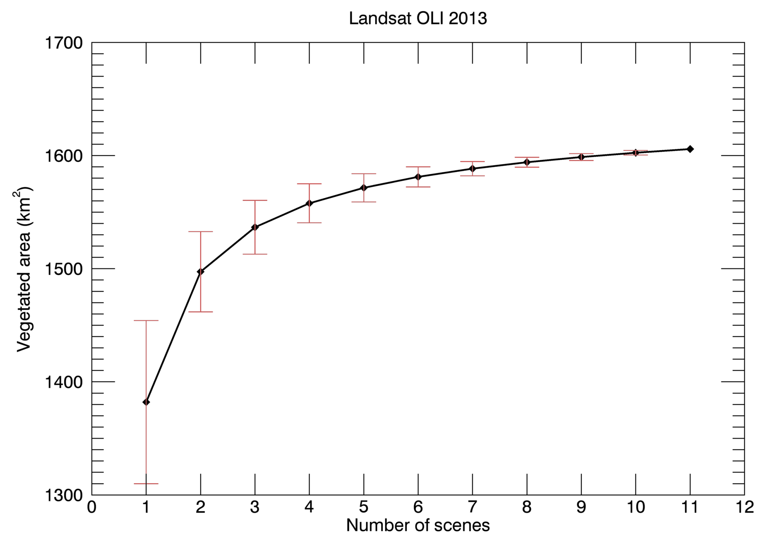
• assessing the improvements in the detection of cultivated areas which can be obtained using a number of images to produce the classification for a specific year.

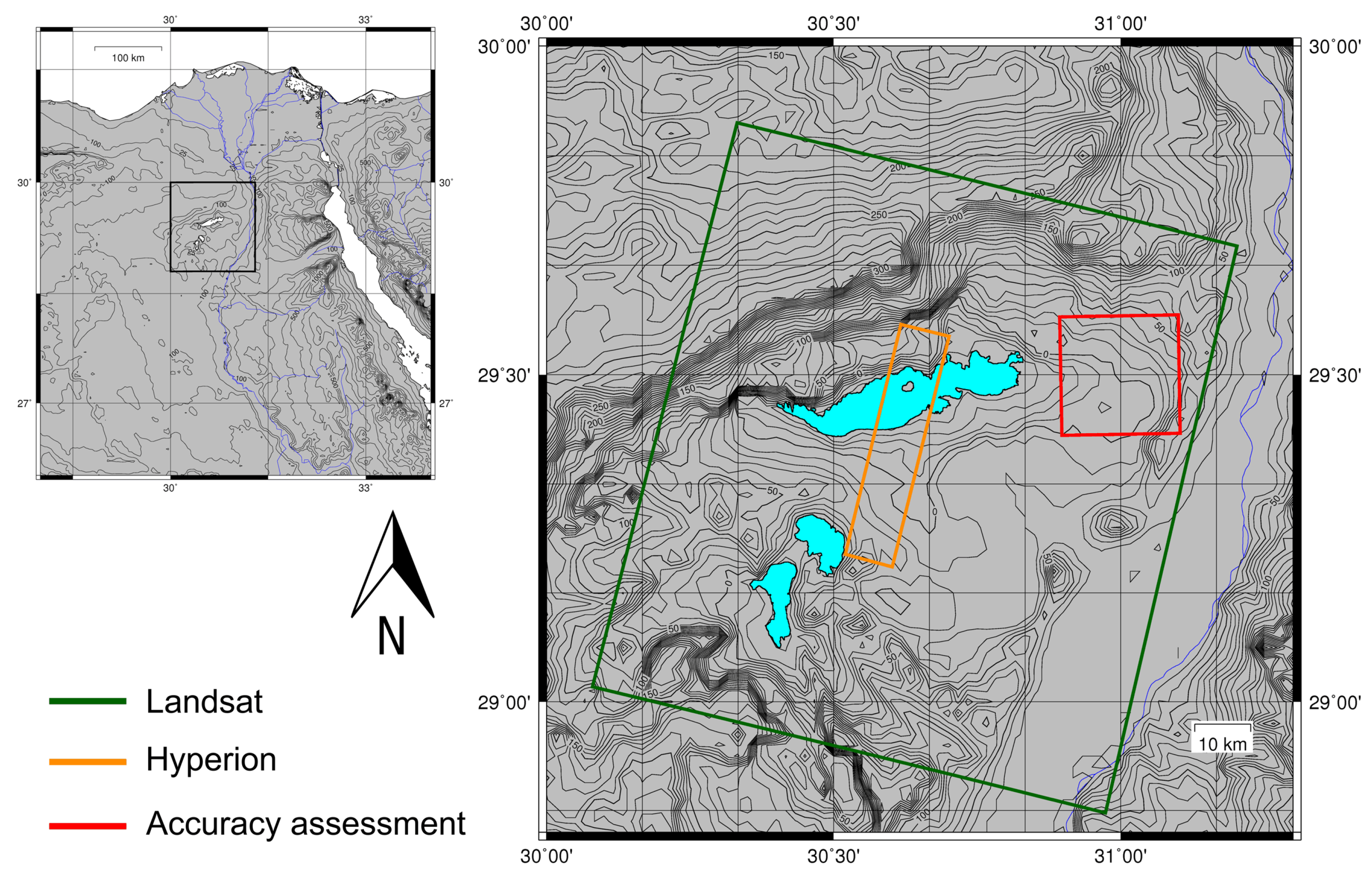
The change detection was carried out on a set of Landsat images from 1987 to 2013, while the cross-comparison analysis among the sensors of the Landsat series was performed on the basis of simulated data, generated from a hyperspectral Hyperion image.

2. Study Area

The Fayyum depression is one of the most productive agricultural regions of Egypt and has been since ancient times. For this reason it is often designated in literature as Fayyum Oasis. The first systematic reclamation of the area dates back to the XIX century B.C., under the Pharaohs of the XII dynasty. Nowadays, over 2.5 million people live in the oasis with a mean population density of 1400 people per km². The oasis and surrounding desert also have a wealth of natural and cultural heritage sites [11]. To ensure a sustainable use of these resources, the Fayyum Oasis and, in particular, Lake Qarun were designated as a conservation area in 1989.

The oasis occupies a topographically depressed area, located about 90 km south-west of Cairo [12]. The northern and deepest part of the depression is covered by Lake Qarun, which extends for about 240 km². To the south and east, the lake is surrounded by agricultural land, whose elevation ranges from about 40 m below sea level to about 30 m above. The main crops are cereals (maize, wheat, sorghum and rice), vegetables, fruit, cotton and livestock fodder. Only 20% of the cultivations are perennial and the cropping intensity (the total cropped area divided by the physical area) is 190%, which means that there are two cycles a year for many crops [13].

The typical Saharan climate of the area, with scarce precipitations (less than 10 mm/year) and very high evaporation potential, has a strong control over the ecosystem [14,15]. The water needs of the oasis are entirely supplied by fresh Nile water, which is distributed around the cultivated fields through a network of canals. Discharge waters are collected into Lake Qarun and partly into the adjacent Wadi El-Rayan depression [16]. This hydrological setting and the increasing human pressure, as a consequence of the expansion in cultivation, have been causing land degradation and deterioration in lake water quality (in particular, salinisation and eutrophication [17,18]). Recent studies indicate that 54% of cultivated soils are affected by a severe risk of chemical degradation, due to climatic, pedological and topographical factors, and 65% are subject to improper land management and irrigation practices, heightening the actual risk [19].

3. Materials

3.1. Hyperspectral Data

Hyperspectral data were used to simulate a consistent set of images of the Landsat series (covering the same area at the same time) and to evaluate the impact on the change detection process of the radiometric differences among the Landsat sensors.

One image from the Hyperion sensor (installed onboard the Earth Observing 1 platform) was acquired on 15 December 2009. It covers a narrow portion (7.5 km wide) of the western part of the Fayyum Oasis (Figure 1). Hyperion is a pushbroom sensor which provides 242 bands, continuously covering the visible and near infrared portion of the spectrum, between 0.4 and 2.5 micrometers, with a spectral resolution of approximately 10 nm [20].

Figure 1. Location of the study area and data coverage.

Figure 1. Location of the study area and data coverage.

3.2. Landsat Data

The dataset for the change detection study consists of 56 multispectral Landsat 5 TM, Landsat 7 ETM and Landsat 8 OLI frames, belonging to rows 39 and 40 of path 177. The time steps to be investigated were chosen from years with at least five cloud- and haze-free scenes (representative for all seasons) available in the Landsat archive (Table 1). The minimum of five images is a compromise between data availability and desirable accuracy, as discussed in Section 6. In all, twelve frames were collected from 1987, ten from 1998 (plus two from February 1999 to compensate for a lack of winter images in 1998), ten from 2003 and 20 from 2013 (plus two from January 2014, also in this case to compensate for a lack of winter images).

Table 1. Satellite images from the Landsat archive used for the change detection analysis.

	Jan	Feb	Mar	Apr	May	Jun	Jul	Aug	Sep	Oct	Nov	Dec
1987	TM	TM		TM		TM	TM		TM
1998				TM	TM			TM		TM		TM
1999		TM
2003	ETM				ETM	TM		TM		TM
2013			OLI		OLI	OLI	OLI	OLI	OLI		OLI	OLI
2014	OLI

Table 1. Satellite images from the Landsat archive used for the change detection analysis.

	Jan	Feb	Mar	Apr	May	Jun	Jul	Aug	Sep	Oct	Nov	Dec
1987	TM	TM		TM		TM	TM		TM
1998				TM	TM			TM		TM		TM
1999		TM
2003	ETM				ETM	TM		TM		TM
2013			OLI		OLI	OLI	OLI	OLI	OLI		OLI	OLI
2014	OLI

3.3. High Resolution Data

As stated by Hecheltjen et al. [7], “accuracy assessment remains a challenge in change extraction analyses, principally due to the limited availability of complete timely in situ ground information”. Usually, when good quality control points verified on the ground are not available, the land cover map is compared with some higher quality information source [21].

In order to provide the reference data for 2013 land cover, several images from the Google Earth platform were used, acquired between April and December of the same year. For 2003, only few images acquired between October 2002 and February 2003 were available and only the eastern part of the oasis was covered. For this reason, the accuracy assessment was limited to a 20 by 20 km area, located in the north-eastern border of the oasis, which is believed to be representative of the major dynamics occurring in the region. This area, in fact, is one of the most affected by the reclamation process taking place over the last two decades, and one of the most prone to salinisation and calcicity-related degradation [22].

4. Methods

4.1. Landsat Sensor Comparison

The change detection study presented in Section 4.2 made use of three Landsat sensors (TM, ETM and OLI), therefore it is useful to assess to what extent the different radiometric characteristics of the sensors can affect the computation of vegetation index values.

The most relevant differences can be found in the behaviour of the relative spectral response functions (RSRFs) and in the number of quantisation levels. The near-infrared band of the OLI sensor is by far narrower than the corresponding TM and ETM bands (the bandwidth of OLI band 5 is about 30 nm, while ETM band 4 is 130 nm). Furthermore, OLI images are quantised in 12 bits instead of the 8 bits of its predecessors.

In order to evaluate the effects of these differences, a set of Landsat images (TM, ETM, OLI) covering the same area was generated performing a spectral convolution on the Hyperion image.

It is well known that hyperspectral images require more complex calibration procedures to retrieve accurate radiance values, because of their lower signal to noise ratio, the strong correlation between contiguous bands and some artefacts, like smiling and streaking or outlier pixels [23]. In the present study, the calibration were performed by a set of software applications developed by CSIRO (Australian Commonwealth Scientific and Industrial Research Organisation) [24]. The most sensitive step in this phase is de-streaking, the removal of a vertical line pattern caused by a distinctive push-broom sensor along-track effect.

Starting from the calibrated radiance values, two image cubes were computed: the top of atmosphere (TOA) reflectance image and the surface reflectance (SR) image. The former was obtained by dividing the spectral radiance by the solar irradiance (assuming a lambertian behaviour), whilst the latter required an atmospheric correction model. For this study, the atmospheric correction was performed using the Visual SixS software package [25], which is an implementation of the 6SV radiative transfer code.

Spectral convolutions were performed on the two hyperspectral image cubes to simulate multispectral images acquired by TM, ETM and OLI sensors. Both TOA and surface reflectances were considered. SR values simulated from the atmospheric corrected hyperspectral image are useful to evaluate the radiometric differences among the corresponding bands of the different Landsat sensors, in particular the near infrared (NIR) ones. In this way, it is also possible to quantify the impact of these differences in the normalised difference vegetation index (NDVI) values.

On the other hand, TOA reflectance values allow to simulate the effectiveness of the invariant object correction method [26] in accommodating both atmospheric effects and inconsistencies due to the radiometry of the different sensors. SR signatures of a few selected pixels were extracted from the simulated TM image; these signatures were used as reference to calculate the OLI surface reflectance starting from the simulated OLI TOA reflectance. In fact, this procedure reproduces the normalisation technique used in the change detection analyses presented in Section 4.2.

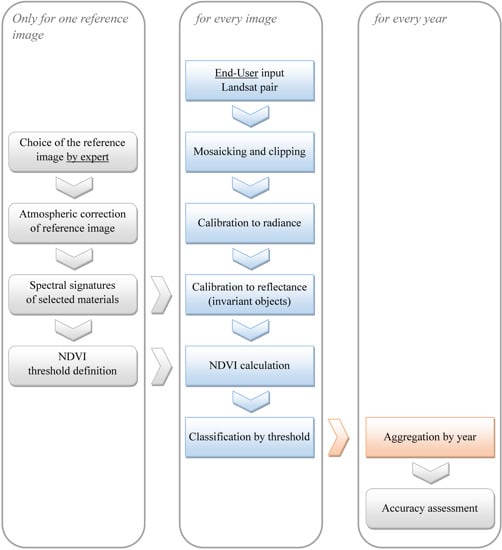
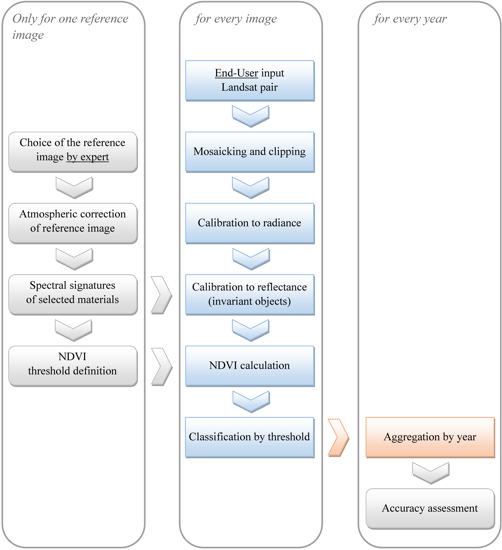
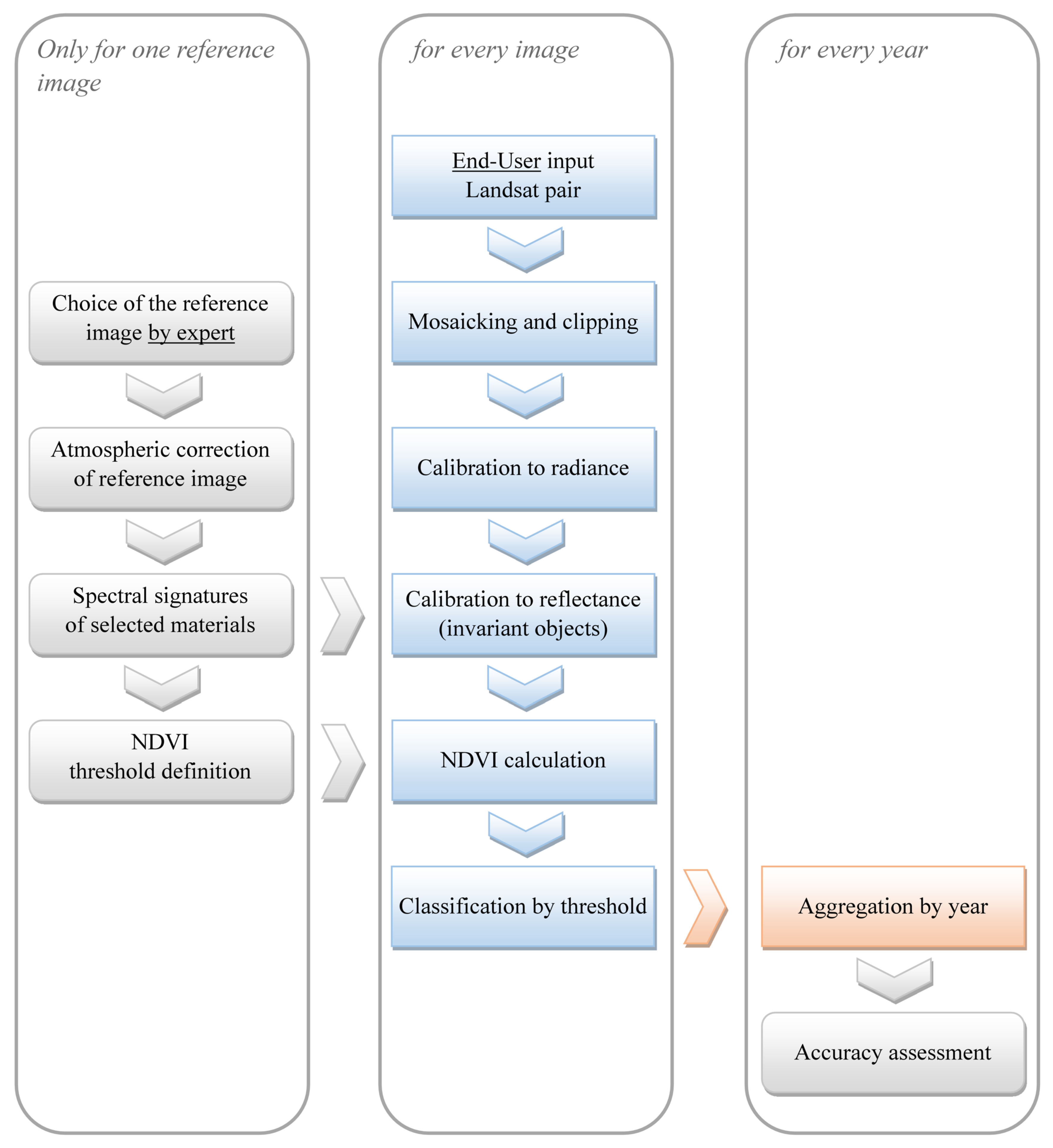
4.2. Change Detection

This section describes the work carried out at regional level to quantify the expansion of cultivated land over the past decades, implementing a new automated software tool for this purpose. As mentioned in Section 2, a wide variety of crops are cultivated in the study area, both perennial and seasonal. Here, however, the only aim is to measure the total extension of the cultivated fields, regardless the crop types.

In order to achieve the desired level of automation, a hybrid method was proposed, based on the computation of a vegetation index and a classification process. All the images collected from the Landsat archive were therefore classified into “vegetated” or “non vegetated” areas; the classification is carried out by calculating the NDVI (on SR values) and defining a threshold.

To process the entire dataset, a fully automated procedure was implemented in ENVI-IDL. Once set up, the batch programme is designed in such a way that the final user need only select the images to be processed and the classified map is generated in output.

The procedure involves several steps (Figure 2). Firstly, mosaicking is carried out for the two Landsat frames covering the entire oasis (about 2880 km²), for each acquisition date. However, before the vegetation index was computed, several pre-processing operations were implemented, as the entire time series had to be as homogeneous and coherent as possible, in terms of both geometry and radiometry. Clearly, all the images must be spatially co-registered to avoid detecting spurious changes. The data set consists only of geometrically corrected L1T products, which are coherent with each other (with an accuracy of less than one pixel), all being orthorectified using the same data (i.e., GLS2000) [27].

In addition, if a unique threshold is adopted for all images, each must be calibrated and corrected for atmospheric effects, at least in a relative way. To address this issue, the TM image acquired on 28 June 2003 was chosen as the reference scene, with respect to the remainder of the series. This is the only image that was pre-processed manually to apply the appropriate atmospheric correction using the 6SV radiative transfer code [28]. The required input parameters were derived from MODIS Terra atmospheric products.

All the other images were calibrated automatically using the invariant object method [26]. The spectral signatures of a few selected rock outcrops (i.e., basalt or limestone) were extracted from the previously corrected reference image; these surfaces are assumed to be spectrally invariant over time. Each image was then normalised to the reference image using a linear regression based on these invariant objects.

Figure 2. Block diagram outlining the main processing steps implemented in the automated procedure.

Figure 2. Block diagram outlining the main processing steps implemented in the automated procedure.

A threshold on the NDVI value was established for the reference image ($NDVI>0.25$) on the basis of image statistics and with the aid of photo-interpretation. The criteria followed are illustrated in Figure 3. A few samples of bare soil, urban and vegetated areas (covering 0.45, 0.90 and 0.93 km² respectively) were identified by photo-interpretation. The histogram of NDVI values for these three categories were analyzed to define the threshold. The main problem here is represented by the overlap between vegetation and urban land covers. For example, given the distributions of Figure 3, the critical NDVI value of 0.25 is approximately “equidistant” from the means of the two distributions (about 1.7 times its standard deviation); according to Chebyshev’s inequality, the probability of classifying a “vegetated” pixel correctly is greater than 68%, whereas the probability of wrongly including an “urban” pixel in the vegetation class is lower than 19%.

Figure 3. Histograms of NDVI for bare soil, urban and vegetated land cover samples, identified through photo-interpretation. The overlap between distributions of vegetation and urban land covers is illustrated.

Figure 3. Histograms of NDVI for bare soil, urban and vegetated land cover samples, identified through photo-interpretation. The overlap between distributions of vegetation and urban land covers is illustrated.

The NDVI value was then computed on each single image (see Figure 4) and the predefined threshold applied to distinguish the vegetated areas. In the light of the outcomes of the cross-comparison analysis described in Section 5.1, the threshold value was adjusted to 0.26 for Landsat 8 images, according to the equation of the regression line showed in Figure 5f.

Finally, the representative classification for a specific year was produced on a per-pixel basis by counting the number of Landsat images acquired in that year where the pixel was classified as “vegetated”. For example, the pixel defined as cultivated in Figure 4 was classified as vegetated in the images acquired in April, August and December 1998 and as non-vegetated in those acquired in May and October of the same year; this means that it belongs to “Class 3” in the 1998 combined classification, since it was classified three-times as vegetated.

4.3. Accuracy Assessment

The assessment of the accuracy of the maps produced was carried out by photo-interpretation using high resolution imagery. The assessment was not performed on the single-image maps but only on the aggregated classifications. In particular, two years were evaluated, 2003 and 2013. The accuracy was evaluated also for the change detection between these two years.

Change, in general, is a rare event [29], in the sense that only a limited number of pixels in the scene are actually affected by change. Thus, to assess the accuracy of a change detection map, a stratified sampling design is to be implemented in order to prioritise sampling in areas where change occurred and avoid accuracy overestimation. The zone, in which the accuracy assessment was performed, was therefore divided in two strata. The first stratum is defined by comparing the classifications of 2003 and 2013 and it contains the pixels where a change in land cover was detected. The second stratum contains all the remaining pixels.

Figure 4. NDVI time series of two pixels (see Figure 6 for location). The first (green circles) belongs to a field under cultivation since 1987, while the second (blue diamonds) belongs to land reclaimed in 2011. The continuous grey line indicates the threshold of the NDVI value.

Figure 4. NDVI time series of two pixels (see Figure 6 for location). The first (green circles) belongs to a field under cultivation since 1987, while the second (blue diamonds) belongs to land reclaimed in 2011. The continuous grey line indicates the threshold of the NDVI value.

In the “no change” stratum 116 points were selected on a regular grid according to systematic sampling strategy, since it achieves the criterion of spatial balance [21]. The grid spacing was set to 2 km. In the “change” stratum, instead, 50 check points were randomly selected, since a systematic sampling was not feasible due to the limited extent of the stratum. Two points were discarded, because it was impossible to determine their major land cover type (considering the 30 m pixel size of Landsat images). The land cover was assessed through photo-interpretation of the high resolution images provided by Google Earth. The visual interpretation, here, reproduced the classification process, so points interpreted as cultivated in at least one high resolution image are assigned to the vegetated reference data. However, plots of land which appear ploughed are considered cultivated even if a green cover is not present.

The confusion matrices presented in Section 5.2 were expressed in terms of proportion of areas, according to the following expression:

$$p_{ij}={\displaystyle \frac{1}{N}}\sum _{k=1}^K{\displaystyle \frac{N_k}{n_k}}{n}_{ijk}$$

(1)

where $p_{ij}$ is the proportion of area classified in the i-th class and belonging to the j-th class according to the reference data, N is the total pixel population, K is the number of strata, $N_k$ is the number of pixels of the population belonging to the k-th stratum, $n_k$ is the number of pixels of the sample belonging to the k-th stratum and $n_{ijk}$ is the number of pixels in the sample belonging to the k-th stratum, classified in the i-th class but belonging to the j-th class according to the reference data.

Figure 5. NDVI scatter plots to compare the sensors of the Landsat series, based on simulations through one Hyperion image. (a), (b) comparison between NDVI values (TM vs. ETM and OLI respectively) computed from reflectances derived by 6SV model and convolved; (c), (d) NDVI values from TM image corrected by 6SV (assumed as reference) vs. values from simulated ETM and OLI images respectively, corrected by invariant object (IO) method; (e), (f) the same as (c), (d) but for a narrower wavelength interval (0.24–0.26 microns). Regression lines are plotted in red colour, identity lines in black.

Figure 5. NDVI scatter plots to compare the sensors of the Landsat series, based on simulations through one Hyperion image. (a), (b) comparison between NDVI values (TM vs. ETM and OLI respectively) computed from reflectances derived by 6SV model and convolved; (c), (d) NDVI values from TM image corrected by 6SV (assumed as reference) vs. values from simulated ETM and OLI images respectively, corrected by invariant object (IO) method; (e), (f) the same as (c), (d) but for a narrower wavelength interval (0.24–0.26 microns). Regression lines are plotted in red colour, identity lines in black.

It must be noted here that Equation (1) is different from the usual formula for the stratified sampling design (cf. [30]), because in this case the strata are not coincident with the classes. Its derivation, however, follows the general definition of an unbiased linear estimator of the population total from a sample, which makes use of the inclusion probability, i.e., the a priori probability that a generic element will be included in a sample of a given size [31].

Besides the commonly adopted parameters, such as the overall accuracy and the omission and commission errors, the “quantity disagreement” and the “allocation disagreement” proposed by Pontius Jr and Millones [32] were also computed.

5. Results

5.1. Landsat Sensor Comparison

The NDVI images obtained from the spectral convolutions described in Section 4.1 were compared (Figure 5), analysing scatter plots and computing regression lines. In the perspective of change detection analyses, the following outcomes are relevant:

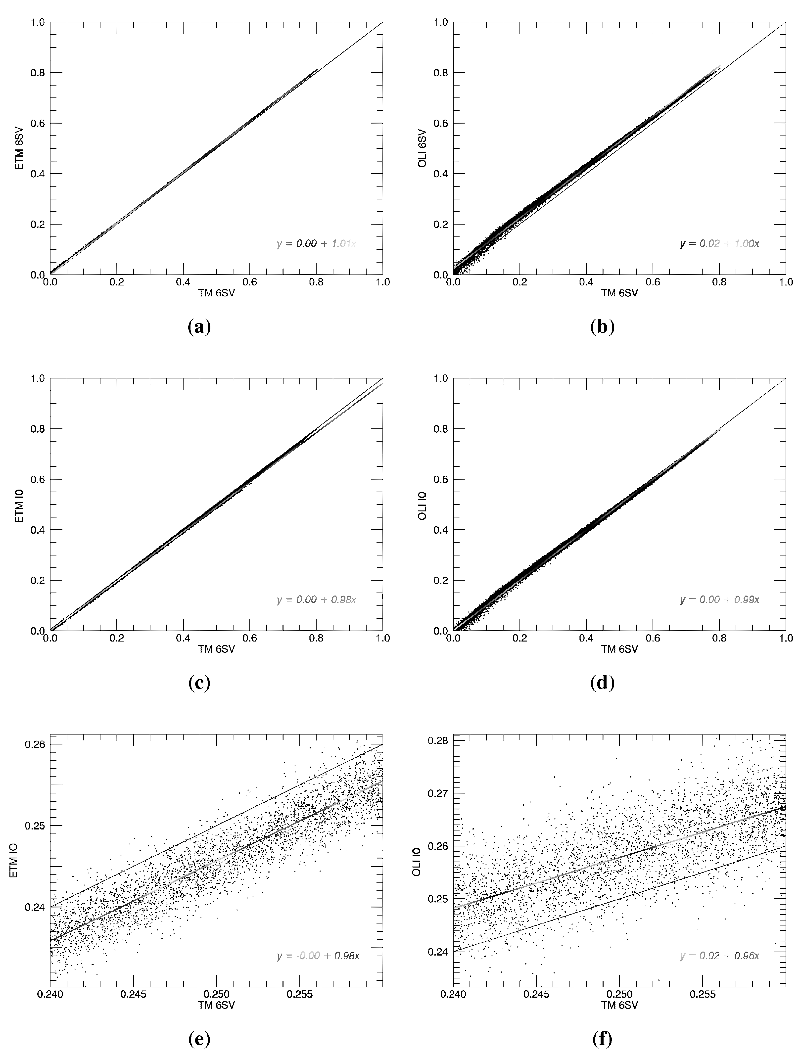
• Considering the behaviour of the NDVI within the interval between zero and one, the correlation between the simulated TM and ETM values is very high and the regression line of the scatter plot is quite coincident with the identity line (Figure 5a). This means that the spectral differences between the NIR and red bands of the two sensors are negligible for a large number of practical applications.
• The linear correlation between simulated TM and OLI values is still high (Figure 5b), even if lower than the one between TM and ETM. However, the intercept of the regression line was found to be about 0.02. The plot appears more scattered, therefore, if an interval of NDVI values in the TM domain is selected, the corresponding interval of values in the OLI domain will be broader. In this case, spectral differences can affect significantly applications which exploit vegetation indexes.
• The use of the invariant object method to perform the relative atmospheric correction of a OLI image, assuming a TM image as reference, seems to accommodate the global bias due to the different radiometry of the two sensors (Figure 5d). However, if the correlation is evaluated within a narrower interval (Figure 5f), the regression line diverges significantly from the identity line. This result may be relevant for processing chains involving thresholds, suggesting that threshold values need to be adjusted, when moving from TM to OLI images.

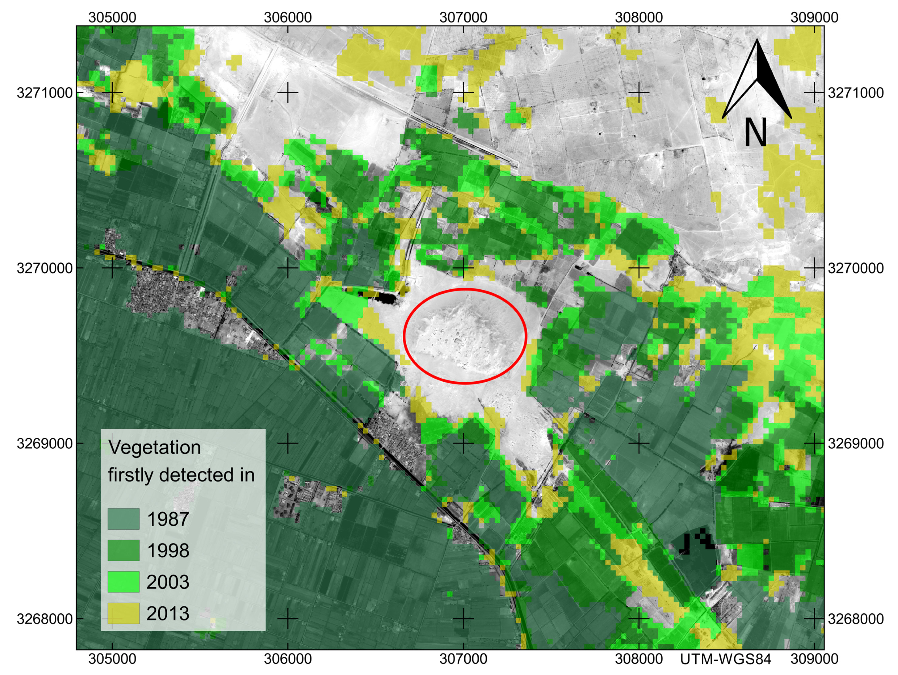
5.2. Change Detection

By analysing the results of the whole classification process on the entire Landsat time series, summarised in Table 2, it is possible to outline the expansion of the cultivated area in the Fayyum Oasis since 1987. The total increase is estimated to be approximately 89 km² (101 considering solution 2013b) and the greatest increment occurred between 2003 and 2013. The major expansion areas are located close to the borders of the oasis, while some areas changed from vegetated to non-vegetated especially around towns and villages, likely as a consequence of the urban growth.

The statistics in Figure 6, which relate to the areas classified as vegetated in the five Landsat images taken in 2003, show that only 49% of the pixels were identified as vegetated in all the five images and only 27% in at least four scenes. The total area under cultivation estimated in the 2003 aggregate classification is 1528 km². Using a single date classification, the result would be underestimated, and the cultivated area would be at its minimum in May (only 1047 km²) and maximum in January (1471 km²).

Table 2. Extension of the cultivated fields in the four years under examination and areal percentage of each class (the class number indicates how many times the pixel was classified as vegetated during the same year). For 2013, the first solution made use of six images only (March, May, June, August, November, January), solution “b” of all the images available.

Year	Total Area	Class 1	Class 2	Class 3	Class 4	Class 5	Class 6 or Higher
	km2	%	%	%	%	%	%
1987	1500	3	4	7	12	27	47
1998	1504	5	5	11	22	41	16
2003	1528	5	6	13	27	49	-
2013	1589	3	3	5	7	17	65
2013b	1601	2	2	2	2	2	90

Table 2. Extension of the cultivated fields in the four years under examination and areal percentage of each class (the class number indicates how many times the pixel was classified as vegetated during the same year). For 2013, the first solution made use of six images only (March, May, June, August, November, January), solution “b” of all the images available.

Year	Total Area	Class 1	Class 2	Class 3	Class 4	Class 5	Class 6 or Higher
	km2	%	%	%	%	%	%
1987	1500	3	4	7	12	27	47
1998	1504	5	5	11	22	41	16
2003	1528	5	6	13	27	49	-
2013	1589	3	3	5	7	17	65
2013b	1601	2	2	2	2	2	90

Figure 6. Aggregated classification of the 2003 Landsat series. The series is composed of ten images acquired on five different dates. All the coloured pixels are classified as vegetated and the class number indicates how many times the pixel has been classified as vegetated. The pie-chart shows the areal percentage of each class. The red polygon delimits the area where the accuracy assessment was performed. The red circle and the diamond indicate the positions of the two pixels of Figure 4.

Figure 6. Aggregated classification of the 2003 Landsat series. The series is composed of ten images acquired on five different dates. All the coloured pixels are classified as vegetated and the class number indicates how many times the pixel has been classified as vegetated. The pie-chart shows the areal percentage of each class. The red polygon delimits the area where the accuracy assessment was performed. The red circle and the diamond indicate the positions of the two pixels of Figure 4.

In 2013 the situation appears different, thanks to the higher number of images available (22 images for 11 dates). The first solution in Table 2 is obtained using only six images (March, May, June, August, November, January), resembling the timing of previous years. The second solution (labelled 2013b, using all the images) counts 11 classes and 57% of vegetated pixels belongs to Class 11, while 15% to Class 10. The difference in cultivated area between the two solutions is about 0.8%. In Figure 7 a portion of the change detection map located in the accuracy assessment area is shown.

Figure 7. Change detection map of the area around the archaeological site of Bakchias (marked by a red circle), located in the accuracy assessment area. The areas in darkest green colour designate the fields detected as vegetated in the oldest image of the dataset (1987).

Figure 7. Change detection map of the area around the archaeological site of Bakchias (marked by a red circle), located in the accuracy assessment area. The areas in darkest green colour designate the fields detected as vegetated in the oldest image of the dataset (1987).

5.3. Accuracy Assessment

The confusion matrix of the aggregated classification of 2003 is reported in Table 3a, in terms of proportions of the area in which the assessment was performed. The overall accuracy equals to 94% and the disagreement can be decomposed in a quantity disagreement by 4% and an allocation disagreement by 2%. Omission error amounts to 8% for vegetated surfaces and to 3% for non-vegetated ones, whilst commission errors amount to 2% and 11% respectively.

The overall accuracy of the 2013 aggregated classification (Table 3b, solution with six images) is almost the same, 95%. In this case the total quantity disagreement decreases to 1%, whereas the allocation one raises to 4%. Omission error decreases to 5% for vegetated surfaces and raises to 5% for non-vegetated ones. Commission errors amount to 4% and 7% respectively.

In Table 4 the confusion matrix for the change detection between 2003 and 2013 classifications is reported. The first two by two block corresponds to the “no-change” part of the matrix. The overall accuracy, here, is 91%, which is slightly better than the product of the accuracy values for the two classifications. The total quantity disagreement is 4%, while the allocation one is 5%.

Closely examining the change class “Non-vegetated to Vegetated”, the specific quantity disagreement is 3%, however, omission and commission errors are 24% and 53% respectively. Two types of commission errors are present in this change class: the first is due to the growth of spontaneous vegetation along canal banks or near ponds, the second to the inclusion of urban pixels, especially in rural villages. Instead, the most frequent omission errors are related to crops with very low vegetation cover.

Table 3. Confusion matrices for the (a) 2003 and (b) 2013 classifications. “V” stands for “Vegetated” surfaces, whilst “N” for “Non vegetated”. Matrices are expressed in terms of proportions of area.

(a) 2003

	V	N
V	0.5362	0.0105	0.55
N	0.0483	0.4050	0.45
	0.58	0.42	1.00

(a) 2003

	V	N
V	0.5362	0.0105	0.55
N	0.0483	0.4050	0.45
	0.58	0.42	1.00

(b) 2013

	V	N
V	0.5572	0.0223	0.58
N	0.0280	0.3925	0.42
	0.59	0.41	1.00

(b) 2013

	V	N
V	0.5572	0.0223	0.58
N	0.0280	0.3925	0.42
	0.59	0.41	1.00

Table 4. Confusion matrix for the change detection between 2003 and 2013 classifications. “V” stands for “Vegetated” surfaces, whilst “N” for “Non vegetated”, so, for example, “NV” means a change from Non-vegetated in 2003 to Vegetated in 2013.

	VV	NN	VN	NV
VV	0.5057	0.0081	0.0012	0.0000	0.52
NN	0.0093	0.3527	0.0175	0.0093	0.39
VN	0.0093	0.0024	0.0199	0.0000	0.03
NV	0.0215	0.0130	0.0000	0.0300	0.06
	0.55	0.38	0.04	0.04	1.00

Table 4. Confusion matrix for the change detection between 2003 and 2013 classifications. “V” stands for “Vegetated” surfaces, whilst “N” for “Non vegetated”, so, for example, “NV” means a change from Non-vegetated in 2003 to Vegetated in 2013.

	VV	NN	VN	NV
VV	0.5057	0.0081	0.0012	0.0000	0.52
NN	0.0093	0.3527	0.0175	0.0093	0.39
VN	0.0093	0.0024	0.0199	0.0000	0.03
NV	0.0215	0.0130	0.0000	0.0300	0.06
	0.55	0.38	0.04	0.04	1.00

6. Discussion

In Egypt, change detection studies were conducted recently in areas of intense reclamation [33,34]. In essence, they were based on the analysis of full land cover maps, obtained by supervised classification of images acquired in different years. These classifications, however, were enhanced by visual interpretation to improve the final accuracy. A further study by Hereher [35] over the whole country used coarse resolution MODIS AQUA imagery and Enhanced Vegetation Index to estimate the increment of vegetated area between 2003 and 2012 (more than 4200 km²). In all these works, the land cover change between two years was assessed by comparing two single-date images, adopting a “bi-temporal” approach.

The processing of the Landsat time series presented in this paper clearly highlights the effects of seasonal harvesting cycles and the importance of working with many images for each year being studied. This challenge was investigated by Pax Lenney et al. [36] in a work assessing the status of agricultural lands in some areas in the Nile Delta, using ten Landsat TM images dating from 1984 to 1993. They found that classification methods based on multitemporal NDVI features (i.e., statistics describing trends), were successful in distinguishing healthy cultivated lands from non-productive lands and to identify reclaimed areas. They found also that high-frequency multitemporal data sets are needed to monitor agricultural landscapes, especially where agricultural practices result in great temporal variability. The results presented in Section 5.2 of the present paper confirm the findings by Pax Lenney and Woodcock [37], who observed an underestimation ranging between 4% and 42%, using only one image. These facts appear to be a consequence of the wide variety of crops grown in the study area within a flexible cropping schedule. Also a recent study by Knudby et al. [38] demonstrates that building one supervised classification from multiple images can improve overall accuracy and fill eventual gaps in the coverage.

The availability of a large number of OLI images in 2013 (11 dates) allowed the execution of some tests to evaluate the variation of the area detected as vegetated as a function of the number of images used. The vegetated area was estimated using all the possible combinations of one, two, three, etc. images. For example, using only one image there are eleven estimates of the area since there are eleven images, instead, using five images (of eleven) there are 462 possible combinations and so 462 estimates. The means and standard deviations are plotted in Figure 8. The mean value grows monotonically but asymptotically with the number of images. The choice of selecting at least five images for each year is clearly a compromise between accuracy and limited availability of images of the earlier Landsat missions. It should be noted, however, that the choice should be restricted to those combinations which includes all the seasons. With this restriction, the area detected as vegetated using five images decreases by 1.5% in average in respect of using all eleven images. A problem is the detection of short period crops. For example, the reclaimed pixel in Figure 4 exceeded the threshold for no more than two months consecutively. In this case, an acquisition frequency lower than one image every two months would not ensure the detection and could lead to a lower accuracy.

Therefore, two solutions were presented in Table 2 for 2013. The first made use of six images, chosen to resemble the situation encountered in the previous years examined. The second solution (2013b) made use of all the eleven images available and represents a situation which is going to be common thanks to the high acquisition rate of Landsat 8 and the availability of Sentinel-2 imagery (especially considering the forthcoming launch of Sentinel-2b). The difference in area was found to be about 0.8%, which means a difference of 12% in the estimate of the cultivation expansion between 1987 and 2013. Differences in overall accuracy, instead, were found to be negligible, considering the given set of check points.

Regarding the processing chain, the critical point that most affects the results is defining the threshold for the NDVI. In general, as noted by Lu et al. [8], the choice of threshold is highly subjective and scene-dependent, and it is often set either through a trial-and-error procedure or using statistical measures. In particular, setting a static threshold (based on the reference Landsat image) may lead to either an overestimation or an underestimation of the vegetation cover, especially if a single image classification only is considered. However, working in a context involving a wide variety of crops (each with its specific phenological phases) and high cropping intensity, this effect can be minimised by using multiple images acquired during different seasons. On the other hand, a varying threshold would compromise one of the main goals, that is, the high level of automation of the monitoring procedure.

Figure 8. Variation of the area detected as vegetated as a function of the number of images used, considering all the possible combinations of the eleven OLI images available for 2013. Whiskers refer to the standard deviation.

Figure 8. Variation of the area detected as vegetated as a function of the number of images used, considering all the possible combinations of the eleven OLI images available for 2013. Whiskers refer to the standard deviation.

It is important to point out also that the threshold should be adjusted when moving from TM to OLI data, because the differences in radiometry between the two sensors affects the values of the NDVI. This adjustment, however, can be quantified a priori and implemented in the processing chain. The same considerations apply also when using ETM and OLI sensors together. The differences in NDVI values observed in the simulations performed on hyperspectral Hyperion data (Section 5.1) are of the same magnitude of those reported by Li et al. [3], but in this case the simulated NDVI values from OLI are systematically greater than the ones from TM.

Although validation is still not possible because of the lack of a statistically significant amount of ground truth data over the entire oasis, the accuracy of the classifications on the last two years considered was assessed using high resolution images. The error matrices were not compiled for the classifications of every single image but only for the aggregated classifications representative for the two years. The idea behind this choice is that, independently of the day when the high resolution image was acquired, if a reference site is seen to be cultivated on that specific day, the assumption is that it must be classified as vegetated in the aggregate classification, since this provides a representation of the entire year. Conversely, it is theoretically possible that some uncultivated reference sites are cultivated in subsequent months; in this case, false errors would be introduced to the confusion matrix.

The overall accuracies achieved confirm the feasibility of the proposed method. On the one hand, the decrease of the quantity disagreement in 2013 classification suggests that the higher number of images used (eleven dates instead of five) improved the detection process, as can be seen also from the decrease of the omission error of Vegetated class. On the other hand, errors due to mixed pixels accumulate as the number of images used increases. This effect is highlighted by the raise of the omission error for Non-vegetated class and of the total allocation error. The problem of mixed pixels is exacerbated in Landsat imagery because of the cubic convolution resampling algorithm applied to all Landsat data to perform the orthorectification. Omission errors for Non-vegetated class can be related also to the relatively high NDVI values observed in urban areas, especially in rural villages.

The use of different sensors for the change detection introduces further errors; in particular, as described in Section 5.1, the tests carried out on simulated data show that NDVI values derived from OLI images are more scattered than the corresponding values derived from TM or ETM images, especially close to the threshold value. This fact contributes to the large commission error observed in the specific change category from Non-vegetated to Vegetated.

Among the possible vegetation indexes, NDVI was chosen for the present study to carry out the classification into “vegetated” versus “non-vegetated” categories. Other indexes based on the soil line, such as SAVI, were also tested; however, despite providing better results in the case of very low vegetation density, they produce more confusion in urban areas and consequently a slightly lower overall accuracy. A possible indicator which may be implemented in future developments of the algorithm is greenness, since it can take into account more bands than only the red and NIR ones [39].

The solution presented here was designed in order to take into account the characteristic environment of the Fayyum Oasis, where cultivated fields are surrounded only by desert soils and there is hardly any spontaneous vegetation. It should be noted, however, that the reclamation of desert areas through artificial irrigation is a common practice for developing countries in arid climatic zones; this means that interest in a specialised monitoring strategy is fully justified. The procedure described has, indeed, the advantage of being easy to repeat and may be suitable for long-term monitoring over wide areas where systematic and repeated field surveying is not feasible.

7. Conclusions

This work presents an efficient methodology for long-term monitoring of the expansion of cultivation in arid environments, using three sensors of the Landsat series (TM, ETM, and the new OLI) and taking into account their differences in radiometry. The methodology was tested in the Fayyum Oasis (Egypt). A surface of 2880 km² at four time steps were investigated (years 1987, 1998, 2003 and 2013); the total increase of cultivated areas was estimated to be between 89 and 101 km². A full change error matrix was compiled in order to assess the accuracy of the change detection between the last two years considered.

The hybrid change detection approach, which combines the computation of the NDVI index with a classification into “vegetated” or “non vegetated” areas, offers the advantage of concentrating all discretionary assumptions during the initial setting-up stage, allowing for the full automation of the procedure.

One distinctive aspect is the use of multiple images to produce a single classification that is representative of an entire year. This proved to be essential for the following reasons: (1) it mitigates errors due to seasonal harvesting cycles (which can lead to underestimating the cultivated surface significantly, sometimes in excess of 30%); (2) it increases the robustness of the solution obtained using a specific threshold (overall accuracy up to 90% for change detection), because the final decision does not rely on a single observation.

The methodology proposed here was designed for arid landscapes and this can limit its areas of application. However, this solution can be applied to other regions with similar characteristics, which are not uncommon in arid climates, and it can work even if good quality training data are not available. Furthermore, it can be easily applied to the new Sentinel-2 imagery [40], after an appropriate cross-comparison analysis is conducted.

References

1. Irons, J.R.; Dwyer, J.L.; Barsi, J.A. The next Landsat satellite: The Landsat data continuity mission. Remote Sens. Environ. 2012, 122, 11–21. [Google Scholar] [CrossRef]
2. Roy, D.; Wulder, M.; Loveland, T.; Woodcock, C.; Allen, R.; Anderson, M.; Helder, D.; Irons, J.; Johnson, D.; Kennedy, R.; et al. Landsat-8: Science and product vision for terrestrial global change research. Remote Sens. Environ. 2014, 145, 154–172. [Google Scholar] [CrossRef]
3. Li, P.; Jiang, L.; Feng, Z. Cross-comparison of vegetation indices derived from Landsat-7 Enhanced Thematic Mapper Plus (ETM+) and Landsat-8 Operational Land Imager (OLI) sensors. Remote Sens. 2014, 6, 310–329. [Google Scholar] [CrossRef]
4. Singh, A. Digital change detection techniques using remotely-sensed data. Int. J. Remote Sens. 1989, 10, 989–1003. [Google Scholar] [CrossRef]
5. Canty, M.J. Image Analysis, Classification, and Change Detection in Remote Sensing: With Algorithms for ENVI/IDL, 2nd ed.; CRC Press: Boca Raton, FL, USA, 2010. [Google Scholar]
6. Almutairi, A.; Warner, T.A. Change Detection Accuracy and Image Properties: A Study Using Simulated Data. Remote Sens. 2010, 2, 1508–1529. [Google Scholar] [CrossRef]
7. Hecheltjen, A.; Thonfeld, F.; Menz, G. Recent advances in remote sensing change detection—A review. In Land Use and Land Cover Mapping in Europe; Manakos, I., Braun, M., Eds.; Springer Netherlands: Dordrecht, The Netherlands, 2014; pp. 145–178. [Google Scholar]
8. Lu, D.; Mausel, P.; Brondízio, E.; Moran, E. Change detection techniques. Int. J. Remote Sens. 2004, 25, 2365–2401. [Google Scholar] [CrossRef]
9. Coppin, P.; Jonckheere, I.; Nackaerts, K.; Muys, B.; Lambin, E. Review ArticleDigital change detection methods in ecosystem monitoring: A review. Int. J. Remote Sens. 2004, 25, 1565–1596. [Google Scholar] [CrossRef]
10. Hobbs, R.J. Remote sensing of spatial and temporal dynamics of vegetation. In Remote Sensing of Biosphere Functioning; Hobbs, R.J., Mooney, H.A., Eds.; Springer: New York, NY, USA, 1990; pp. 203–219. [Google Scholar]
11. Ramzy, Y.H. Sustainable tourism development in Al Fayoum Oasis, Egypt. In Ecosystem and Sustainable Development IX; Marinov, A.M., Brebbia, C.A., Eds.; WIT Press: England, UK, 2013; pp. 164–173. [Google Scholar]
12. Bitelli, G.; Curzi, P.V.; Mandanici, E. Morphological and lithological aspects in the northeastern Libyan desert by remote sensing. Proc. SPIE 2009. [Google Scholar] [CrossRef]
13. Khattab, A.F.; Abdel Azim, R.; El Masry, S. Water Trading in Fayoum and Frafra Oasis; Technical Report 72; United States Agency for International Development: Cairo, Egypt, 2003.
14. Ishak, M.M.; Abdel Malek, S.A. Some ecological aspects of lake Qarun, Fayoum, Egypt. Part I: Physico-chemical environment. Hydrobiologia 1980, 74, 173–178. [Google Scholar] [CrossRef]
15. El Shabrawy, G.M.; Dumont, H.J. The Fayum depression and its lakes. In The Nile. Origin, Environments, Limnology and Human Use; Dumont, H.J., Ed.; Springer: New York, NY, USA, 2009; pp. 95–124. [Google Scholar]
16. Hereher, M.E. Assessing the dynamics of El-Rayan lakes, Egypt, using remote sensing techniques. Arab. J. Geosci. 2015, 8, 1931–1938. [Google Scholar] [CrossRef]
17. Hussein, H.; Amer, R.; Gaballah, A.; Refaat, Y.; Abdel-Wahab, A. Polluton monitoring for Lake Qarun. Adv. Environ. Biol. 2008, 2, 70–80. [Google Scholar]
18. Bitelli, G.; Curzi, P.V.; Dinelli, E.; Mandanici, E. Empirical model for salinity assessment on lacustrine and coastal waters by remote sensing. Proc. SPIE 2011. [Google Scholar] [CrossRef]
19. Ali, R.R.; Abdel Kawy, W.A.M. Land degradation risk assessment of El Fayoum depression, Egypt. Arab. J. Geosci. 2013, 6, 2767–2776. [Google Scholar] [CrossRef]
20. Ungar, S.G.; Pearlman, J.S.; Mendenhall, J.A.; Reuter, D. Overview of the Earth Observing One (EO-1) Mission. IEEE Trans. Geosci. Remote Sens. 2003, 41, 1149–1159. [Google Scholar] [CrossRef]
21. Stehman, S.V. Sampling designs for accuracy assessment of land cover. Int. J. Remote Sens. 2009, 30, 5243–5272. [Google Scholar] [CrossRef]
22. Abd Elgawad, M.; Shendi, M.M.; Sofi, D.M.; Abdurrahman, H.A.; Ahmed, A.M. Geographical Distribution of Soil Salinity, Alkalinity, and Calcicity Within Fayoum and Tamia Districts, Fayoum Governorate, Egypt. In Developments in Soil Salinity Assessment and Reclamation; Shahid, S.A., Abdelfattah, M.A., Taha, F.K., Eds.; Springer: Dordrecht, The Netherlands, 2013; pp. 219–236. [Google Scholar]
23. Liao, L.B.; Jarecke, P.J.; Gleichauf, D.A.; Hedman, T.R. Performance characterization of the Hyperion Imaging Spectrometer instrument. SPIE Proc. 2000, 4135, 264–275. [Google Scholar]
24. Jupp, D.L.B.; Datt, B. Evaluation of Hyperion Performance at Australian Hyperspectral Calibration and Validation Sites; Technical Report; CSIRO Earth Observation Centre Report: Canberra, Australia, 2004. [Google Scholar]
25. Mandanici, E. Implementation of Hyperion sensor routine in 6SV radiative transfer code. In Proceedings of the Hyperspectral Workshop 2010, Frascati, Italy, 17–19 March 2010.
26. Liang, S. Quantitative Remote Sensing of Land Surfaces; John Wiley & Sons: Hoboken, NJ, USA, 2004. [Google Scholar]
27. Gutman, G.; Byrnes, R.; Masek, J.; Covington, S.; Justice, C.; Franks, S.; Headley, R. Towards Monitoring Land-Cover and Land-Use Changes at a Global Scale: The Global Land Survey 2005. Photogr. Eng. Remote Sens. 2008, 74, 6–10. [Google Scholar]
28. Kotchenova, S.Y.; Vermote, E.F.; Matarrese, R.; Klemm, Frank J., Jr. Validation of a vector version of the 6S radiative transfer code for atmospheric correction of satellite data. Part I: Path radiance. Appl. Opt. 2006, 45, 6762–6774. [Google Scholar] [CrossRef] [PubMed]
29. Congalton, R.G.; Green, K. Assessing the Accuracy of Remotely Sensed Data: Principles and Practices; CRC Press: Boca Raton, FL, USA, 2002. [Google Scholar]
30. Stehman, S.V.; Czaplewski, R.L. Design and Analysis for Thematic Map Accuracy Assessment: Fundamental Principles. Remote Sens. Environ. 1998, 64, 331–344. [Google Scholar] [CrossRef]
31. Särndal, C.E.; Swensson, B.; Wretman, J. Model Assisted Survey Sampling; Springer: Berlin, Germany, 1992. [Google Scholar]
32. Pontius, R.G., Jr.; Millones, M. Death to Kappa: birth of quantity disagreement and allocation disagreement for accuracy assessment. Int. J. Remote Sens. 2011, 32, 4407–4429. [Google Scholar] [CrossRef]
33. Shalaby, A.; Tateishi, R. Remote sensing and GIS for mapping and monitoring land cover and land-use changes in the Northwestern coastal zone of Egypt. Appl. Geogr. 2007, 27, 28–41. [Google Scholar] [CrossRef]
34. El Kawy, O.R.A.; Rød, J.K.; Ismail, H.A.; Suliman, A.S. Land use and land cover change detection in the western Nile delta of Egypt using remote sensing data. Appl. Geogr. 2011, 31, 483–494. [Google Scholar] [CrossRef]
35. Hereher, M.E. The status of Egypt’s agricultural lands using MODIS Aqua data. Egypt. J. Remote Sens. Space Sci. 2013, 16, 83–89. [Google Scholar] [CrossRef]
36. Pax Lenney, M.; Woodcock, C.E.; Collins, J.B.; Hamdi, H. The status of agricultural lands in Egypt: The use of multitemporal NDVI features derived from landsat TM. Remote Sens. Environ. 1996, 56, 8–20. [Google Scholar] [CrossRef]
37. Pax Lenney, M.; Woodcock, C.E. Monitoring agricultural lands in Egypt with multitemporal Landsat TM imagery: How many images are needed? Remote Sens. Environ. 1997, 59, 522–529. [Google Scholar] [CrossRef]
38. Knudby, A.; Nordlund, L.M.; Palmqvist, G.; Wikström, K.; Koliji, A.; Lindborg, R.; Gullström, M. Using multiple Landsat scenes in an ensemble classifier reduces classification error in a stable nearshore environment. Int. J. Appl. Earth Observ. Geoinf. 2014, 28, 90–101. [Google Scholar] [CrossRef]
39. Zanchetta, A.; Bitelli, G.; Karnieli, A. Tasselled Cap transform for change detection in the drylands: Findings for SPOT and Landsat satellites with FOSS tools. Proc. SPIE 2015. [Google Scholar] [CrossRef]
40. Drusch, M.; del Bello, U.; Carlier, S.; Colin, O.; Fernandez, V.; Gascon, F.; Hoersch, B.; Isola, C.; Laberinti, P.; Martimort, P.; et al. Sentinel-2: ESA’s optical high-resolution mission for GMES operational services. Remote Sens. Environ. 2012, 120, 25–36. [Google Scholar] [CrossRef]