
Modeling Microwave Emission from Short Vegetation-Covered Surfaces


Abstract
:
1. Introduction
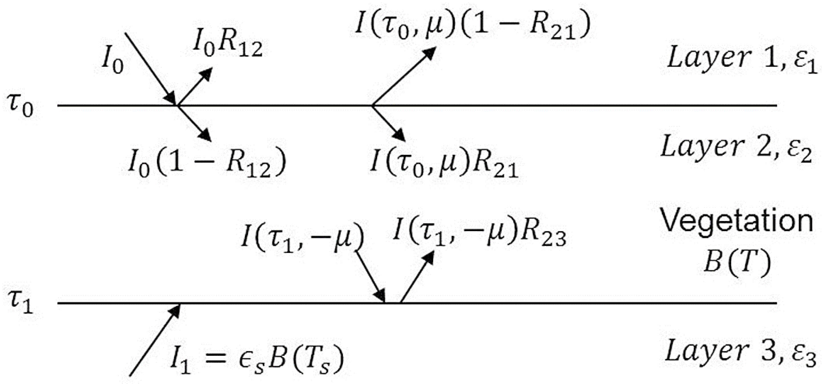
2. Methodology

2.1. Vegetation Volume Scattering
2.1.1. The Geometric Optics Approach for Leaves
2.1.2. Infinite Cylinder Approximation for Stems
- ,
- ,
- ,
- ,
- ,
- ,
- ,
- ,
- ,
- ,
- ,
- ,
- ,
- .
2.1.3. Vegetation Optic Parameters
2.2. Rough Surface Reflection
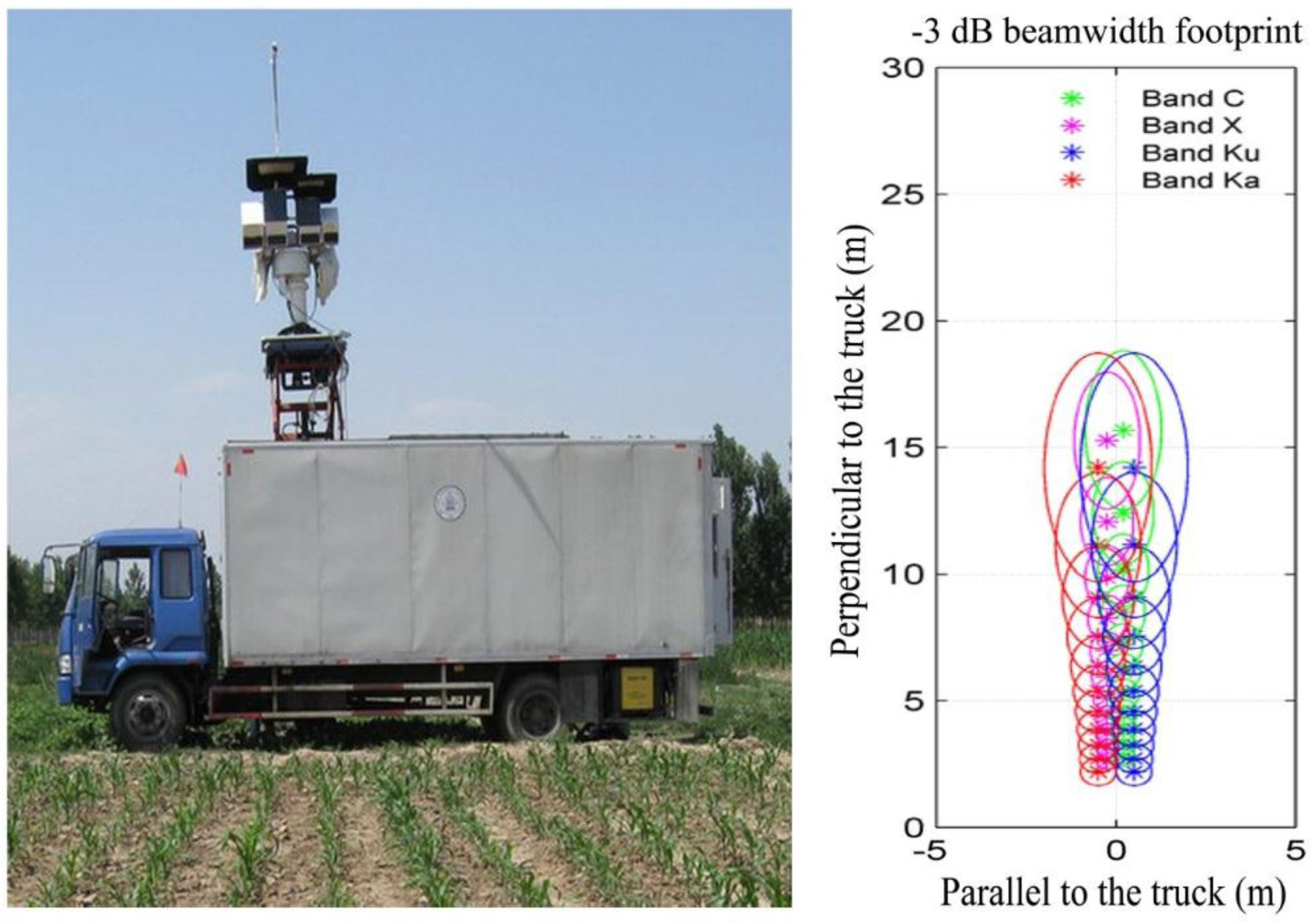
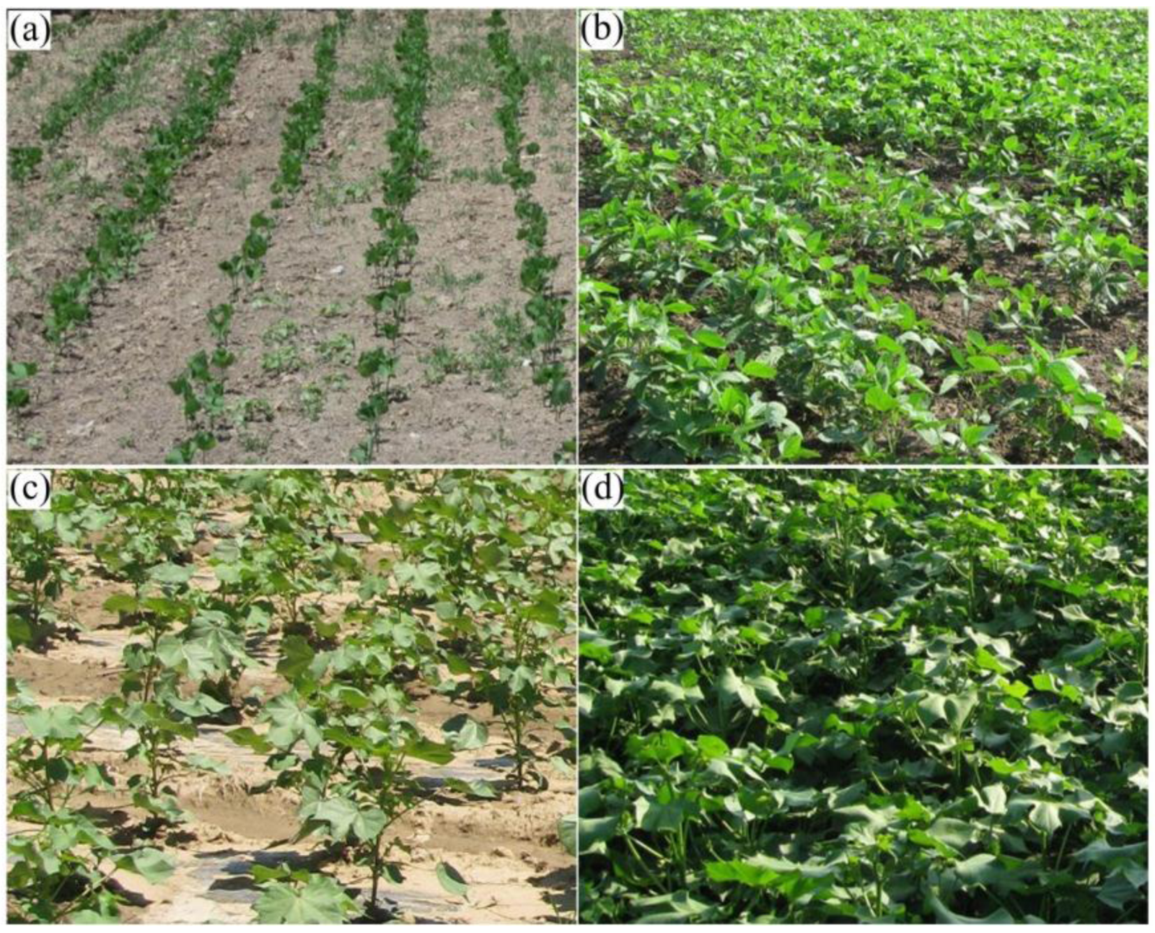
3. Field Experimental Data


| Scatterers | Measured Parameters | Soybean | Cotton | ||
|---|---|---|---|---|---|
| 23 June | 9 July | 10 June | 23 June | ||
| Vegetation | Depth (m) | 0.11 | 0.33 | 0.19 | 0.37 |
| Temperature (°C) | 36.8 | 29.4 | 26.3 | 29.4 | |
| Leaves | LAI (m2∙m−2) | 0.58 | 1.35 | 0.71 | 1.57 |
| Thickness (mm) | 0.31 | 0.38 | 0.23 | 0.27 | |
| Mg (g∙g−1) | 0.85 | 0.75 | 0.82 | 0.80 | |
| Stems | Radius (m) | 0.0009 | 0.0013 | 0.0026 | 0.003 |
| Length (m) | 0.05 | 0.08 | 0.08 | 0.15 | |
| Mg (g∙g−1) | 0.88 | 0.82 | 0.88 | 0.90 | |
| Density (m−2) | 277 | 378 | 285 | 327 | |
| Angle distribution | oblique | oblique | oblique | oblique | |
| Rough soil surface | SMC (cm3∙cm−3) | 0.0138 | 0.162 | 0.30 | 0.05 |
| RMS height (m) | 0.03 | 0.03 | 0.02 | 0.03 | |
| Correlation length (m) | 0.09 | 0.09 | 0.1 | 0.1 | |
| Skin temperature (°C) | 49.5 | 33.2 | 34.5 | 42.1 | |
| Soil temperature (°C) | 43.1 | 32.9 | 31.5 | 33.6 | |
4. Results and Discussion
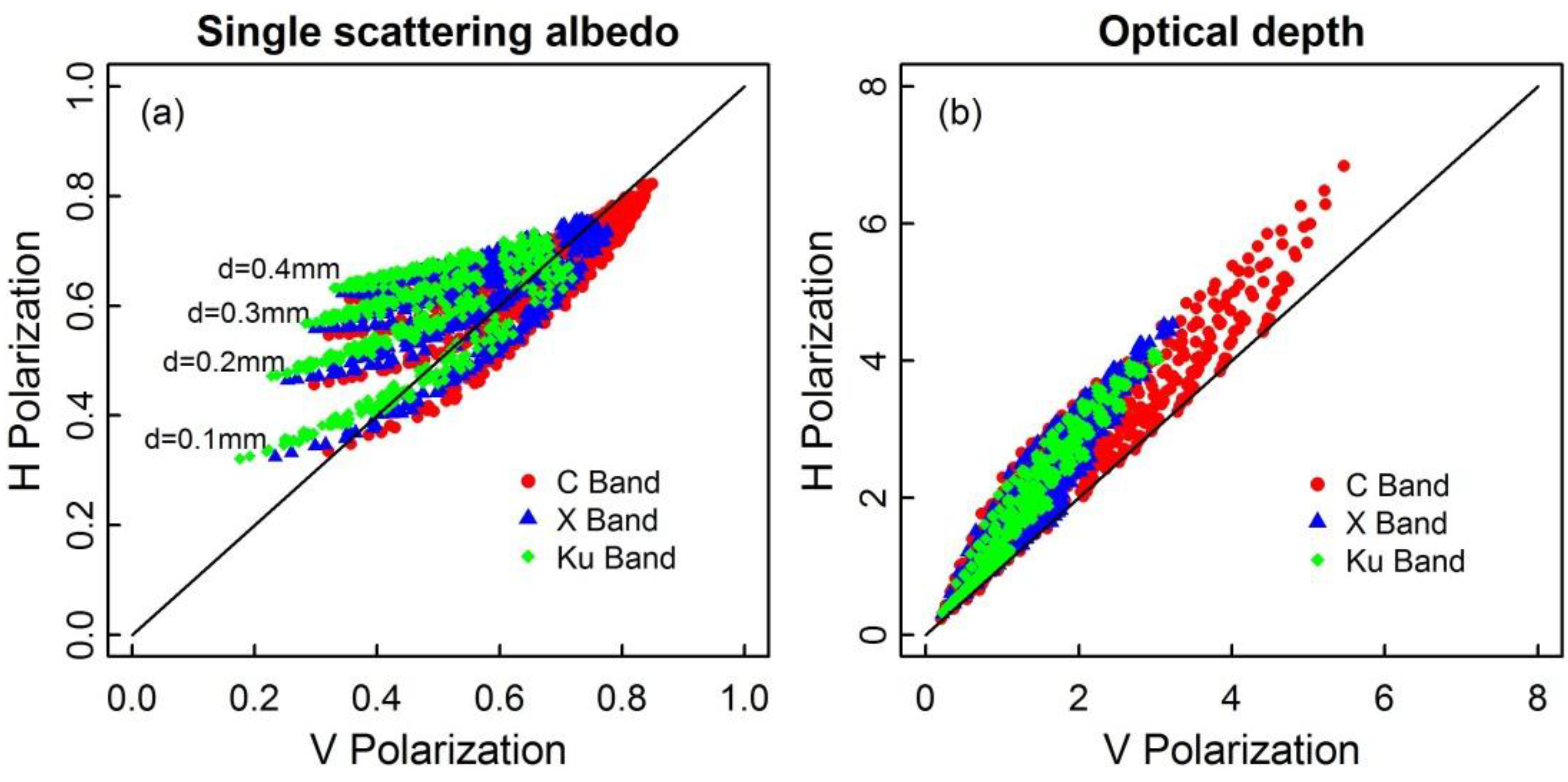
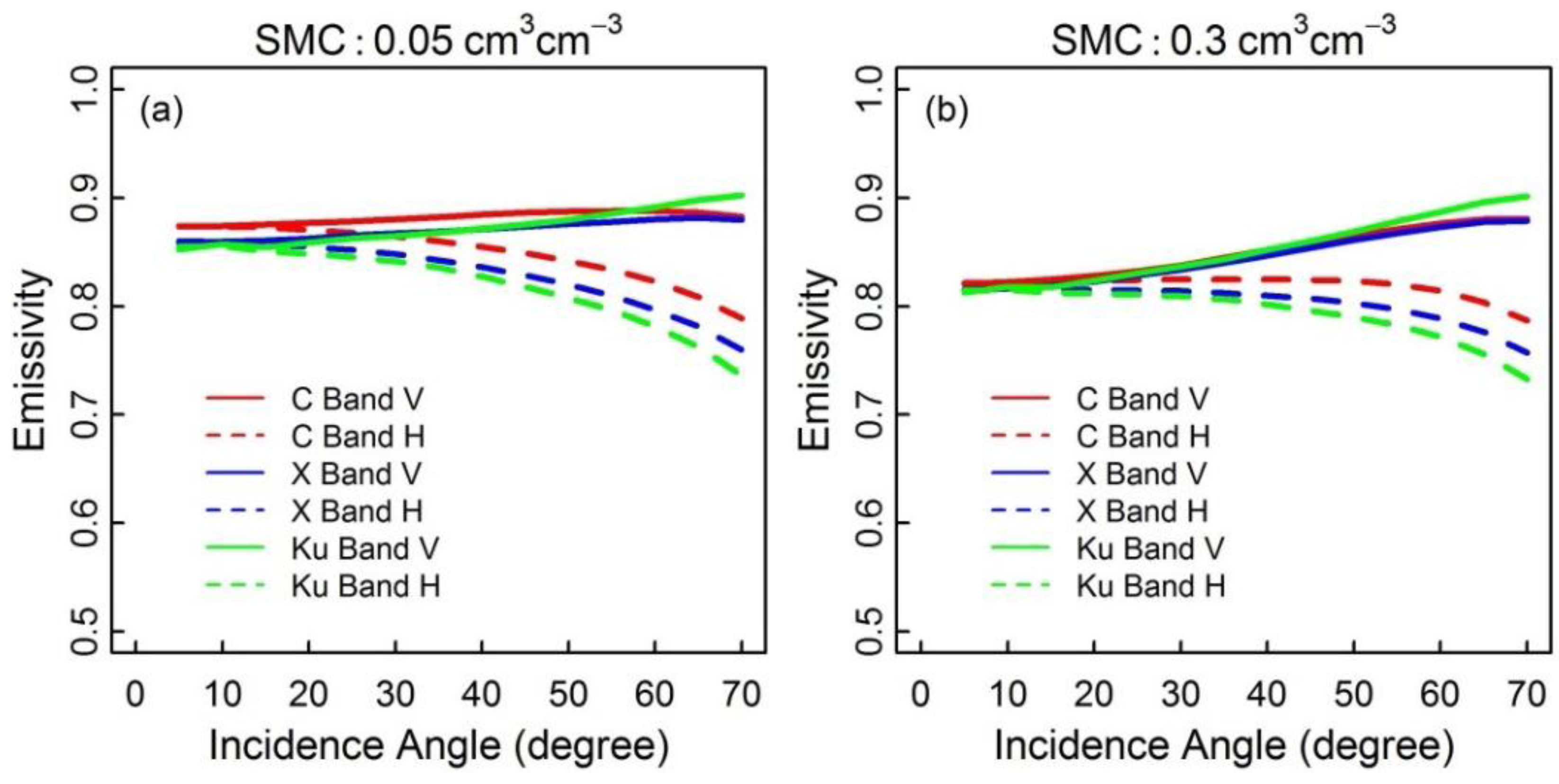
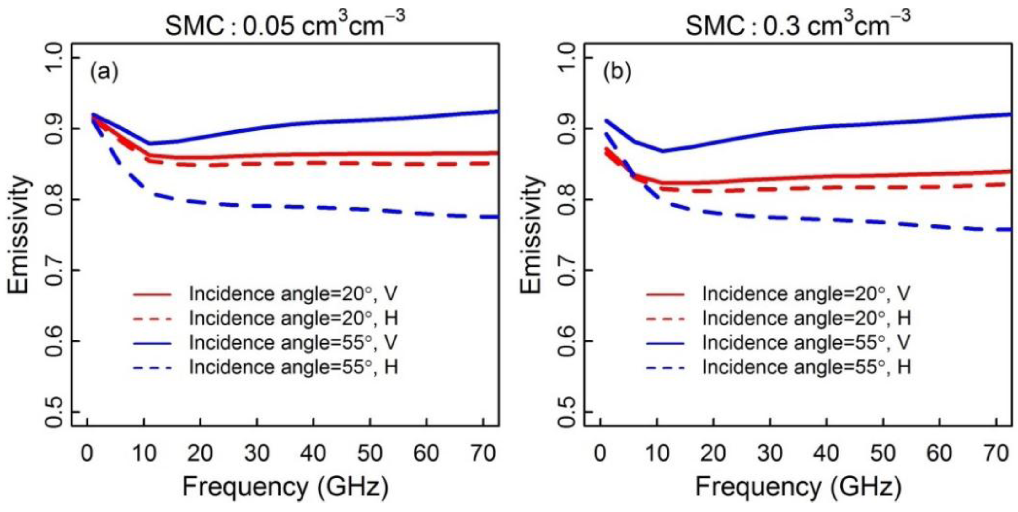
4.1. Parameters Sensitivity
| Scatterers | Parameters | Minimum | Maximum | Interval | Number |
|---|---|---|---|---|---|
| Leaves | LAI (m2∙m−2) | 0.5 | 5.5 | 1.0 | 6 |
| Thickness (mm) | 0.1 | 0.4 | 0.1 | 4 | |
| Mg (g g−1) | 0.60 | 0.80 | 0.10 | 3 | |
| Stems | Radius (m) | 0.002 | 0.022 | 0.004 | 6 |
| Height (m) | 0.2 | 1.0 | 0.2 | 5 | |
| Mg (g∙g−1) | 0.50 | 0.70 | 0.10 | 3 | |
| Density (m−2) | 50 | 200 | 50 | 4 |


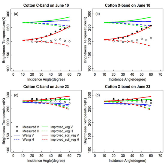
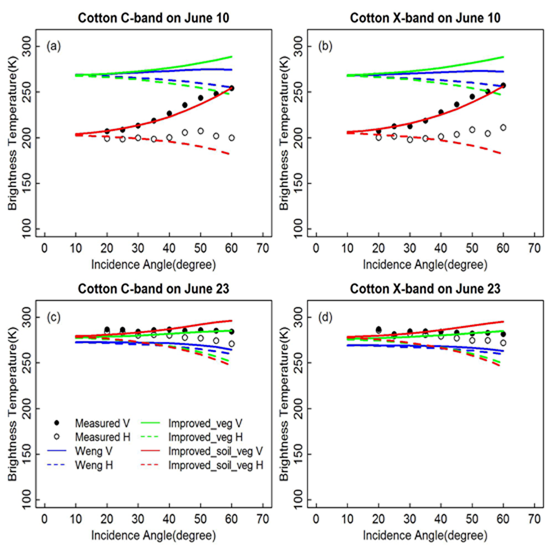
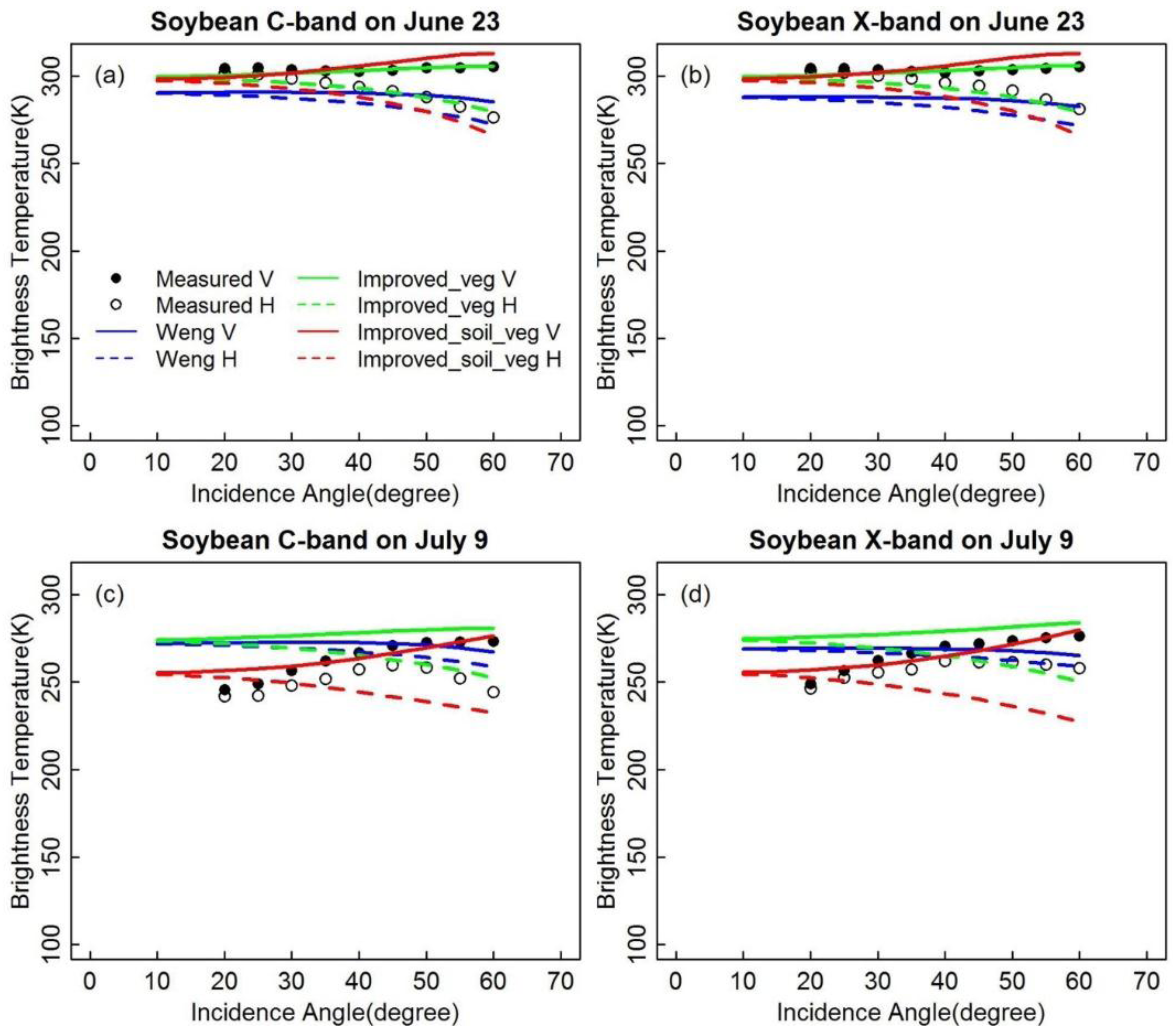
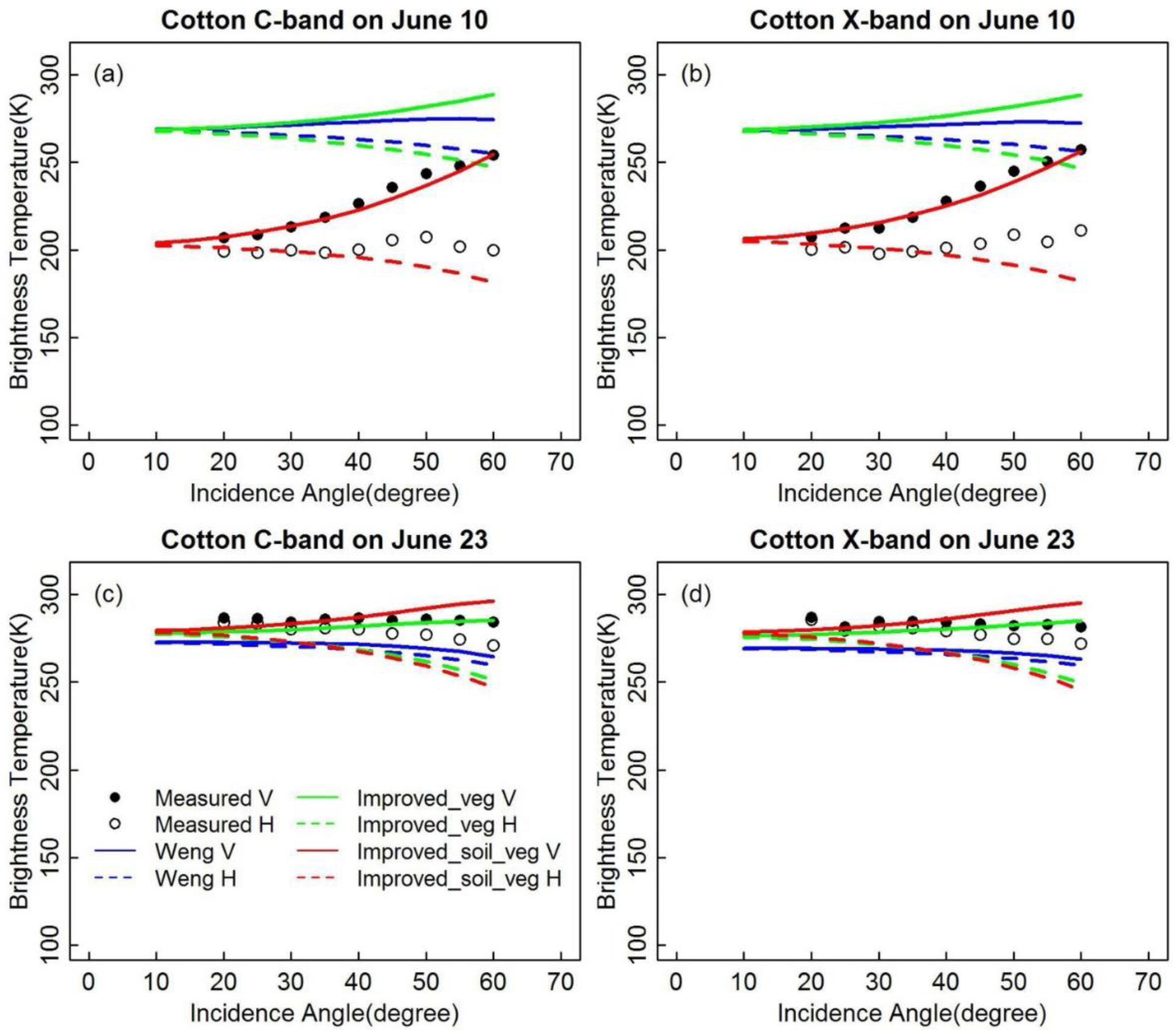
4.2. Comparisons with Field Experimental Data


| Models | Weng Model | Improved_veg | Improved_soil_veg | ||||
|---|---|---|---|---|---|---|---|
| Statistics | C Band | X Band | C Band | X Band | C Band | X Band | |
| R2 | V | 0.33 | 0.27 | 0.62 | 0.60 | 0.98 | 0.97 |
| H | 0.50 | 0.42 | 0.49 | 0.44 | 0.95 | 0.93 | |
| RMSE | V | 26.67 | 25.70 | 26.71 | 25.71 | 5.03 | 5.19 |
| H | 32.81 | 31.77 | 30.86 | 29.67 | 11.73 | 14.92 | |
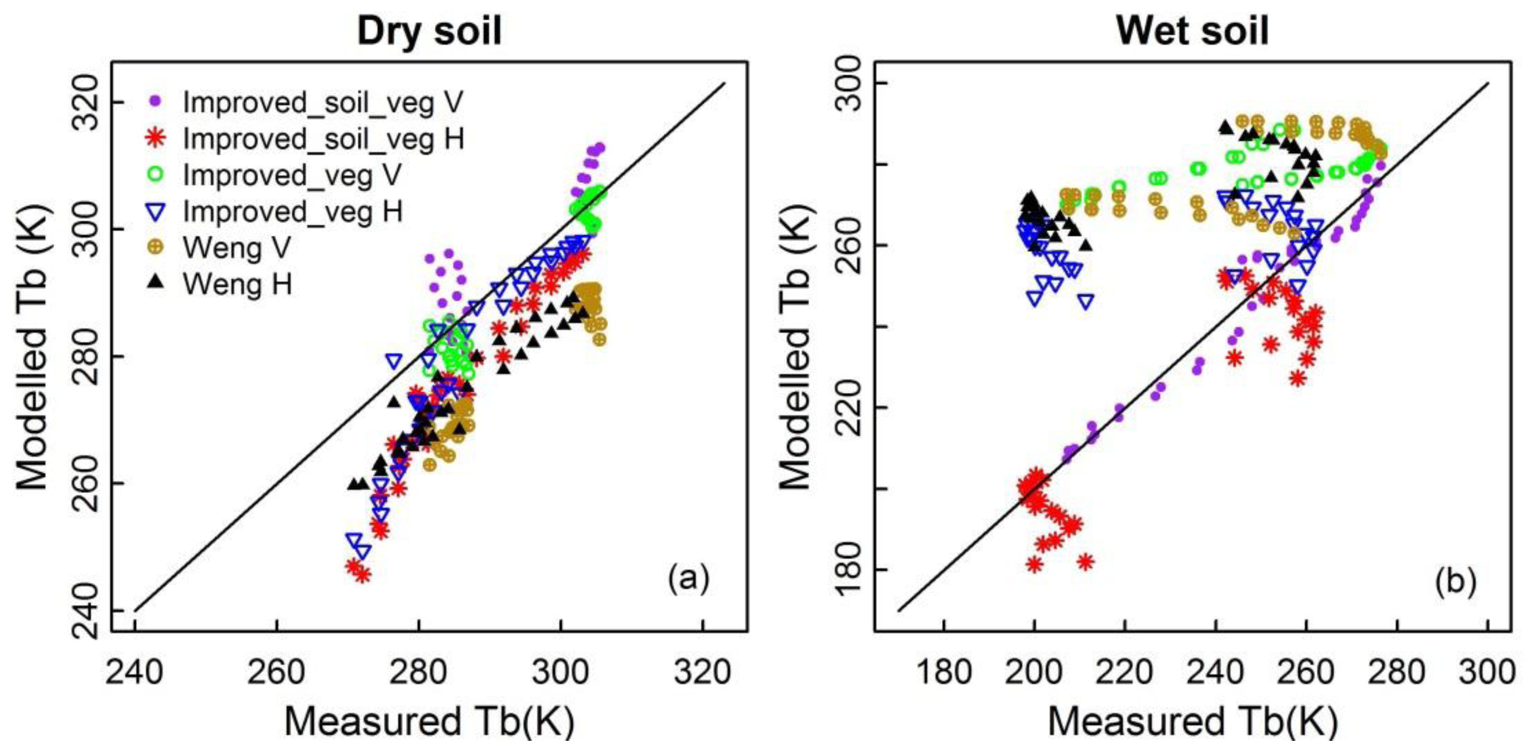
4.3. Discussion
4.3.1. General Discussion of Results

| Models | Weng Model | Improved_veg | Improved_soil_veg | ||||
|---|---|---|---|---|---|---|---|
| Statistics | Dry Soil | Wet Soil | Dry Soil | Wet Soil | Dry Soil | Wet Soil | |
| R2 | V | 0.94 | 0.06 | 0.94 | 0.46 | 0.75 | 0.97 |
| H | 0.92 | 0.08 | 0.90 | 0.08 | 0.93 | 0.83 | |
| RMSE | V | 16.06 | 33.37 | 3.63 | 36.90 | 5.91 | 4.15 |
| H | 12.28 | 43.99 | 9.85 | 41.66 | 12.32 | 14.44 | |
4.3.2. Sources of Uncertainty
5. Conclusions
Acknowledgments
Author Contributions
Conflicts of Interest
References
- Weng, F.Z.; Yan, B.H.; Grody, N.C. A microwave land emissivity model. J. Geophys. Res. 2001, 106, 20115–20123. [Google Scholar] [CrossRef]
- Paloscia, S. Microwave emission from vegetation. In Passive Microwave Remote Sensing of Land-Atmosphere Interactions; Choudhury, B.J., Kerr, Y.H., Njoku, E.G., Pampaloni, P., Eds.; VSP Press: Utrecht, The Netherlands, 1995; pp. 357–374. [Google Scholar]
- Weng, F.Z.; Grody, N.C. Physical retrieval of land surface temperature using the special sensor microwave imager. J. Geophys. Res. 1998, 103, 8839–8848. [Google Scholar] [CrossRef]
- Ferrazzoli, P.; Guerriero, L. Modeling microwave emission from vegetation-covered surfaces: A parametric analysis. In Passive Microwave Remote Sensing of Land-Atmosphere Interactions; Choudhury, B.J., Kerr, Y.H., Njoku, E.G., Pampaloni, P., Eds.; VSP Press: Utrecht, The Netherlands, 1995; pp. 389–402. [Google Scholar]
- Ulaby, F.T.; El-Rayes, M.A. Microwave dielectric spectrum of vegetation. Part II: Dual-dispersion model. IEEE Trans. Geos. Remot. Sens. 1987, GE-25, 550–556. [Google Scholar] [CrossRef]
- Karam, M.A.; Fung, A.K.; Lang, R.H.; Chuahan, N.S. A microwave scattering model for layered vegetation. IEEE Trans. Geosci. Remote Sens. 1992, 30, 767–784. [Google Scholar] [CrossRef]
- Ulaby, F.T.; Sarabandi; McDonald, K.; Whitt, M.; Dobson, M.C. Michigan canopy scattering model. Int. J. Remote Sens. 1990, 11, 1223–1253. [Google Scholar] [CrossRef]
- Tsang, L.; Kong, J.A.; Shin, R.T. Radiative transfer theory for active remote sensing ellipsoidal scatters. Radio Sci. 1984, 19, 629–642. [Google Scholar] [CrossRef]
- Ulaby, F.T.; Moore, R.K.; Fung, A.K. Passive microwave sensing of land. In Microwave Remote Sensing Active and Passive; Artech House Press: Dedham, MA, USA, 1986; Volume III, pp. 1522–1638. [Google Scholar]
- Pampaloni, P.; Paloscia, S. Microwave emission and plant water content: A comparison between field measurements and theory. IEEE Trans. Geosci. Remote Sens. 1986, GE-24, 900–905. [Google Scholar] [CrossRef]
- Wegmuller, U. Remote Sensing Signature Studies on Agricultural Fields with Ground-based Radiometry and Scatterometry. Ph.D. Thesis, University of Berne, Bern, Switzerland, 1990. [Google Scholar]
- Schwank, M.; Matzler, C.; Guglielmetti, M.; Fluhler, H. L-band radiometer measurements of soil water under growing clover grass. IEEE Trans. Geosci. Remote Sens. 2005, 43, 2225–2237. [Google Scholar] [CrossRef]
- Vereecken, H.; Weihermüller, L.; Jonard, F.; Montzka, C. Characterization of crop canopies and water stress related phenomena using microwave remote sensing methods: A review. Vadose Zone J. 2012, 11. [Google Scholar] [CrossRef]
- Choudhury, B.J.; Schmugge, T.J.; Chang, A.; Newton, R.W. Effect of surface roughness on the microwave emission from soils. J. Geophys. Res. 1979, 84, 5699–5706. [Google Scholar] [CrossRef]
- Au, W.C.; Tsang, L.; Shin, R.T.; Kong, J.A. Collective scattering and absorption in microwave interaction with vegetation canopies. Prog. Electromagn. Res. 1996, 14, 181–231. [Google Scholar]
- Kurum, M.; Lang, R.H.; O’Neill, P.E.; Joseph, A.T.; Jackson, T. A first-order radiative transfer model for microwave radiometry of forest canopies at L-band. IEEE Trans. Geosci. Remote Sens. 2011, 49, 3167–3179. [Google Scholar] [CrossRef]
- Wigneron, J.P.; Kerr, Y.H.; Waldtufe, P.; Saleh, K.; Richaume, P. L-band microwave emission of the biosphere (L-MEB) model: Results from calibration against experimental data sets over crop fields. Remote Sens. Environ. 2007, 107, 639–655. [Google Scholar] [CrossRef]
- Mo, T.; Choudhury, B.J.; Schmugge, T.J.; Wang, J.R.; Jackson, T.J. A model for microwave emission from vegetation-covered fields. J. Geophys. Res. 1982, 87, 11229–11237. [Google Scholar] [CrossRef]
- Fung, A.K.; Eom, H.J. Emission from a rayleigh layer with irregular boundaries. J. Quant. Spectrosc. Radiat. Trans. 1981, 26, 397–409. [Google Scholar] [CrossRef]
- Ferrazzoli, P.; Solimini, D.; Luzi, G.; Paloscia, S. Model analysis of backscatter and emission from vegetated terrains. JEWA 1991, 5, 175–193. [Google Scholar] [CrossRef]
- Shi, J.C.; Jiang, L.M.; Zhang, L.X.; Chen, K.S.; Wigneron, J.P.; Chanzy, A. A parameterized multifrequency-polarization surface emission model. IEEE Trans. Geosci. Remote Sens. 2005, 43, 2831–2841. [Google Scholar]
- Zhao, T.J.; Shi, J.C.; Bindlish, R.; Jackson, T.; Cosh, M.; Jiang, L.M. Parametric Exponentially Correlated Surface Emission Model For L-Band Passive Microwave Soil Moisture Retrieval. Available online: http://0-dx-doi-org.brum.beds.ac.uk/10.1016/j.pce.2015.04.001 (accessed on 15 May 2015).
- Chen, K.S.; Wu, T.D.; Tsang, L.; Li, Q.; Shi, J.C.; Fung, A.K. The emission of rough surfaces calculated by the integral equation method with a comparison to a three-dimensional moment method simulations. IEEE Trans. Geosci. Remote Sens. 2003, 41, 90–101. [Google Scholar] [CrossRef]
- Wegmuller, U.; Matzler, C.; Njoku, E. Canopy opacity models. In Passive Microwave Remote Sensing of Land-Atmosphere Interactions; Choudhury, B.J., Kerr, Y.H., Njoku, E.G., Pampaloni, P., Eds.; VSP Press: Utrecht, The Netherlands, 1995; pp. 380–384. [Google Scholar]
- Schiffer, R.; Thielheim, K.O. Light scattering by dielectric needles and disks. J. Appl. Phys. 1979, 50, 2476–2483. [Google Scholar] [CrossRef]
- Le Vine, D.M.; Meneghini, R.; Lang, R.H.; Seker, S.S. Scattering from arbitrarily oriented dielectric disks in the physical optics regime. J. Opt. Soc. Am. 1983, 73, 1255–1262. [Google Scholar] [CrossRef]
- Karam, M.A.; Fung, A.K.; Antar, Y.M.M. Electromagnetic wave scattering from some vegetation samples. IEEE Trans. Geosci. Remote Sens. 1988, 26, 799–808. [Google Scholar] [CrossRef]
- Karam, M.A.; Fung, A.K. Electromagnetic scattering from a layer of finite length, randomly oriented, dielectric, circular cylinders over a rough interface with application to vegetation. Int. J. Remote Sens. 1988, 9, 1109–1134. [Google Scholar] [CrossRef]
- Shi, J.C.; Jackson, T.; Tao, J.; Du, J.; Bindlish, R.; Lu, L.; Chen, K.S. Microwave vegetation indices for short vegetation covers from satellite passive microwave sensor AMSR-E. Remote Sens. Environ. 2008, 112, 4285–4300. [Google Scholar] [CrossRef]
- Zhao, T.J.; Zhang, L.X.; Shi, J.C.; Jiang, L.M. A physically based statistical methodology for surface soil moisture retrieval in the Tibet plateau using microwave vegetation indices. J. Geophys. Res. 2011, 116, D08116. [Google Scholar] [CrossRef]
- Li, X.; Zhang, L.; Weihermuller, L.; Jiang, L.M.; Vereecken, H. Measurement and simulation of topographic effects on passive microwave remote sensing over mountain areas: A case study from the Tibetan Plateau. IEEE Trans. Geosci. Remote Sens. 2014, 52, 1489–1501. [Google Scholar] [CrossRef]
- Zhao, T.; Zhang, L.; Jiang, L.; Chai, L.; Jin, R. A new soil freeze/thaw discriminant algorithm using AMSR-E passive microwave imagery. Hydrol. Process. 2011, 25, 1704–1716. [Google Scholar] [CrossRef]
- Chai, L.N. Vegetation Biomass Inversion Algorithm Study Based on Passive Microwave Remote Sensing. Ph.D. Thesis, Beijing Normal University, Beijing, China, 2010. [Google Scholar]
- Fung, A.K. Introduction: brightness temperature. In Microwave Scattering and Emission Models and Their Applications; Artech House: Dedham, MA, USA, 1994; pp. 16–18. [Google Scholar]
- Ulaby, F.T.; Moore, R.K.; Fung, A.K. Microwave Remote Sensing—Active and Passive Volume I: Microwave Remote Sensing Fundamentals and Radiometry; Artech House: Dedham, MA, USA, 1981; p. 57. [Google Scholar]
- Ferrazzoli, P.; Guerriero, L.; Paloscia, S.; Pampaloni, P.; Solimini, D. Modeling polarization properties of emission from soil covered with vegetation. IEEE Trans. Geosci. Remote Sens. 1992, 30, 157–165. [Google Scholar] [CrossRef]
- Ewe, H.T.; Chuah, H.T. Electromagnetic scattering from an electrically dense vegetation medium. IEEE Trans. Geosci. Remote Sens. 2000, 38, 2093–2105. [Google Scholar] [CrossRef]
© 2015 by the authors; licensee MDPI, Basel, Switzerland. This article is an open access article distributed under the terms and conditions of the Creative Commons Attribution license (http://creativecommons.org/licenses/by/4.0/).
Share and Cite
Xie, Y.; Shi, J.; Lei, Y.; Li, Y. Modeling Microwave Emission from Short Vegetation-Covered Surfaces. Remote Sens. 2015, 7, 14099-14118. https://0-doi-org.brum.beds.ac.uk/10.3390/rs71014099
Xie Y, Shi J, Lei Y, Li Y. Modeling Microwave Emission from Short Vegetation-Covered Surfaces. Remote Sensing. 2015; 7(10):14099-14118. https://0-doi-org.brum.beds.ac.uk/10.3390/rs71014099
Chicago/Turabian StyleXie, Yanhui, Jiancheng Shi, Yonghui Lei, and Yunqing Li. 2015. "Modeling Microwave Emission from Short Vegetation-Covered Surfaces" Remote Sensing 7, no. 10: 14099-14118. https://0-doi-org.brum.beds.ac.uk/10.3390/rs71014099