
Quantitative Estimation of Fluorescence Parameters for Crop Leaves with Bayesian Inversion

 , ,
, ,
Abstract
:
1. Introduction

| Parameter | Definition | Unit | Description |
|---|---|---|---|
| N | Leaf structure parameter | - | Number of compact layers specifying the average number of air/cell wall interfaces within the mesophyll. |
| Cab | Chlorophyll a+b content | μg·cm−2 | Mass of chlorophyll a+b per leaf area. |
| Car | Total carotenoid content | μg·cm−2 | Mass of total carotenoid per leaf area. |
| Cw | Water content | g·cm−2 | Mass of water per leaf area. |
| Cm | Dry matter content | g·cm−2 | Mass of dry matter per leaf area. |
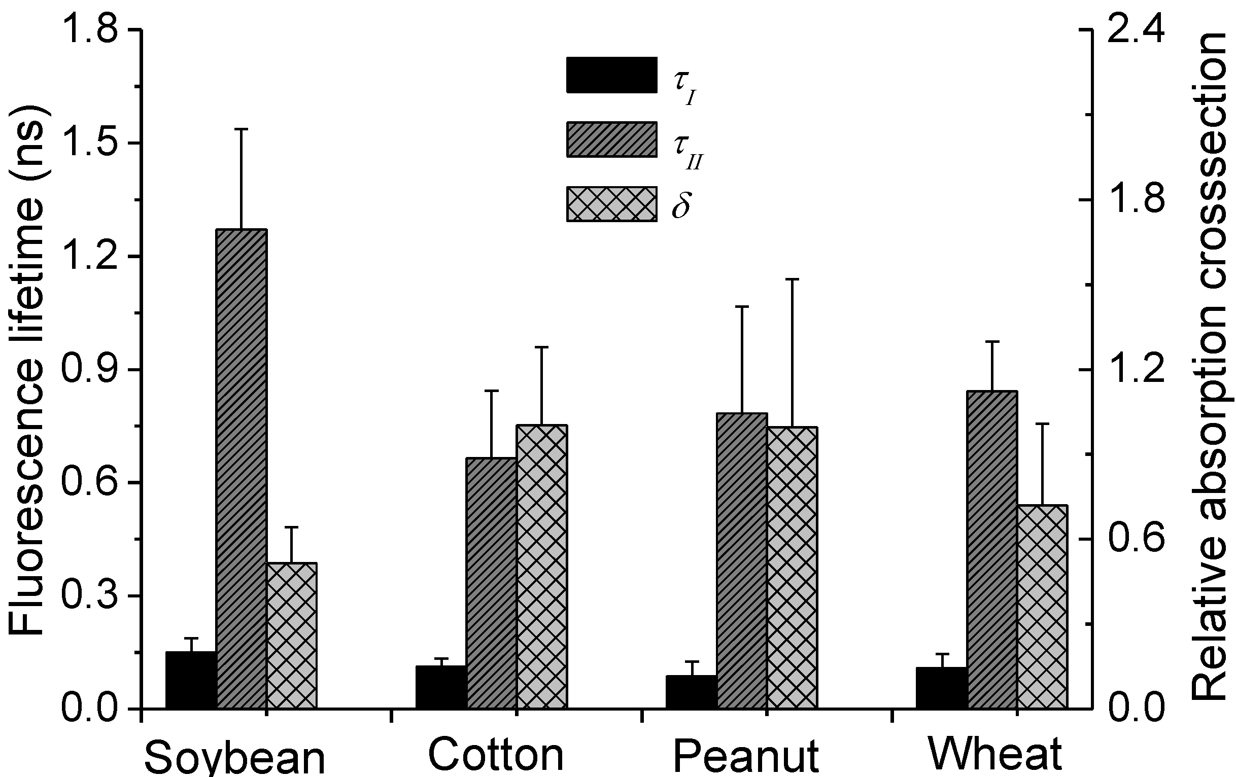
| δ | Relative absorption cross section ratio | - | The relative distribution of light between the two photosystems, which can be approximated by the product of the PSII/PSI antenna size ratio. |
| τI | Fluorescence lifetimes of photosystem I (PSI) | ns | Average time the chlorophyll molecule stays in its excited state before emitting a photon from isolated PSI complexes. |
| τII | Fluorescence lifetimes of photosystem II (PSII) | ns | Average time the chlorophyll molecule stays in its excited state before emitting a photon from isolated PSII complexes. |
2. Materials and Methods
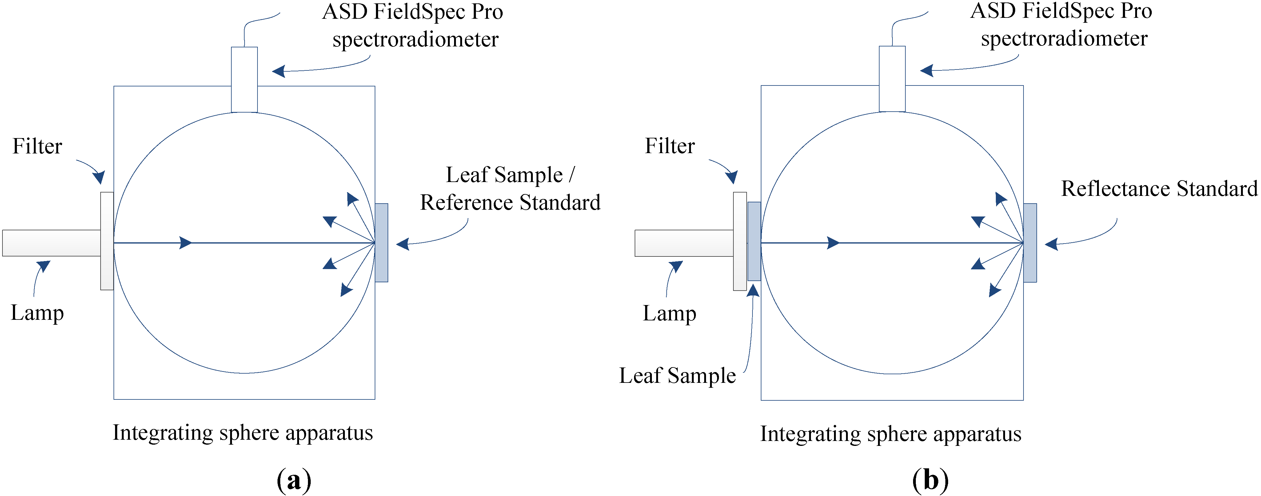
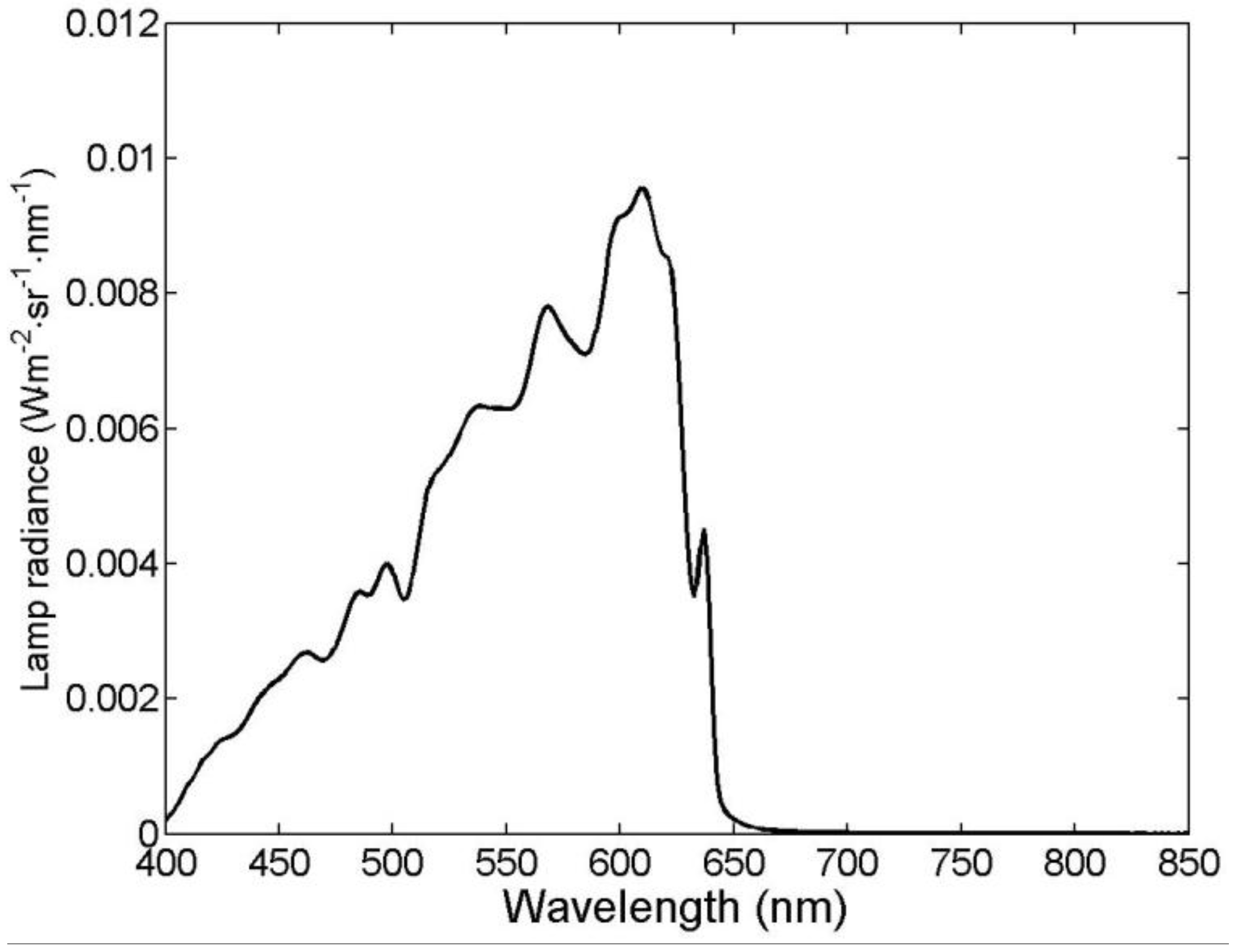
2.1. Experimental Datasets


2.2. Sensitivity Analysis
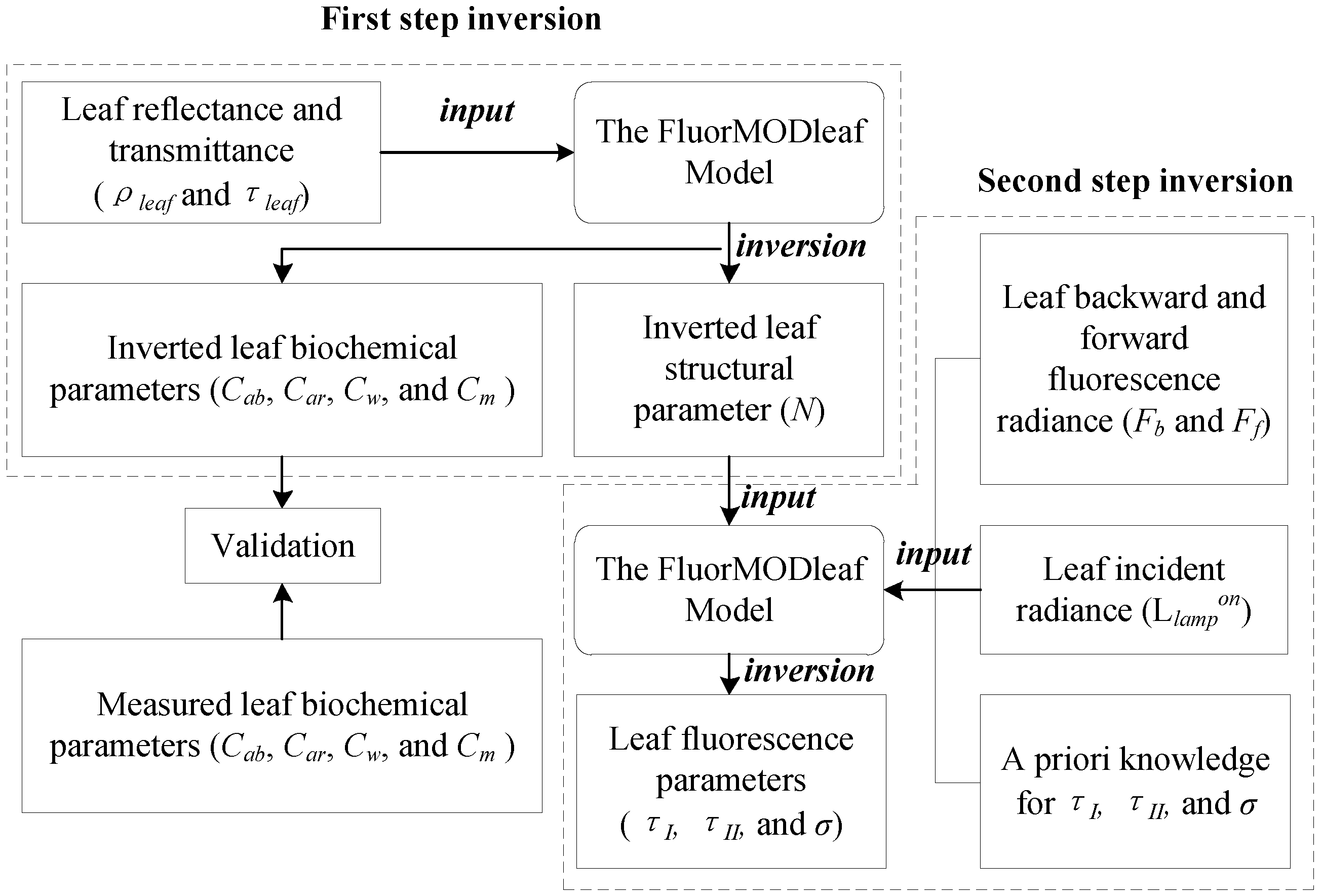
2.3. Inversion Procedure
| Parameter | τI | τII | δ |
|---|---|---|---|
| A priori guess | 0.035 | 0.5 | 1 |
| Variances of the a priori guess | 0.0833 | 0.3333 | 0.48 |

3. Results and Discussion
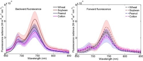
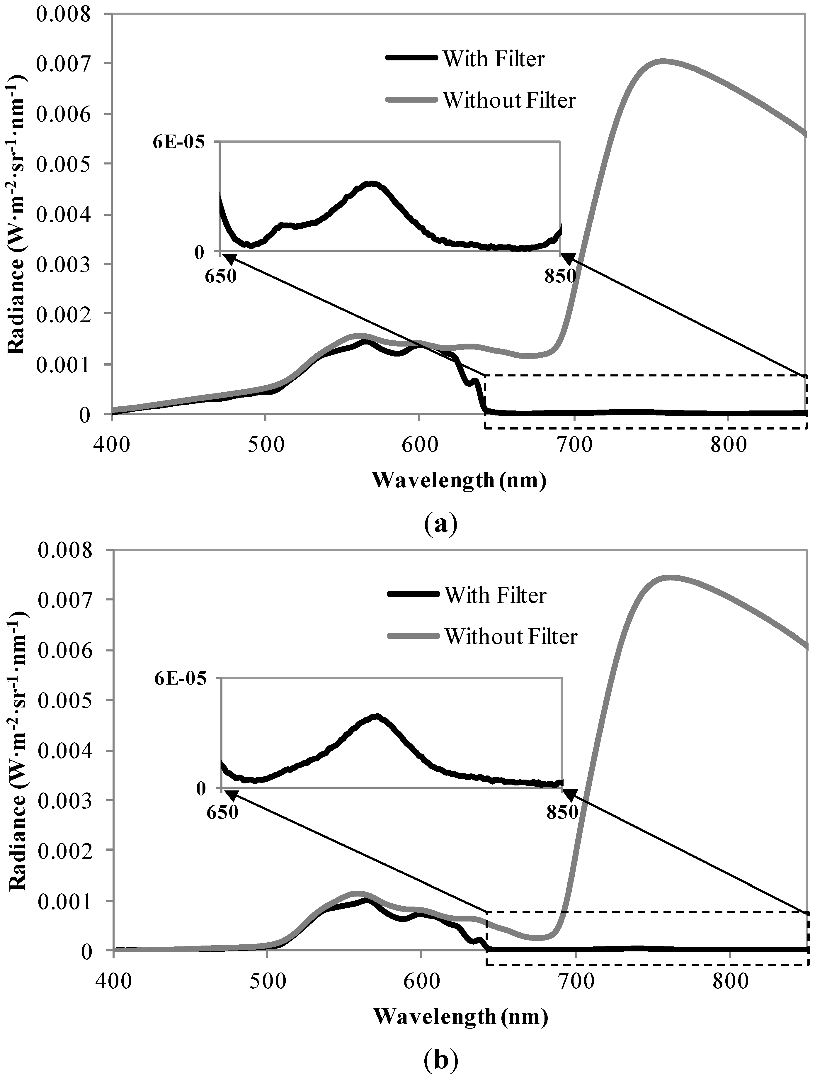
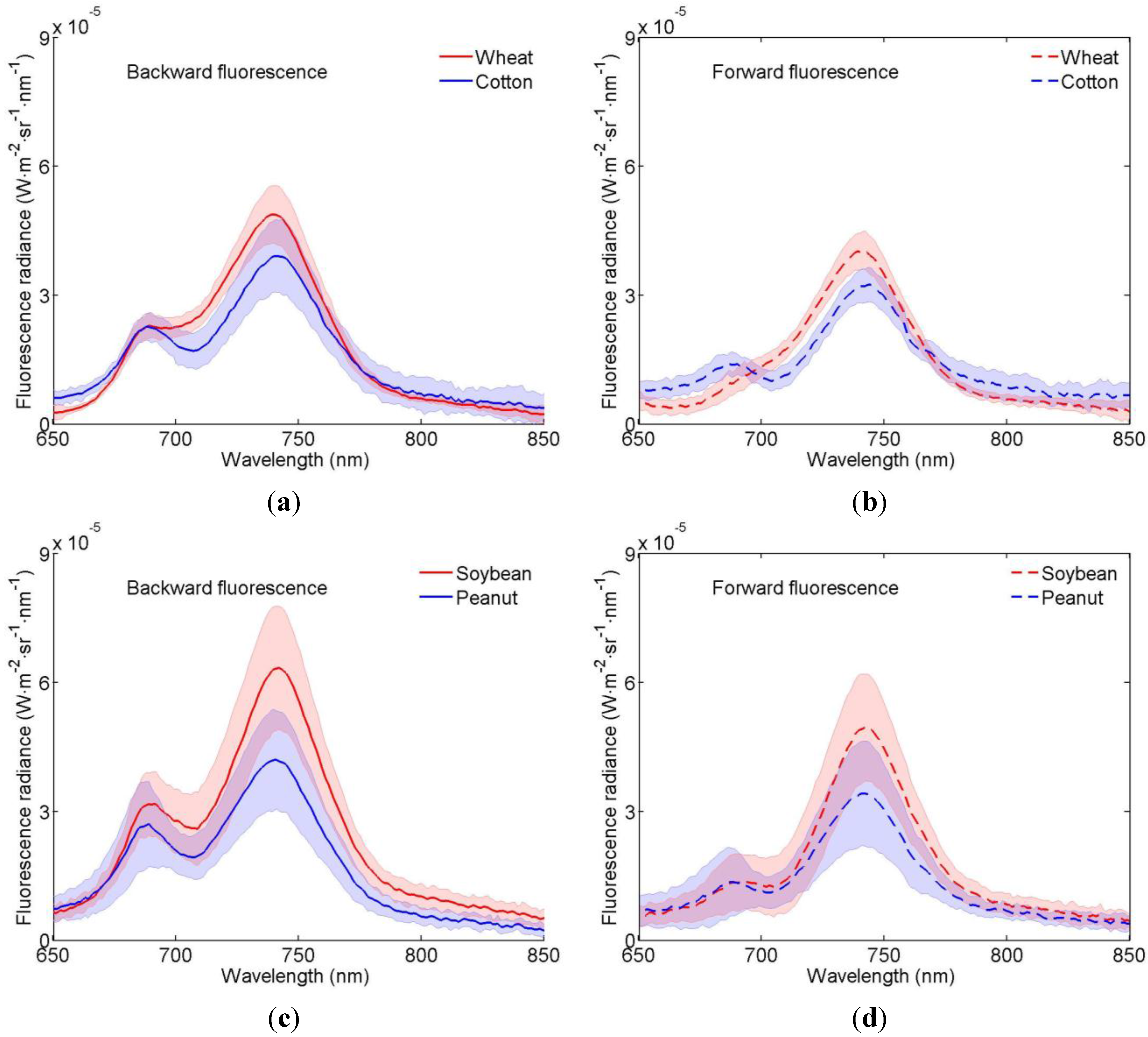
3.1. Distributions of the Fluorescence Spectra


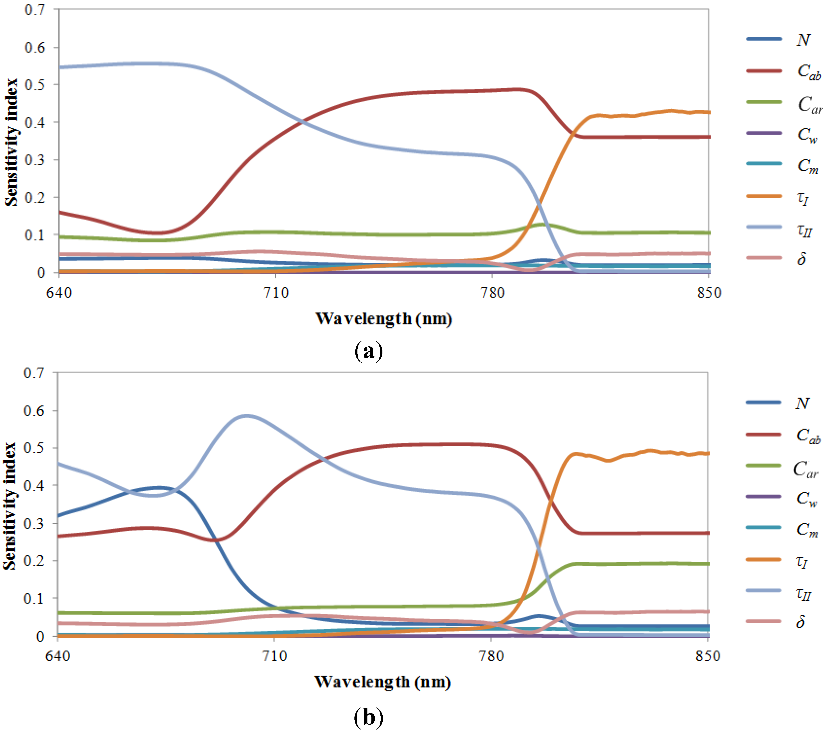
3.2. Results of Sensitivity Analysis for the FluorMODleaf Model

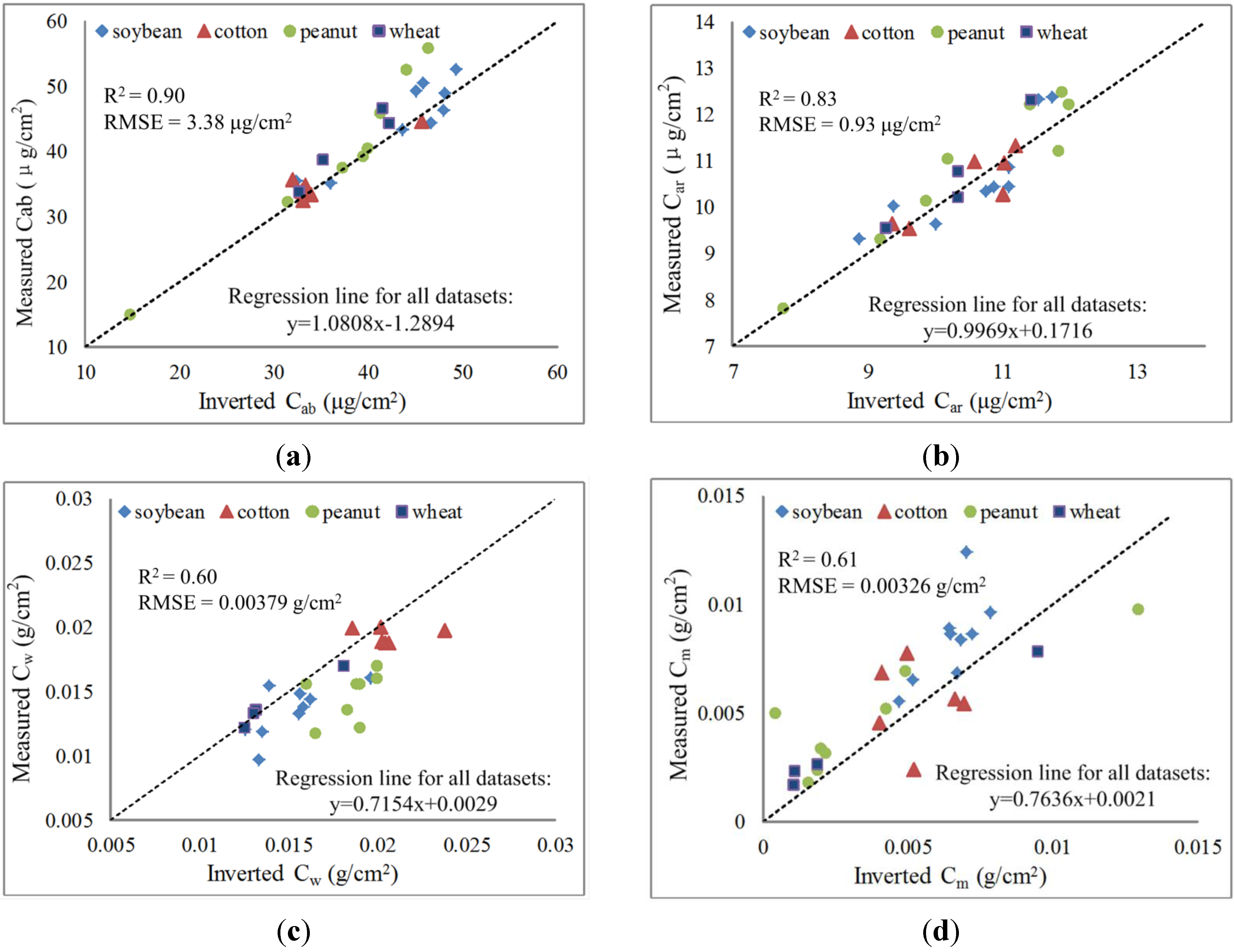
3.3. Retrieval Results of the Leaf Biochemical Contents

3.4. Inversion Results of the Fluorescence Parameters


3.5. Potential and Limitations of Applying Model Inversion for the Retrieval of Leaf Fluorescence Parameters
4. Conclusions
Acknowledgments
Author Contributions
Conflicts of Interest
References
- Meroni, M.; Rossini, M.; Guanter, L.; Alonso, L.; Rascher, U.; Colombo, U.; Moreno, J. Remote sensing of solar-induced chlorophyll fluorescence: Review of methods and applications. Remote Sens. Environ. 2009, 113, 2037–2051. [Google Scholar] [CrossRef]
- Huang, Y.; Thomson, S.J.; Molin, W.T.; Reddy, K.N.; Yao, H. Early detection of soybean plant injury from glyphosate by measuring chlorophyll reflectance and fluorescence. J. Agric. Sci. 2012, 4, 117–124. [Google Scholar] [CrossRef]
- Zhao, F.; Guo, Y.; Huang, Y.; Reddy, K.N.; Zhao, Y.; Molin, W.T. Detection of the onset of glyphosate-induced soybean plant injury through chlorophyll fluorescence signal extraction and measurement. J. Appl. Remote Sens. 2015, 9. [Google Scholar] [CrossRef]
- Guanter, L.; Zhang, Y.; Jung, M.; Joiner, J.; Voigta, M.; Berry, J.A.; Frankenberg, C.; Huete, A.R.; Zarco-Tejada, P.; Lee, J.-E.; et al. Global and time-resolved monitoring of crop photosynthesis with chlorophyll fluorescence. Proc. Natl. Acad. Sci. USA 2014, 111, E1327–E1333. [Google Scholar] [CrossRef] [PubMed]
- Sušila, P.; Nauš, J. A Monte Carlo study of the chlorophyll fluorescence emission and its effect on the leaf spectral reflectance and transmittance under various conditions. Photochem. Photobiol. Sci. 2007, 6, 894–902. [Google Scholar] [CrossRef] [PubMed]
- Pedrós, R.; Goulas, Y.; Jacquemoud, S.; Louis, J.; Moya, I. FluorMODleaf: A new leaf fluorescence emission model based on the PROSPECT model. Remote Sens. Environ. 2010, 114, 155–167. [Google Scholar] [CrossRef]
- Verhoef, W. Modeling vegetation fluorescence observations. In Proceedings of the EARSel 7th SIG-Imaging Spectroscopy Workshop, Edinburgh, UK, 11–13 April 2011.
- Miller, J.R.; Berger, M.; Goulas, Y.; Jacquemoud, S.; Louis, J.; Mohammed, G.; Moise, N.; Moreno, J.; Moya, I.; Pedrós, R.; et al. Development of A Vegetation Fluorescence Canopy Model; ESTEC Contract No. 1635/02/NL/FF; ESA Scientific and Technical Publications Branch, ESTEC: Paris, French, 2015. [Google Scholar]
- Feret, J.-B.; François, C.; Asner, G.P.; Gitelson, A.A.; Martin, R.E.; Bidel, L.P.R.; Ustin, S.L.; Le Maire, G.; Jacquemoud, S. PROSPECT-4 and 5: Advances in the leaf optical properties model separating photosynthetic pigments. Remote Sens. Environ. 2008, 112, 3030–3043. [Google Scholar] [CrossRef]
- Jacquemoud, S.; Baret, F. PROSPECT: A model of leaf optical properties spectra. Remote Sens. Environ. 1990, 34, 75–91. [Google Scholar] [CrossRef]
- Li, X.; Gao, F.; Wang, J.; Strahler, A. A priori knowledge accumulation and its application to linear BRDF model inversion. J. Geophys. Res. D: Atmos. 2001, 106, 11925–11935. [Google Scholar] [CrossRef]
- Laurent, V.C.E.; Schaepman, M.E.; Verhoef, W.; Weyermann, J.; Chávez, R.O. Bayesian object-based estimation of LAI and chlorophyll from a simulated Sentinel-2 top-of-atmosphere radiance image. Remote Sens. Environ. 2014, 140, 318–329. [Google Scholar] [CrossRef]
- Wang, Y.; Li, X.; Nashed, Z.; Zhao, F.; Yang, H.; Guan, Y.; Zhang, H. Regularized kernel-based BRDF model inversion method for ill-posed land surface parameter retrieval. Remote Sens. Environ. 2007, 111, 36–50. [Google Scholar] [CrossRef]
- Laurent, V.C.E.; Verhoef, W.; Damm, A.; Schaepman, M.E.; Clevers, J.G.P.W. A Bayesian object-based approach for estimating vegetation biophysical and biochemical variables from at-sensor APEX data. Remote Sens. Environ. 2013, 139, 6–17. [Google Scholar] [CrossRef]
- Zarco-Tejada, P.J.; Miller, J.R.; Mohammed, G.H.; Noland, T.L. Chlorophyll fluorescence effects on vegetation apparent reflectance: I. Leaf-Level measurements and model simulation. Remote Sens. Environ. 2000, 74, 582–595. [Google Scholar] [CrossRef]
- Zhang, Y. Studies on Passive Sensing of Plant Chlorophyll Florescence and Application of Stress Detection. Ph.D. Thesis, Zhejiang University, Hangzhou, China, May 2006; pp. 24–27. [Google Scholar]
- LI-COR Inc. LI-COR LI-1800-12 Integrating Sphere Instruction Manual; LI-COR Inc.: Lincoln, NE, USA, 1983. [Google Scholar]
- Lichtenthaler, H.K.; Buschmann, C. Extraction of photosynthetic tissues: Chlorophylls and carotenoids. In Current Protocols in Food Analytical Chemistry; Wrolstad, R.E., Acree, T.E., Decker, E.A., Penner, M.H., Reid, D.S., Schwarts, S.J., Eds.; John Wiley and Sons: New York, NY, USA, 2001; p. F4.2.1-6. [Google Scholar]
- Saltelli, A.; Ratto, M.; Andres, T.; Campolongo, F.; Cariboni, J.; Gatelli, D.; Saisana, M.; Tarantola, S. Global Sensitivity Analysis, the Primer; John Wiley & Sons Ltd.: West Sussex, UK, 2008. [Google Scholar]
- Saltelli, A.; Tarantola, S.; Chan, K. A quantitative, model independent method for global sensitivity analysis of model output. Technometrics 1999, 41, 39–56. [Google Scholar] [CrossRef]
- Zhao, F.; Guo, Y.; Huang, Y.; Reddy, K.N.; Lee, M.A.; Fletcher, R.S.; Thomson, S.J. Early detection of crop injury from herbicide glyphosate by leaf biochemical parameter inversion. Int. J. Appl. Earth Observ. Geoinf. 2014, 31, 78–85. [Google Scholar] [CrossRef]
- Zhao, F.; Huang, Y.; Guo, Y.; Reddy, K.N.; Lee, M.A.; Fletcher, R.S.; Thomson, S.J.; Zhao, H. Early detection of crop injury from glyphosate on soybean and cotton using plant leaf hyperspectral data. Remote Sens. 2014, 6, 1538–1563. [Google Scholar] [CrossRef]
- Liu, Q. Study on Component Temperature Inversion Algorithm and the Scale Structure for Remote Sensing Pixel. Ph.D. Thesis, Institute of Remote Sensing Applications, Chinese Academy of Sciences, Beijing, China, May 2002. [Google Scholar]
- Van Wittenberghe, S.; Alonso, L.; Verrelst, J.; Moreno, J.; Samson, R. Bidirectional sun-induced chlorophyll fluorescence emission is influenced by leaf structure and light scattering properties—A bottom-up approach. Remote Sens. Environ. 2015, 158, 169–179. [Google Scholar] [CrossRef]
- Van Wittenberghe, S.; Alonso, L.; Verrelst, J.; Verrelst, I.; Delegido, J.; Veroustraete, F.; Veroustraete, R.; Moreno, J.; Samson, R. Upward and downward solar-induced chlorophyll fluorescence yield indices of four tree species as indicators of traffic pollution in Valencia. Environ. Poll. 2013, 173, 29–37. [Google Scholar] [CrossRef] [PubMed]
- Van Wittenberghe, S.; Alonso, L.; Verrelst, J.; Hermans, I.; Valcke, R.; Veroustraete, F.; Moreno, J.; Samson, R. A field study on solar-induced chlorophyll fluorescence and pigment parameters along a vertical canopy gradient of four tree species in an urban environment. Sci. Total Environ. 2014, 466–467, 185–194. [Google Scholar] [CrossRef] [PubMed]
- Louis, J.; Cerovic, Z.G.; Moya, I. Quantitative study of fluorescence excitation and emission spectra of bean leaves. J. Photochem. Photobiol. B 2006, 85, 65–71. [Google Scholar] [CrossRef] [PubMed]
- Zarco-Tejada, P.J.; Berni, J.A.J.; Suárez, L.; Sepulcre-Cantó, G.; Morales, F.; Miller, J.R. Imaging chlorophyll fluorescence with an airborne narrow-band multispectral camera for vegetation stress detection. Remote Sens. Environ. 2009, 113, 1262–1275. [Google Scholar] [CrossRef]
- Zarco-Tejada, P.J.; González-Dugo, V.; Berni, J.A.J. Fluorescence, temperature and narrow-band indices acquired from a UAV platform for water stress detection using a micro-hyperspectral imager and a thermal camera. Remote Sens. Environ. 2012, 117, 322–337. [Google Scholar] [CrossRef]
- Naumann, J.C.; Young, D.R.; Anderson, J.E. Linking leaf chlorophyll fluorescence properties to physiological responses for detection of salt and drought stress in coastal plant species. Physiol. Plant. 2007, 131, 422–433. [Google Scholar] [CrossRef] [PubMed]
- Verhoef, W. Light scattering by leaves with application to canopy reflectance modelling: The SAIL model. Remote Sens. Environ. 1984, 16, 125–178. [Google Scholar] [CrossRef]
- Van der Tol, C.; Verhoef, W.; Timmermans, J.; Verhoef, A.; Su, X. An integrated model of soil-canopy spectral radiances, photosynthesis, fluorescence, temperature and energy balance. Biogeosciences 2009, 6, 3109–3129. [Google Scholar] [CrossRef]
- Zhao, F.; Gu, X.; Verhoef, W.; Wang, Q.; Yu, T.; Liu, Q.; Huang, H.; Qin, W.; Chen, L.; Zhao, H. A spectral directional reflectance model of row crops. Remote Sens. Environ. 2010, 114, 265–285. [Google Scholar] [CrossRef]
- Zhao, F.; Li, Y.; Dai, X.; Verhoef, W.; Guo, Y.; Shang, H.; Gu, X.; Huang, Y.; Yu, T.; Huang, J. Simulated impact of sensor field of view and distance on field measurements of bidirectional reflectance factors for row crops. Remote Sens. Environ. 2015, 156, 129–142. [Google Scholar] [CrossRef]
© 2015 by the authors; licensee MDPI, Basel, Switzerland. This article is an open access article distributed under the terms and conditions of the Creative Commons Attribution license (http://creativecommons.org/licenses/by/4.0/).
Share and Cite
Zhao, F.; Guo, Y.; Huang, Y.; Verhoef, W.; Van der Tol, C.; Dai, B.; Liu, L.; Zhao, H.; Liu, G. Quantitative Estimation of Fluorescence Parameters for Crop Leaves with Bayesian Inversion. Remote Sens. 2015, 7, 14179-14199. https://0-doi-org.brum.beds.ac.uk/10.3390/rs71014179
Zhao F, Guo Y, Huang Y, Verhoef W, Van der Tol C, Dai B, Liu L, Zhao H, Liu G. Quantitative Estimation of Fluorescence Parameters for Crop Leaves with Bayesian Inversion. Remote Sensing. 2015; 7(10):14179-14199. https://0-doi-org.brum.beds.ac.uk/10.3390/rs71014179
Chicago/Turabian StyleZhao, Feng, Yiqing Guo, Yanbo Huang, Wout Verhoef, Christiaan Van der Tol, Bo Dai, Liangyun Liu, Huijie Zhao, and Guang Liu. 2015. "Quantitative Estimation of Fluorescence Parameters for Crop Leaves with Bayesian Inversion" Remote Sensing 7, no. 10: 14179-14199. https://0-doi-org.brum.beds.ac.uk/10.3390/rs71014179