
Increasing the Accuracy of Mapping Urban Forest Carbon Density by Combining Spatial Modeling and Spectral Unmixing Analysis

 , ,
, ,
Abstract
:
1. Introduction
1.1. Forest Carbon Modeling
1.2. Urban Forest Carbon Modeling
1.3. Spectral Mixture Analysis
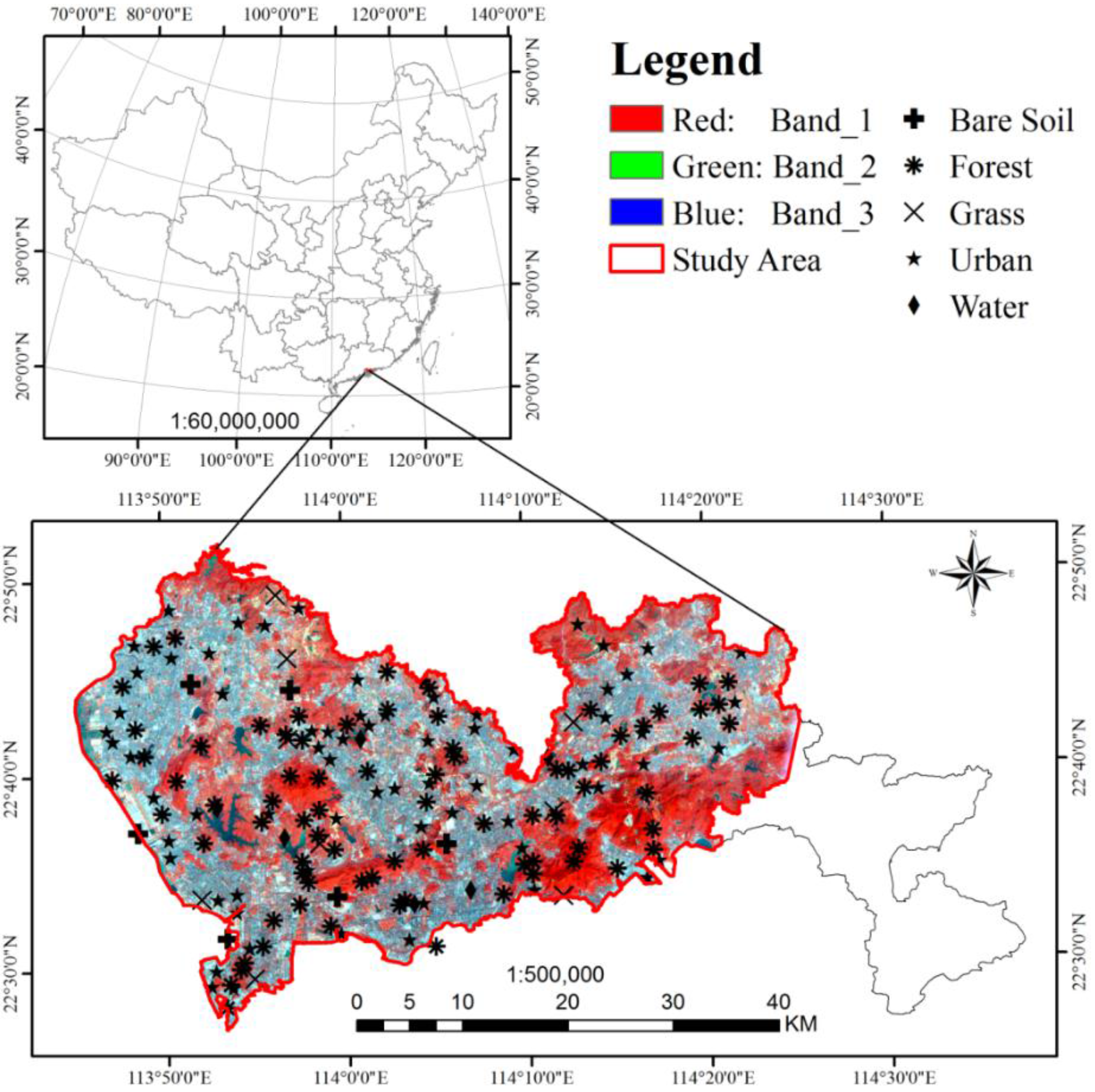
2. Study Area and Datasets

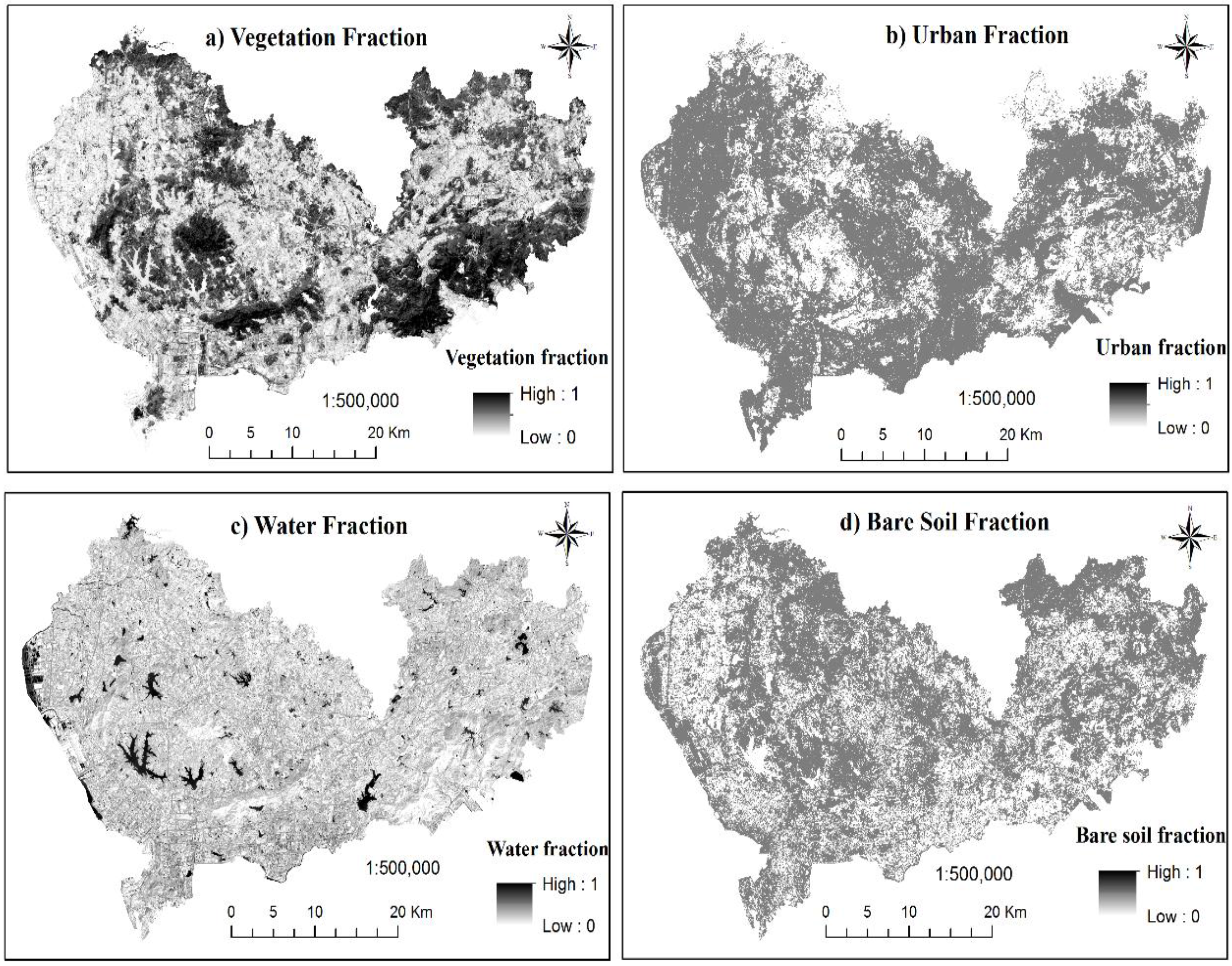
3. Methods

| Spectral Variables | Definitions of Spectral Variables | # of SV |
|---|---|---|
| Original | Landsat 8: band1-coastal aerosol, band2-blue, band3-green (GRN), band4-RED, band5-near infrared (NIR), band6-shortwave infrared 1 (SWIR1), band7-shortwave infrared 2 (SWIR2) and band8-cirrus | 8 |
| Inversions of bands | 8 | |
| Simple two-band ratios | , | 42 |
| Three-band ratios | , | 106 |
| Difference vegetation indices | 42 | |
| Shortwave infrared-visible band ratio | 1 | |
| Normalized difference vegetation index | 1 | |
| Modified normalized difference vegetation index | 1 | |
| Red-green vegetation index | 1 | |
| Reduced simple ratio | 1 | |
| Soil adjusted vegetation index | , l=0.1, 0.25, 0.3, 0.5 | 4 |
| Atmospherically resistant vegetation index | 1 | |
| Enhanced vegetation index | 1 | |
| Principal component analysis | The first 3 PCs from Principal component analysis (PCA) | 3 |
| Texture measures | Grey-level co-occurrence matrix-based texture measures including mean, angular second moment, contrast, correlation, dissimilarity, entropy, homogeneity and variance | 64 |
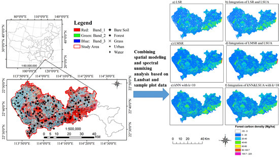
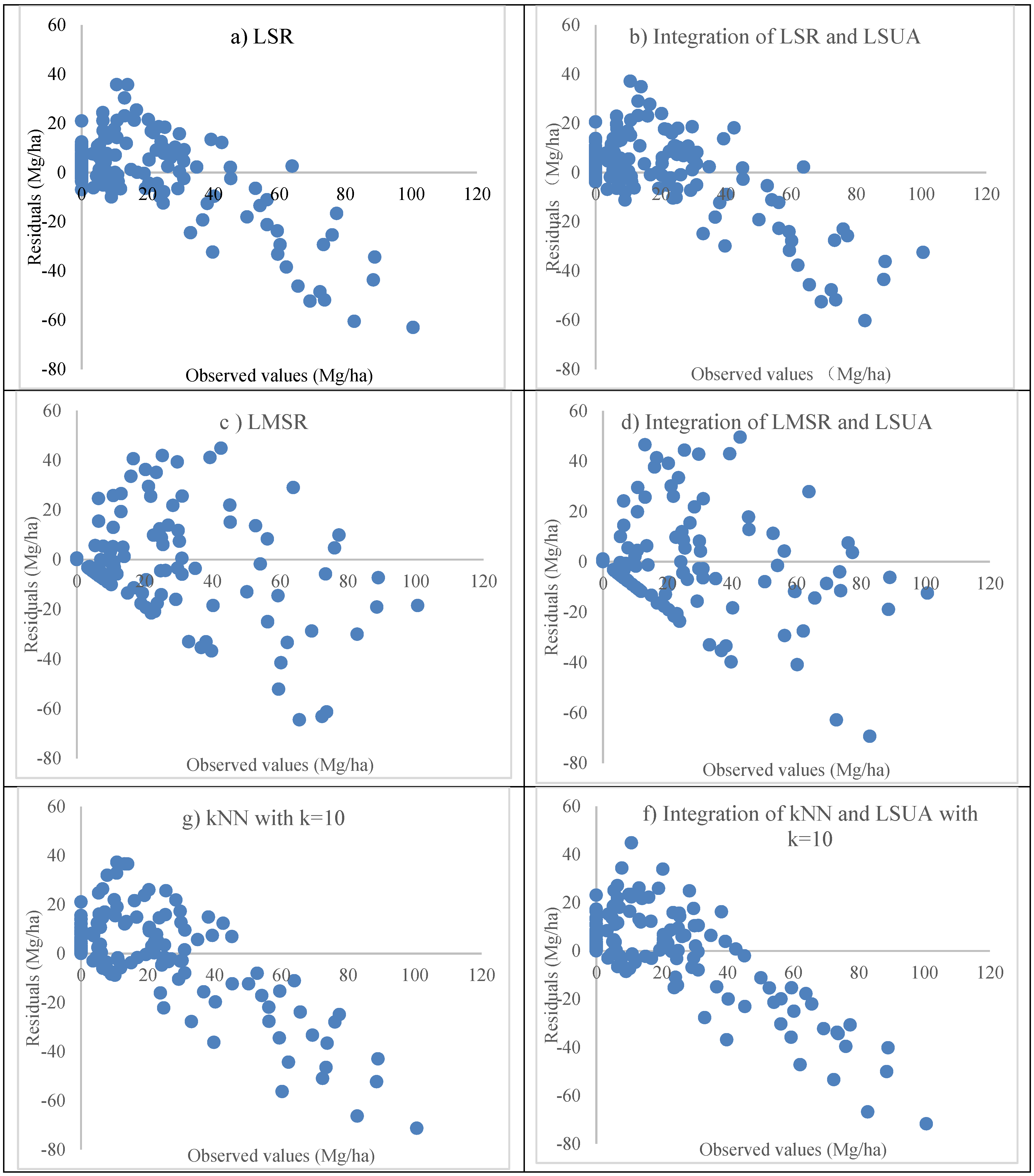
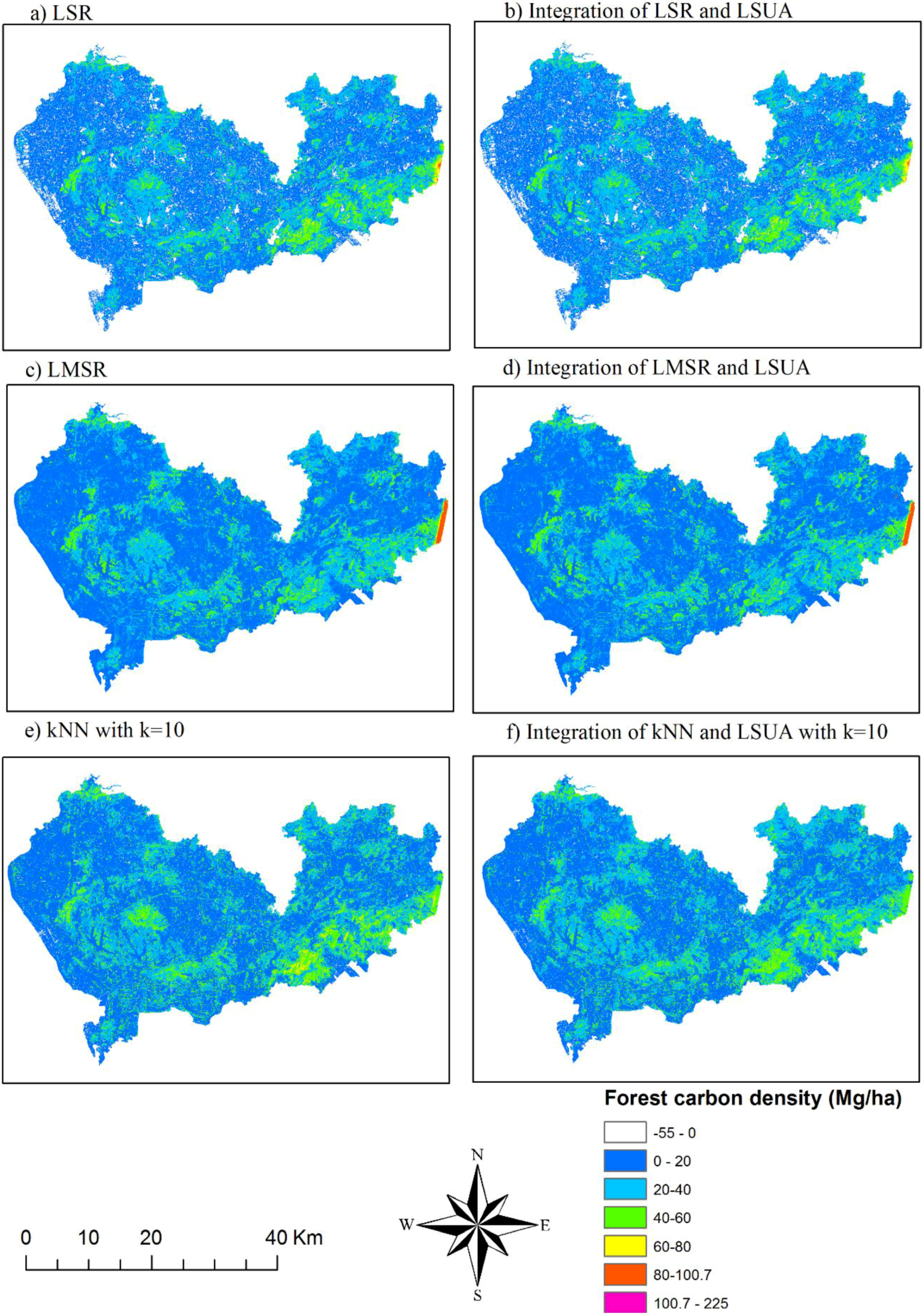
4. Results
| Number of Plots | Minimum (Mg/ha) | Maximum (Mg/ha) | Sample Mean (Mg/ha) | Standard Deviation (Mg/ha) | Coefficient of Variation (%) |
|---|---|---|---|---|---|
| 161 | 0 | 100.65 | 18.54 | 23.33 | 125.88 |

| Method | Mean (Mg/ha) | R2 | RMSE (Mg/ha) | ||
|---|---|---|---|---|---|
| LSR | 18.56 | 0.514 | 16.67 | 17.74 | 1.78 |
| LSR&LSUA | 18.76 | 0.514 | 16.13 | 17.96 | 1.67 |
| LMSR | 17.16 | 0.537 | 17.72 | 15.73 | 2.01 |
| LMSR&LSUA | 17.99 | 0.578 | 17.08 | 16.57 | 1.87 |
| k | Mean (Mg/ha) | R2 | RMSE (Mg/ha) | ||
|---|---|---|---|---|---|
| kNN based on the significant spectral variables from LSR | |||||
| 3 | 18.26 | 0.298 | 20.51 | 19.03 | 2.70 |
| 5 | 18.37 | 0.333 | 19.54 | 18.98 | 2.45 |
| 7 | 18.49 | 0.356 | 19.02 | 18.94 | 2.32 |
| 10 | 18.41 | 0.388 | 18.37 | 18.79 | 2.16 |
| Integration of kNN based on the significant spectral variables from LSR with LSUA | |||||
| 3 | 18.11 | 0.303 | 20.32 | 18.66 | 2.65 |
| 5 | 18.35 | 0.363 | 18.94 | 18.83 | 2.31 |
| 7 | 18.28 | 0.389 | 18.40 | 18.62 | 2.17 |
| 10 | 18.10 | 0.397 | 18.19 | 18.33 | 2.12 |
| kNN based on the significant spectral variables from LMSR | |||||
| 3 | 18.32 | 0.322 | 20.00 | 18.97 | 2.56 |
| 5 | 18.57 | 0.354 | 19.14 | 19.07 | 2.35 |
| 7 | 18.31 | 0.378 | 18.56 | 18.71 | 2.21 |
| 10 | 18.30 | 0.394 | 18.22 | 18.56 | 2.13 |
| Integration of kNN based on the significant spectral variables from LMSR with LSUA | |||||
| 3 | 18.02 | 0.343 | 19.39 | 18.75 | 2.41 |
| 5 | 18.26 | 0.373 | 18.61 | 18.97 | 2.22 |
| 7 | 18.14 | 0.403 | 18.07 | 18.66 | 2.09 |
| 10 | 18.29 | 0.415 | 17.84 | 18.61 | 2.04 |


5. Discussion
6. Conclusions
Acknowledgments
Author Contributions
Conflicts of Interest
References
- Churkina, G.; Brown, D.; Keoleian, G. Carbon stored in human settlements: The conterminous United States. Glob. Change Biol. 2010, 16, 135–143. [Google Scholar] [CrossRef]
- Strohbach, M.W.; Arnold, E.; Haase, D. The carbon footprint of urban green space-A life cycle approach. Landsc. Urban Plan. 2012, 104, 220–229. [Google Scholar] [CrossRef]
- Fang, J.; Chen, A.; Peng, C.; Zhao, S.; Ci, L. Changes in forest biomass carbon storage in China between 1949 and 1998. Science 2002, 292, 2320–2322. [Google Scholar] [CrossRef] [PubMed]
- Grace, J.; Lloyd, J.; Mcintyre, J.; Miranda, A.C. Carbon dioxide uptake by an undisturbed tropical rain forest in Southwest Amazonia, 1992 to 1993. Science 1995, 270, 778. [Google Scholar] [CrossRef]
- Schimel, D.S.; House, J.I.; Hibbard, K.A.; Bousquet, P.; Ciais, P.; Peylin, P.; Braswell, B.H.; Apps, M.J.; Baker, D.; Bondeau, A.; et al. Recent patterns and mechanism of carbon exchange by terrestrial ecosystems. Nature 2001, 414, 169–172. [Google Scholar] [CrossRef] [PubMed]
- Smith, J.E.; Heath, L.S. Carbon stocks and stock changes in U.S. forests and Appendix C. In U.S. Agriculture and Forestry Greenhouse Gas Inventory: 1990–2005; Technical Bulletin No. 1921; Global Change Program Office, Office of the Chief Economist: Washington, DC, USA, 2008. Available online: http://www.usda.gov/oce/global_change/AFGGInventory1990_2005.htm/ (accessed on 28 August 2015). [Google Scholar]
- US Climate Change Science Program. The North American Carbon Budget and Implications for the Global Carbon Cycle. Available online: http://www.cfr.org/climate-change/north-american-carbon-budget-implications-global-carbon-cycle/p14868/ (accessed on 28 August 2015).
- Lu, D.; Chen, Q.; Wang, G.; Liu, L.; Moran, E. A survey of remote sensing-based aboveground biomass estimation methods. Int. J. Digit. Earth 2014. [Google Scholar] [CrossRef]
- Wang, G.; Oyana, T.; Zhang, M.; Adu-Prah, S.; Zeng, S.; Lin, H.; Se, J. Mapping and spatial uncertainty analysis of forest vegetation carbon by combining national forest inventory data and satellite images. For. Ecol. Manage. 2009, 258, 1275–1283. [Google Scholar] [CrossRef]
- Lu, D. The potential and challenge of remote sensing-based biomass estimation. Int. J. Remote Sens. 2006, 27, 1297–1328. [Google Scholar] [CrossRef]
- Intergovermental Panel on Climate Change (IPCC). Land Use, Land-Use Change and Forestry; Cambridge University Press: Cambridge, UK, 2000. [Google Scholar]
- Yang, H.; Zhou, Q.; Chen, Z.; Zhang, S. Estimation methods and application analysis of forest carbon stock. J. Geoinf. Sci. 2007, 9, 5–12. (In Chinese) [Google Scholar]
- Zhou, X.; Wang, Z.; Zhu, Q. A Review of global climate change and forest carbon sequestration. Shanxi For. Sci. Tech. 2011, 2, 47–52. [Google Scholar]
- Fu, D.; Chen, B.; Zhang, H.; Wang, J.; Black, A.; Amiro, B.D. Estimating landscape net ecosystem exchange at high spatial-temporal resolution based on Landsat data, an improved upscaling model framework, and eddy covariance flux measurements. Remote Sens. Environ. 2014, 141, 90–104. [Google Scholar] [CrossRef]
- Landsberg, J.J.; Waring, R.H. A generalized model of forest productivity using simplified concepts of radiation-use efficiency, carbon balance, and partitioning. For. Ecol. Manage. 1997, 95, 209–228. [Google Scholar] [CrossRef]
- Running, S.W.; Coughlan, J.C. A general model of forest ecosystem processes for regional applications I. Hydrologic balance, canopy gas exchange and primary production processes. Ecol. Model. 1988, 42, 125–154. [Google Scholar] [CrossRef]
- Kimball, J.S.; Keyser, A.R.; Running, S.W.; Saatch, S.S. Regional assessment of boreal forest productivity using an ecological process model and remote sensing parameter maps. Tree Physiol. 2000, 20, 761–775. [Google Scholar] [CrossRef] [PubMed]
- Running, S.W.; Hunt, E.R., Jr. Generalization of a forest ecosystem process model for other biomes, BIOME-BGC, and an application for global scale models. In Scaling Physiological Processes: Leaf to Globe; Ehleringer, J.R., Field, C.B., Eds.; Academic Press, Inc.: San Diego, CA, USA, 1993; pp. 141–158. [Google Scholar]
- Neumann, M.; Zhao, M.; Kindermann, G.; Hasenauer, H. Comparing MODIS net primary production estimates with terrestrial national forest inventory data in Austria. Remote Sens. 2015, 7, 3878–3906. [Google Scholar] [CrossRef]
- Lu, D.; Chen, Q.; Wang, G.; Moran, E.; Batistella, M.; Zhang, M.; Laurin, G.V.; Saah, D. Estimation and uncertainty analysis of aboveground forest biomass with Landsat and LiDAR data: Brief overview and case studies. Int. J. For. Res. 2012, 1, 1–16. [Google Scholar]
- Tian, X.; Su, Z.; Chen, E.; Li, Z.; van der Tol, C.; Guo, J.; He, Q. Estimation of forest above-ground biomass using multi-parameter remote sensing data over a cold and arid area. Int. J. Appl. Earth Observ. Geoinf. 2012, 14, 160–168. [Google Scholar] [CrossRef]
- Wang, G.; Zhang, M.; Gertner, G.Z.; Oyana, T.; McRoberts, R.E.; Ge, H. Uncertainties of mapping forest carbon due to plot locations using national forest inventory plot and remotely sensed data. Scand. J. For. Res. 2011, 26, 360–373. [Google Scholar] [CrossRef]
- Wang, G.; Zhang, M. Upscaling with conditional co-simulation for mapping aboveground forest carbon. In Scale Issue in Remote Sensing; Weng, Q., Ed.; John Wiley and Sons: Hobboken, NJ, USA, 2014; pp. 108–125. [Google Scholar]
- Zhang, M.; Lin, H.; Zeng, S.; Li, J.; Shi, J.; Wang, G. Impacts of plot location errors on accuracy of mapping and up-scaling aboveground forest carbon using sample plot and Landsat TM data. IEEE Geosci. Remote Sens. Lett. 2013, 10, 1483–1487. [Google Scholar] [CrossRef]
- Foody, G.M.; Cutler, M.E.; McMorrow, J.; Pelz, D.; Tangki, H.; Boyd, D.S.; Douglas, I. Mapping the biomass of Bornean tropical rain forest from remotely sensed data. Glob. Ecol. Biogeogr. 2001, 10, 379–387. [Google Scholar] [CrossRef]
- Foody, G.M.; Boyd, D.S.; Cutler, M.E. Predictive relations of tropical forest biomass from Landsat TM data and their transferability between regions. Remote Sens. Environ. 2003, 85, 463–474. [Google Scholar] [CrossRef]
- Villa, P.; Malucelli, F.; Scalenghe, R. Carbon stocks in peri-urban areas: A case study of remote sensing capabilities. IEEE J. Sel. Top. Appl. Earth Obs. Remote Sens. 2014, 7, 4119–4128. [Google Scholar] [CrossRef]
- Foody, G.M.; Green, RM.; Lucas, R.M.; Curran, P.J.; Honzak, M.; Do Amaral, I. Observations on the relationship between SIR-C radar backscatter and biomass of regenerating tropical forests. Int. J. Remote Sens. 1997, 18, 687–694. [Google Scholar] [CrossRef]
- Harrell, P.A.; Kasischke, E.S.; Bourgeau-Chavez, L.L.; Haney, E.M.; Christensen, N.L., Jr. Evaluation of approaches to estimating aboveground biomass in southern pine forests using SIR-C data. Remote Sens. Environ. 1997, 59, 223–233. [Google Scholar] [CrossRef]
- Kasischke, E.S.; Goetz, S.; Hansen, M.C.; Ustin, S.L.; Ozdogan, M.; Woodcock, C.E.; Rogan, J. Temperate and boreal forests. In Remote Sensing for Natural Resource Management and Environmental Monitoring; Ustin, S.L., Ed.; John Wiley & Sons, Inc.: Hoboken, NJ, USA, 2004; pp. 147–238. [Google Scholar]
- Kuplich, T.M.; Salvatori, V.; Curran, P.J. JERS-1/SAR backscatter and its relationship with biomass of regenerating forests. Int. J. Remote Sens. 2000, 21, 2513–2518. [Google Scholar] [CrossRef]
- Askne, J.I.H.; Fransson, J.E.S.; Santoro, M.; Soja, M.J.; Ulander, L.M.H. Model-Based biomass estimation of a hemi-boreal forest from multitemporal TanDEM-X acquisitions. Remote Sens. 2013, 5, 5574–5597. [Google Scholar] [CrossRef]
- Lefsky, M.A.; Harding, D.J.; Cohen, W.B.; Parker, G.G.; Shugart, H.H. Surface LiDAR remote sensing of basal area and biomass in deciduous forests of eastern Maryland, USA. Remote Sens. Environ. 1999, 67, 83–98. [Google Scholar] [CrossRef]
- Lefsky, M.A.; Cohen, W.B.; Harding, D.J.; Parker, G.G.; Acker, S.A.; Gower, S.T. Lidar remote sensing of above-ground biomass in three biomes. Glob. Ecol. Biogeogr. 2002, 11, 393–399. [Google Scholar] [CrossRef]
- Lefsky, M.A.; Cohen, W.B.; Parker, G.G.; Harding, D.J. Lidar remote system for ecosystem studies. Am. Inst. Biol. Sci. 2002, 52, 19–30. [Google Scholar]
- Asner, G.P. Tropical forest carbon assessment: Integrating satellite and airborne mapping approaches. Environ. Res. Lett. 2009, 4, 1–11. [Google Scholar] [CrossRef]
- Asner, G.P.; Hughes, R.F.; Varga, T.A.; Knapp, D.E.; Kennedy-Bowdoin, T. Environmental and biotic controls over aboveground biomass throughout a tropical rain forest. Ecosystems 2009, 12, 261–278. [Google Scholar] [CrossRef]
- Asner, G.P.; Powell, G.V.N.; Mascaro, J.; Knapp, D.E.; Clark, J.K.; Jacobson, J.; Kennedy-Bowdoin, T.; Balaji, A.; Paez-Acosta, G.; Victoria, E.; et al. High-Resolution forest carbon stocks and emissions in the Amazon. Proc. Natl. Acad. Sci. USA 2010, 107, 16738–16742. [Google Scholar] [CrossRef] [PubMed]
- Asner, G.P.; Hughes, R.F.; Mascaro, J.; Uowolo, A.; Knapp, D.E.; Jacobson, J.; Kennedy-Bowdoin, T.; Clark, J.K.; Balaji, A. High-resolution carbon mapping on the million-hectare Island of Hawaii. Front. Ecol. Environ. 2011. [Google Scholar] [CrossRef]
- Chen, Q. Lidar remote sensing of vegetation biomass. In Remote Sensing of Natural Resources; Wang, G., Weng, Q., Eds.; CRC Press, Taylor & Francis Group: Boca Raton, FL, USA, 2013; pp. 399–420. [Google Scholar]
- Holopainen, M.; Vastaranta, M.; Liang, X.; Hyyppä, J.; Jaakkola, A.; Kankare, V. Estimation of forest stock and yield using LiDAR data. In Remote Sensing of Natural Resources; Wang, G., Weng, Q., Eds.; CRC Press, Taylor & Francis Group: Boca Raton, FL, USA, 2013; pp. 260–290. [Google Scholar]
- Mascaro, J.; Asner, G.P.; Muller-Landau, H.C.; van Breugel, M.; Hall, J.; Dahlin, K. Control over aboveground forest carbon density on Barro Colorado Island, Panama. Biogeosciences 2011, 8, 1615–1629. [Google Scholar] [CrossRef]
- Mascaro, J.; Detto, M.; Asner, G.P.; Muller-Landau, H.C. Evaluating uncertainty in mapping forest carbon with airborne Lidar. Remote Sens. Environ. 2011, 115, 3770–3774. [Google Scholar] [CrossRef]
- Heiskanen, J. Estimating aboveground tree biomass and leaf area index in a mountain birch forest using ASTER satellite data. Int. J. Remote Sens. 2006, 27, 1135–1158. [Google Scholar] [CrossRef]
- Fleming, A.; Wang, G.; McRoberts, R. Comparison of methods toward multi-scale forest carbon mapping and spatial uncertainty analysis: Combining national forest inventory plot data and Landsat TM images. Eur. J. For. Res. 2015, 134, 125–137. [Google Scholar] [CrossRef]
- Wang, G.; Wente, S.; Gertner, G.Z.; Anderson, A.B. Improvement in mapping vegetation cover factor for universal soil loss equation by geo-statistical methods with Landsat TM images. Int. J. Remote Sens. 2002, 23, 3649–3667. [Google Scholar] [CrossRef]
- Muukkonen, P.; Heiskanen, J. Estimating biomass for boreal forests using ASTER satellite data combined with standwise forest inventory data. Remote Sens. Environ. 2005, 99, 434–447. [Google Scholar] [CrossRef]
- Stuemer, W.; Kenter, B.; Koehl, M. Spatial interpolation of in situ data by self-organizing map algorithms (neural networks) for the assessment of carbon stocks in European forests. For. Ecol. Manage. 2010, 260, 287–293. [Google Scholar] [CrossRef]
- Tomppo, E. Multi-source National Forest Inventory of Finland. In Proceedings of the Subject Group S4.02–00 “Forest resource inventory and monitoring” and Subject Group S4.12–00 “Remote Sensing Technology”, European Forest Institute, Joensuu, Finland, 6–12 August 1995; pp. 27–41.
- McRoberts, R.; Tomppo, E.O.; Finley, A.O.; Heikkinen, J. Estimating areal means and variances of forest attributes using the k-Nearest Neighbors technique and satellite imagery. Remote Sens. Environ. 2007, 111, 466–480. [Google Scholar] [CrossRef]
- McRoberts, R.E. Estimating forest attribute parameters for small areas using nearest neighbors techniques. For. Ecol. Manage. 2012, 272, 3–12. [Google Scholar] [CrossRef]
- McRoberts, R.E.; Næsset, E.; Gobakken, T. Optimizing the k-Nearest Neighbors technique for estimating forest aboveground biomass using airborne laser scanning data. Remote Sens. Environ. 2015, 163, 13–22. [Google Scholar] [CrossRef]
- Tomppo, E.; Olsson, H.; Ståhl, G.; Nilsson, M.; Hagner, O.; Katila, M. Combining national forest inventory field plots and remote sensing data for forest databases. Remote Sens. Environ. 2008, 112, 1982–1999. [Google Scholar] [CrossRef]
- Tomppo, E.; Halme, M. Using coarse scale forest variables as ancillary information and weighting of variables in k-NN estimation: A genetic algorithm approach. Remote Sens. Environ. 2004, 92, 1–20. [Google Scholar] [CrossRef]
- Guan, D.; Chen, Y. Status of urban vegetation in Guangzhou City. J. For. Res. (Harbin) 2003, 14, 249–252. (In Chinese) [Google Scholar] [CrossRef]
- Escobedo, F.; Varela, S.; Zhao, M.; Wagner, J.E.; Zipperer, W. Analyzing the efficacy of subtropical urban forests in offsetting carbon emissions from cities. Environ. Sci. Policy 2010, 13, 362–372. [Google Scholar] [CrossRef]
- Golubiewski, N.E. Urbanization increases grassland carbon pools: Effects of landscaping in Colorado’s Front Range. Ecol. Appl. 2006, 16, 555–571. [Google Scholar] [CrossRef]
- Liu, C.; Li, X. Carbon storage and sequestration by urban forests in Shenyang, China. Urban For. Urban Green. 2012, 11, 121–128. [Google Scholar] [CrossRef]
- McPherson, E.G. Atmospheric carbon dioxide reduction by Sacramento’s Urbana forests. J. Arboric. 1998, 24, 215–223. [Google Scholar]
- Nowak, D.J. Atmospheric carbon reduction by urban trees. J. Environ. Manage. 1993, 37, 207–217. [Google Scholar] [CrossRef]
- Nowak, D.J.; Crane, D.E. Carbon storage and sequestration by urban trees in the USA. Environ. Pollut. 2002, 116, 381–389. [Google Scholar] [CrossRef]
- Nowak, D.J.; Grane, D.E.; Dwyer, J.F. Compensatory value of urban trees in the United States. J. Arboric. 2002, 28, 194–199. [Google Scholar]
- Schreyer, J.; Tigges, J.; Lakes, T.; Churkina, G. Using airborne LiDAR and QuickBird data for modelling urban tree carbon storage and its distribution—A case study of Berlin. Remote Sens. 2014, 6, 10636–10655. [Google Scholar] [CrossRef]
- Kordowski, K.; Kuttler, W. Carbon dioxide fluxes over an urban park area. Atmos. Environ. 2010, 44, 2722–2730. [Google Scholar] [CrossRef]
- Zhang, C.; Tian, H.; Chen, G.; Chappelka, A.; Xu, X.; Ren, W.; Hui, D.; Liu, M.; Lu, C.; Pan, S.; et al. Impacts of urbanization on carbon balance in terrestrial ecosystems of the southern United States. Environ. Pollut. 2012, 164, 89–101. [Google Scholar] [CrossRef] [PubMed]
- Strohbach, M.; Haase, D. The above-ground carbon stock of a central European city: Patterns of carbon storage in trees in Leipzig, Germany. Landsc. Urban Plan. 2012, 104, 95–104. [Google Scholar] [CrossRef]
- Nowak, D.J.; Greenfield, E.J.; Hoehn, R.E.; Lapoint, E. Carbon storage and sequestration by trees in urban and community areas of the United States. Environ. Pollut. 2013, 178, 229–236. [Google Scholar] [CrossRef] [PubMed]
- Myeong, S.; Nowak, D.J.; Duggin, M.J. A temporal analysis of urban forest carbon storage using remote sensing. Remote Sens. Environ. 2006, 101, 277–282. [Google Scholar] [CrossRef]
- McPherson, E.G.; Xiao, Q.; Aguaron, E. A new approach to quantify and map carbon stored, sequestered and emissions avoided by urban forests. Landsc. Urban Plan. 2013, 120, 70–84. [Google Scholar] [CrossRef]
- Zheng, D.; Duceya, M.J.; Heath, L.S. Assessing net carbon sequestration on urban and community forests of northern New England, USA. Urban For. Urban Green. 2013, 12, 61–68. [Google Scholar] [CrossRef]
- Hutyraa, L.R.; Yoon, B.; Hepinstall-Cymermanc, J.; Alberti, M. Carbon consequences of land cover change and expansion of urban lands: A case study in the Seattle metropolitan region. Landsc. Urban Plan. 2011, 103, 83–93. [Google Scholar] [CrossRef]
- Shrestha, R.; Wynne, R.H. Estimating biophysical parameters of individual trees in an urban environment using small footprint discrete-return imaging LiDAR. Remote Sens. 2012, 4, 484–508. [Google Scholar] [CrossRef]
- Moskal, L.M.; Zheng, G. Retrieving forest inventory variables with Terrestrial Laser Scanning (TLS) in urban heterogeneous forest. Remote Sens. 2012, 4, 1–20. [Google Scholar] [CrossRef]
- Davies, Z.G.; Dallimer, M.; Edmondson, J.L.; Leake, J.R.; Gaston, K.J. Identifying potential sources of variability between vegetation carbon storage estimates for urban areas. Environ. Poll. 2013, 183, 133–142. [Google Scholar] [CrossRef] [PubMed]
- Pataki, P.E.; Alig, R.J.; Fung, A.S.; Golubiewski, N.E.; Kennedy, C.A.; McPherson, E.G.; Nowak, D.J.; Pouyat, R.V.; Romerolankao, P. Urban ecosystems and the North American carbon cycle. Glob. Change Biol. 2006, 12, 1–11. [Google Scholar] [CrossRef]
- He, C.; Convertino, M.; Feng, Z.; Zhang, S. Using LiDAR data to measure the 3D green biomass of Beijing urban forest in China. PLoS ONE 2013, 8, e75920. [Google Scholar] [CrossRef] [PubMed]
- Wang, Z.; Cui, X.; Yin, S.; Shen, G.; Han, Y.; Liu, C. Characteristics of carbon storage in Shanghai’s urban forest. Chin. Sci. Bull. 2013, 58, 1130–1138. (In Chinese) [Google Scholar] [CrossRef]
- Li, X.; Kang, W. Function of carbon sink of forest ecosystem in Guangzhou. J. Central South Univ. For. Tech. 2008, 28, 8–13. (In Chinese) [Google Scholar]
- Wang, Z.H.; Liu, H.M.; Guan, Q.W.; Wang, X.; Hao, J.; Ling, N.; Shi, C. Carbon storage and density of urban forest ecosystems in Nanjing. J. Nanjing For. Univ.: Natl. Sci. Ed. 2011, 35, 18–22. (In Chinese) [Google Scholar]
- Zhou, G. Measures to increase carbon sink in Guangzhou based on carbon storage dynamics in recent years. J. Chin. Urban For. 2007, 5, 24–27. (In Chinese) [Google Scholar]
- Zhou, J.; Xiao, R.; Zhuan, C.; Deng, Y. A review of city forest carbon sequestration methods. Chin. J. Ecol. 2013, 32, 3368–3378. (In Chinese) [Google Scholar]
- Ying, T.; Li, M.; Fang, W. Estimation of Harbin forest carbon stock. J. Northeast For. Uni. 2009, 37, 33–35. (In Chinese) [Google Scholar]
- Dennison, P.E.; Roberts, D.A. Endmember selection for multiple endmember spectral mixture analysis using endmember average RMSE. Remote Sens. Environ. 2003, 87, 123–135. [Google Scholar] [CrossRef]
- Lennington, R.K.; Sorensen, C.T.; Heydorn, R.P. A mixture model approach for estimating crop areas from Landsat data. Remote Sens. Environ. 1984, 14, 197–206. [Google Scholar] [CrossRef]
- Adams, J.B.; Sabol, D.E.; Kapos, V.; Almerida Filho, R.; Roberts, D.A.; Smith, M.O.; Gillespie, A.R. Classification of multispectral images based on fractions of endmembers: Application to land-cover change in the Brazilian Amazon. Remote Sens. Environ. 1995, 52, 137–154. [Google Scholar] [CrossRef]
- Roberts, D.A.; Gardner, M.; Church, R.; Ustin, S.; Scheer, G.; Green, R.O. Mapping chaparral in the Santa Monica Mountains using multiple endmember spectral mixture models. Remote Sens. Environ. 1998, 65, 267–279. [Google Scholar] [CrossRef]
- Small, C. A global analysis of urban reflectance. Int. J. Remote Sens. 2005, 26, 661–681. [Google Scholar] [CrossRef]
- Lu, D.; Morana, E.; Batistell, M. Linear mixture model applied to Amazonian vegetation classification. Remote Sens. Environ. 2003, 87, 456–469. [Google Scholar] [CrossRef] [Green Version]
- Chen, L.; Zhang, X.; Jiao, Z. Reversion of leaf area index in forest based on linear mixture model. Trans. Chin. Soc. Agri. Eng. 2013, 29, 124–129. [Google Scholar]
- Hu, X.; Weng, Q. Extraction of impervious surfaces from hyperspectral imagery: Linear vs. nonlinear methods. In Remote Sensing of Natural Resources; Wang, G., Weng, Q., Eds.; CRC Press, Taylor & Francis Group: Boca Raton, FL, USA, 2013; pp. 141–154. [Google Scholar]
- Chinese Ministry of Forestry-Department of Forest Resource and Management (CMF-DFRM). Forest Resources of China 1949 to 93; Chinese Forestry Press: Beijing, China, 1996. [Google Scholar]
- National Center of Forestry Carbon Sequestration Estimation and Monitoring (NCFCSEM). Guidelines for National Forest Carbon Sequestration Estimation and Monitoring Technology; National Institute of Forest Inventory and Planning; State Forestry Administration of China: Beijing, China, 2010; p. 39. (In Chinese)
- Howard, H.; Wang, G.; Singer, S.; Anderson, A.B. Modeling and Prediction of Land Condition for Fort Riley Military Installation. Trans. ASABE 2013, 56, 643–652. [Google Scholar] [CrossRef]
- Yan, E.; Lin, H.; Wang, G.; Sun, H. Improvement of forest carbon estimation by integration of regression modeling and spectral unmixing of Landsat Data. IEEE Geosci. Remote Sens. Lett. 2015, 12, 2003–2007. [Google Scholar] [CrossRef]
- Harrell, F.E. Prespecification of predictor complexity without later simplification. In Regression Modeling Strategies with Applications to Linear Models, Logistic Regression, and Survival Analysis; Springer-Verlag: New York, NY, USA, 2001; pp. 64–65. [Google Scholar]
- McDonald, J.H. Handbook of Biological Statistics; Sparky House Publishing: Baltimore, MD, USA, 2008. [Google Scholar]
- Scalenghe, R.; Malucelli, F.; Ungaro, F.; Perazzone, L.; Filippi, N.; Edwards, A.C. Influence of 150 years of land use on anthropogenic and natural carbon stocks in Emilia-Romagna Region (Italy). Environ. Sci. Tech. 2011, 45, 5112–5117. [Google Scholar] [CrossRef]
© 2015 by the authors; licensee MDPI, Basel, Switzerland. This article is an open access article distributed under the terms and conditions of the Creative Commons Attribution license (http://creativecommons.org/licenses/by/4.0/).
Share and Cite
Sun, H.; Qie, G.; Wang, G.; Tan, Y.; Li, J.; Peng, Y.; Ma, Z.; Luo, C. Increasing the Accuracy of Mapping Urban Forest Carbon Density by Combining Spatial Modeling and Spectral Unmixing Analysis. Remote Sens. 2015, 7, 15114-15139. https://0-doi-org.brum.beds.ac.uk/10.3390/rs71115114
Sun H, Qie G, Wang G, Tan Y, Li J, Peng Y, Ma Z, Luo C. Increasing the Accuracy of Mapping Urban Forest Carbon Density by Combining Spatial Modeling and Spectral Unmixing Analysis. Remote Sensing. 2015; 7(11):15114-15139. https://0-doi-org.brum.beds.ac.uk/10.3390/rs71115114
Chicago/Turabian StyleSun, Hua, Guangping Qie, Guangxing Wang, Yifan Tan, Jiping Li, Yougui Peng, Zhonggang Ma, and Chaoqin Luo. 2015. "Increasing the Accuracy of Mapping Urban Forest Carbon Density by Combining Spatial Modeling and Spectral Unmixing Analysis" Remote Sensing 7, no. 11: 15114-15139. https://0-doi-org.brum.beds.ac.uk/10.3390/rs71115114