
Estimation of Canopy Water Content by Means of Hyperspectral Indices Based on Drought Stress Gradient Experiments of Maize in the North Plain China

Abstract
:
1. Introduction
2. Materials and Methods
2.1. Study Area

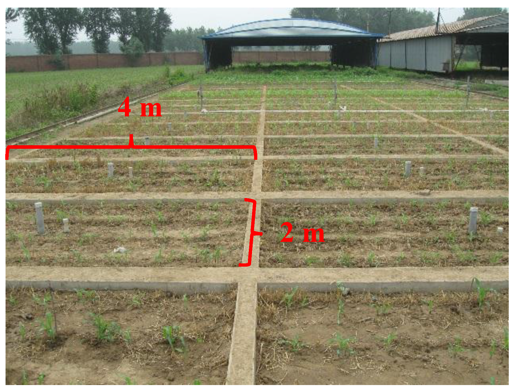
2.2. Experimental Design and Treatments

| Year | Control Plot | Treat. 1 | Treat. 2 | Treat. 3 | Treat. 4 | Treat. 5 | Treat. 6 | Treat. 7 | Field Control |
|---|---|---|---|---|---|---|---|---|---|
| 2013 | 0 | 120 + 80 | 100 + 40 | 80 | 60 | 40 | 25 | 15 | 0 |
| 2014 | 0 | 225 | 150 | 120 | 90 | 60 | 30 | 10 | - |
2.3. Field Measurements
2.3.1. Canopy Spectral Reflectance
| Year | NO. 1 | NO. 2 | NO. 3 | NO. 4 | NO. 5 | NO. 6 | NO. 7 | NO. 8 |
|---|---|---|---|---|---|---|---|---|
| 2013 | 23 July | 30 July | 8 August | 18 August | 25 August | 5 September | 20 September | 8 October |
| 2014 | 10 July | 18 July | 1 August | 7 August | 19 August | 3 September | 16 September | 27 September |
2.3.2. CWC
2.3.3. Soil Water Content
2.4. Vegetation Indices Used in This Analysis
| Index | Equation | Reference |
|---|---|---|
| Normalized difference vegetation index (NDVI) | (ρnir – ρred)/(ρnir + ρred) | [36] |
| Red edge normalized ratio (NRred edge) | (ρ750 – ρ710)/(ρ750 + ρ710) | [37] |
| Water index (WI) | ρ900/ρ970 | [4] |
| Normalized difference water index (NDWI) | (ρ860 – ρ1240)/(ρ860 + ρ1240) | [38] |
| Land surface water index (LSWI) | (ρnir – ρswir)/(ρnir + ρswir) | [39,40] |
| Green chlorophyll index (CIgreen) | (ρ750/ρ550)–1 | [19] |
| Red edge chlorophyll index (CIred edge) | (ρ750/ρ710)–1 | [19] |
| Normalized red edge reflectance curve area (680–780nm; Area680–780) | [41] | |
| Normalized reflectance curve area (1015–1050nm; Area1015–1050) | This study | |
| Normalized reflectance curve area (1110–1170nm; Area1110–1170) | This study |
2.4.1. Normalized Indices
2.4.2. Water-Related Indices
2.4.3. Chlorophyll Indices
2.4.4. Normalized Reflectance Curve Area Indices
3. Results
3.1. Temporal Variations of Soil Moisture, CWC and

| Canopy Biophysical Characteristics | Year | Range (Min–Max) | Mean | Median | SEM | Std. Deviation | CV |
|---|---|---|---|---|---|---|---|
| LAI (leaf area index) | 2013 | 0.23–3.60 | 1.75 | 1.89 | 0.11 | 0.95 | 0.54 |
| 2014 | 0.06–2.78 | 0.89 | 0.75 | 0.09 | 0.71 | 0.80 | |
| FW (fresh weight, g∙m−2) | 2013 | 44.3–917.2 | 412.2 | 414.8 | 27.9 | 236.5 | 0.57 |
| 2014 | 12.7–668.7 | 186.0 | 143.8 | 20.0 | 160.3 | 0.86 | |
| DW (dry weight, g∙m−2) | 2013 | 7.2–206.8 | 91.2 | 95.7 | 6.5 | 55.3 | 0.61 |
| 2014 | 3.3–174.3 | 46.5 | 35.6 | 5.2 | 41.3 | 0.89 | |
| (mean leaf equivalent water thickness at canopy level, g∙cm−2) | 2013 | 0.014–0.026 | 0.018 | 0.018 | 0.00028 | 0.0024 | 0.13 |
| 2014 | 0.010–0.023 | 0.016 | 0.016 | 0.00039 | 0.0032 | 0.20 | |
| CWC (canopy water content, g∙m−2) | 2013 | 36.9–761.4 | 320.9 | 322.2 | 21.7 | 183.7 | 0.58 |
| 2014 | 9.4–494.4 | 139.5 | 105.3 | 15.0 | 119.7 | 0.86 |
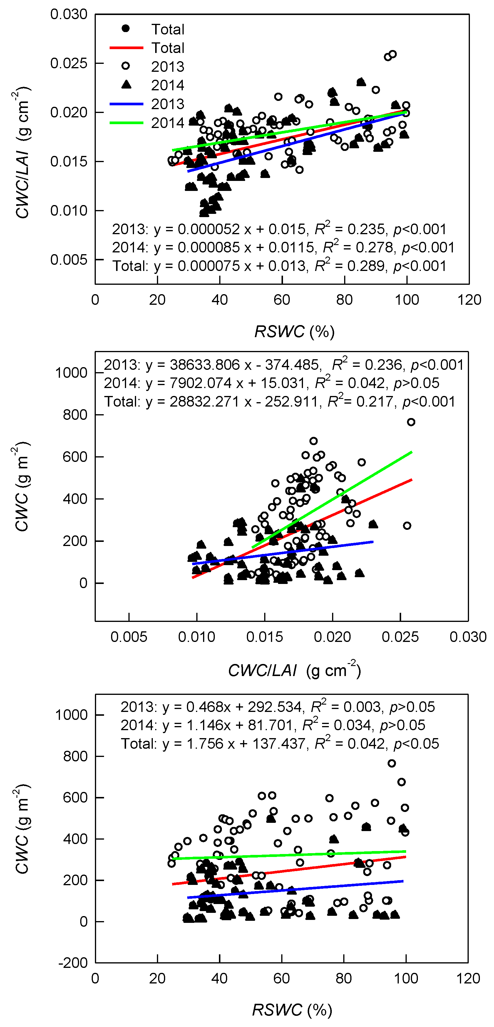
3.2. Relationships between CWC, and Biophysical Properties and RSWC
| RSWC (Relative Soil Water Content, %) | LAI | FW | DW | ||
|---|---|---|---|---|---|
| 2013 (n = 72) | |||||
| (mean leaf equivalent water thickness at canopy level, g cm−2) | 0.441 *** | ||||
| LAI (leaf area index) | −0.054 | 0.360 ** | |||
| FW (fresh weight, g m−2) | 0.027 | 0.472 *** | 0.984 *** | ||
| DW (dry weight, g m−2) | −0.078 | 0.347 ** | 0.962 *** | 0.963 *** | |
| CWC (canopy water content, g m−2) | 0.046 | 0.514 *** | 0.977 *** | 0.997 *** | 0.944 *** |
| 2014 (n = 64) | |||||
| (mean leaf equivalent water thickness at canopy level, g cm−2) | 0.513 *** | ||||
| LAI (leaf area index) | 0.030 | −0.048 | |||
| FW (fresh weight, g m−2) | 0.113 | 0.126 | 0.977 *** | ||
| DW (dry weight, g m−2) | 0.015 | 0.027 | 0.988 *** | 0.987 *** | |
| CWC (canopy water content, g m−2) | 0.143 | 0.156 | 0.970 *** | 0.998 *** | 0.978 *** |
| Total (n = 136) | |||||
| (mean leaf equivalent water thickness at canopy level, g cm−2) | 0.525 *** | ||||
| LAI (leaf area index) | 0.054 | 0.317 *** | |||
| FW (fresh weight, g m−2) | 0.126 | 0.438 *** | 0.987 *** | ||
| DW (dry weight, g m−2) | 0.027 | 0.333 *** | 0.981 *** | 0.980 *** | |
| CWC (canopy water content, g m−2) | 0.153 | 0.466 *** | 0.981 *** | 0.998 *** | 0.969 *** |
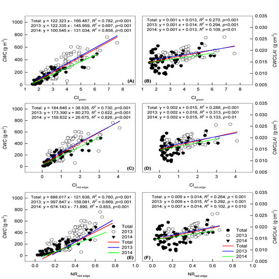
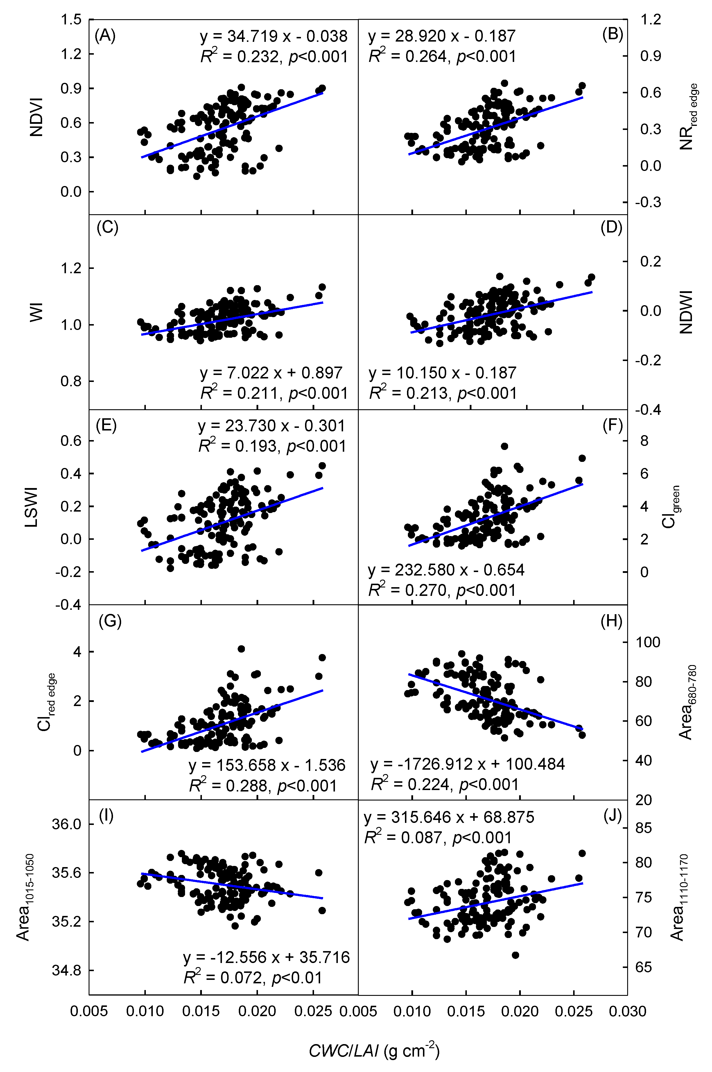
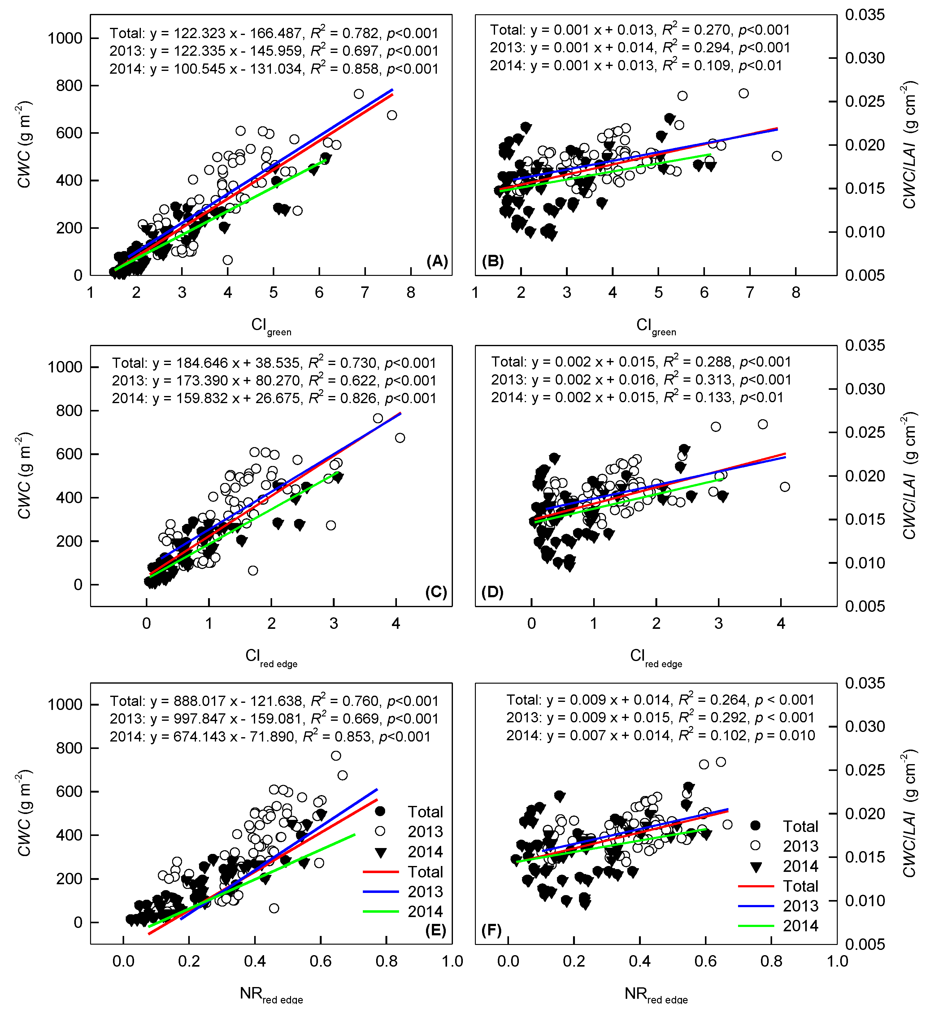
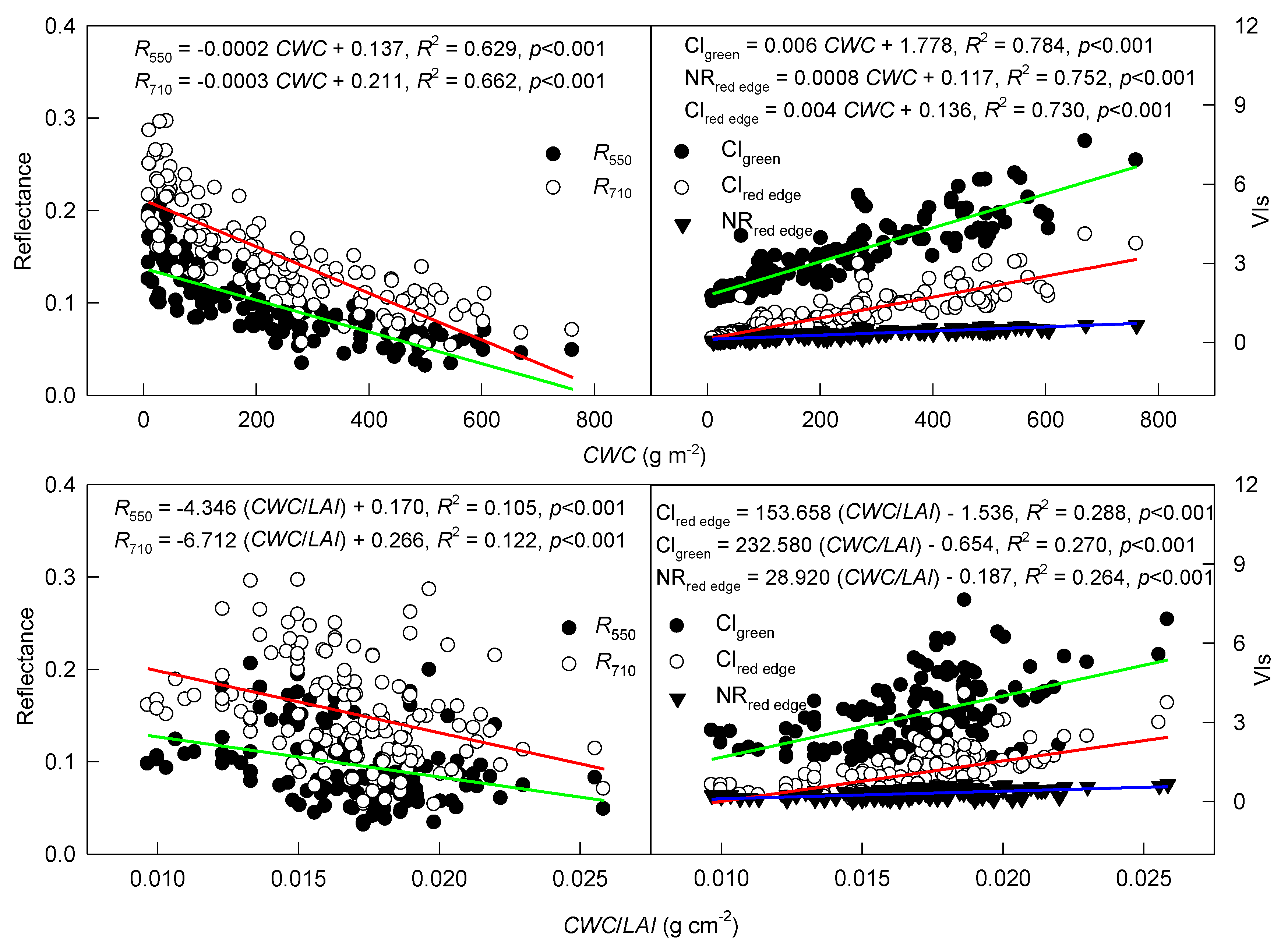
3.3. Relationships between CWC, and VIs


4. Discussion
4.1. Relationships between CWC and and Soil Moisture

4.2. Effects of Different Years on the Relationships between VIs with CWC and

4.3. Performance of Various Indices for Indicating CWC and

5. Conclusions
Acknowledgements
Author Contributions
Conflicts of Interest
References
- Carter, G.A. Responses of leaf spectral reflectance to plant stress. Am. J. Bot. 1993, 80, 239–243. [Google Scholar] [CrossRef]
- Peñuelas, J.; Gamon, J.A.; Fredeen, A.L.; Merino, J.; Field, C.B. Reflectance indices associated with physiological changes in nitrogen and water limited sunflower leaves. Remote Sens. Environ. 1994, 48, 135–146. [Google Scholar] [CrossRef]
- Stimson, H.C.; Breshears, D.D.; Ustin, S.L.; Kefauver, S.C. Spectral sensing of foliar water conditions in two co-occurring conifer species: Pinus edulis and Juniperus monosperma. Remote Sens. Environ. 2005, 96, 108–118. [Google Scholar] [CrossRef]
- Peñuelas, J.; Filella, I.; Biel, C.; Serrano, L.; Save, R. The reflectance at the 950–970 nm region as an indicator of plant water status. Int. J. Remote Sens. 1993, 14, 1887–1905. [Google Scholar] [CrossRef]
- Yi, Q.; Wang, F.; Bao, A.; Jiapaer, G. Leaf and canopy water content estimation in cotton using hyperspectral indices and radiative transfer models. Int. J. Appl. Earth Obs. 2014, 33, 67–75. [Google Scholar] [CrossRef]
- Clevers, J.G.P.W.; Kooistra, L.; Schaepman, M.E. Using spectral information from the NIR water absorption features for the retrieval of canopy water content. Int. J. Appl. Earth Obs. 2008, 10, 388–397. [Google Scholar] [CrossRef]
- Rollin, E.M.; Milton, E.J. Processing of high spectral resolution reflectance data for the retrieval of canopy water content information. Remote Sens. Environ. 1998, 65, 86–92. [Google Scholar] [CrossRef]
- Running, S.W.; Gower, S.T. Forest-BGC, a general model of forest ecosystem processes for regional applications II. Dynamic carbon allocation and nitrogen budgets. Tree Physiol. 1991, 9, 147–160. [Google Scholar] [CrossRef] [PubMed]
- Running, S.W.; Nemani, R.R. Regional hydrologic and carbon balance responses of forests resulting from potential climate change. Climatic Change 1991, 19, 349–368. [Google Scholar] [CrossRef]
- De Jong, S.M.; Addink, E.A.; Doelman, J.C. Detecting leaf-water content in Mediterranean trees using high-resolution spectrometry. Int. J. Appl. Earth Obs. 2014, 27, 128–136. [Google Scholar] [CrossRef]
- Ustin, S.L.; Roberts, D.A.; Gamon, J.A.; Asner, G.P.; Green, R.O. Using imaging spectroscopy to study ecosystem processes and properties. BioScience 2004, 54, 523–534. [Google Scholar] [CrossRef]
- Chuvieco, E.; Rianõ, D.; Aguado, I.; Cocero, D. Estimation of fuel moisture content from multi temporal analysis of Landsat Thematic Mapper reflectance data: Applications in fire danger assessment. Int. J. Remote Sens. 2002, 23, 2145–2162. [Google Scholar] [CrossRef]
- Yilmaz, M.T.; Hunt, E.R., Jr.; Goins, L.D.; Ustin, S.L.; Vanderbilt, V.C.; Jackson, T.J. Vegetation water content during SMEX04 from ground data and Landsat 5 Thematic Mapper imagery. Remote Sens. Environ. 2008, 112, 350–362. [Google Scholar] [CrossRef]
- Gitelson, A.A.; Viña, A.; Arkebauer, T.J.; Rundquist, D.C.; Keydan, G.; Leavitt, B. Remote estimation of leaf area index and green leaf biomass in maize canopies. Geophys. Res. Lett. 2003, 30. [Google Scholar] [CrossRef]
- Viña, A.; Gitelson, A.A.; Nguy-Robertson, A.L.; Peng, Y. Comparison of different vegetation indices for the remote assessment of green leaf area index of crops. Remote Sens. Environ. 2011, 115, 3468–3478. [Google Scholar] [CrossRef]
- Nguy-Robertson, A.L.; Peng, Y.; Gitelson, A.A.; Arkebauer, T.J.; Pimstein, A.; Herrmann, I.; Karnieli, A.; Rundquist, D.C.; Bonfil, D.J. Estimating green LAI in four crops: Potential of determining optimal spectral bands for a universal algorithm. Agric. For. Meteorol. 2014, 192, 140–148. [Google Scholar] [CrossRef]
- Viña, A.; Gitelson, A.A. New developments in the remote estimation of the fraction of absorbed photosynthetically active radiation in crops. Geophys. Res. Lett. 2005, 32. [Google Scholar] [CrossRef]
- Zhang, F.; Zhou, G.; Nilsson, C. Remote estimation of the fraction of absorbed photosynthetically active radiation for a maize canopy in Northeast China. J. Plant Ecol. 2015, 8, 429–435. [Google Scholar] [CrossRef]
- Gitelson, A.A.; Viña, A.; Ciganda, V.; Rundquist, D.C.; Arkebauer, T.J. Remote estimation of canopy chlorophyll content in crops. Geophys. Res. Lett. 2005, 32. [Google Scholar] [CrossRef]
- Wu, C.; Niu, Z.; Tang, Q.; Huang, W. Estimating chlorophyll content from hyperspectral vegetation indices: Modeling and validation. Agric. For. Meteorol. 2008, 148, 1230–1241. [Google Scholar] [CrossRef]
- Wu, C.; Niu, Z.; Tang, Q.; Huang, W.; Rivard, B.; Feng, J. Remote estimation of gross primary production in wheat using chlorophyll-related vegetation indices. Agric. For. Meteorol. 2009, 149, 1015–1021. [Google Scholar] [CrossRef]
- Peng, Y.; Gitelson, A.A. Application of chlorophyll-related vegetation indices for remote estimation of maize productivity. Agric. For. Meteorol. 2011, 151, 1267–1276. [Google Scholar] [CrossRef]
- Zhang, F.; Zhou, G. Estimating canopy photosynthetic parameters in maize field based on multi-spectral remote sensing. Chin. J. Plant Ecol. 2014, 38, 710–719. [Google Scholar]
- Colombo, R.; Meroni, M.; Marchesi, A.; Busetto, L.; Rossini, M.; Giardino, C.; Panigada, C. Estimation of leaf and canopy water content in poplar plantations by means of hyperspectral indices and inverse modeling. Remote Sens. Environ. 2008, 112, 1820–1834. [Google Scholar] [CrossRef]
- Clevers, J.G.P.W.; Kooistra, L.; Schaepman, M.E. Estimating canopy water content using hyperspectral remote sensing data. Int. J. Appl. Earth Obs. 2010, 12, 119–125. [Google Scholar] [CrossRef]
- Mirzaie, M.; Darvishzadeh, R.; Shakiba, A.; Matkan, A.A.; Atzberger, C.; Skidmore, A. Comparative analysis of different uni- and multi-variate methods for estimation of vegetation water content using hyper-spectral measurements. Int. J. Appl. Earth Obs. 2014, 26, 1–11. [Google Scholar] [CrossRef]
- Darvishzadeh, R.; Atzberger, C.; Skidmore, A.; Schlerf, M. Mapping grassland leaf area index with airborne hyperspectral imagery: A comparison study of statistical approaches and inversion of radiative transfer models. ISPRS J. Photogramm. Remote Sens. 2011, 66, 894–906. [Google Scholar] [CrossRef]
- Atzberger, C.; Darvishzadeh, R.; Immitzer, M.; Schlerf, M.; Skidmore, A.; Le Maire, G. Comparative analysis of different retrieval methods for mapping grassland leaf area index using airborne imaging spectroscopy. Int. J. Appl. Earth Obs. 2015, 43, 19–31. [Google Scholar] [CrossRef]
- Zhang, F.; John, R.; Zhou, G.; Shao, C.; Chen, J. Estimating canopy characteristics of Inner Mongolia’s grasslands from field spectrometry. Remote Sens. 2014, 6, 2239–2254. [Google Scholar] [CrossRef]
- Atzberger, C.; Guérif, M.; Baret, F.; Werner, W. Comparative analysis of three chemometric techniques for the spectroradiometric assessment of canopy chlorophyll content in winter wheat. Comput. Electron. Agr. 2010, 73, 165–173. [Google Scholar] [CrossRef]
- Ren, H.; Zhou, G. Estimating aboveground green biomass in desert steppe using band depth indices. Biosyst. Eng. 2014, 127, 67–78. [Google Scholar] [CrossRef]
- Tan, K.; Zhou, G.; Ren, S. Response of leaf dark respiration of winter wheat to changes in CO2 concentration and temperature. Chin. Sci. Bull. 2013, 58. [Google Scholar] [CrossRef]
- Li, B. Maize Drought Process and Its Dynamics Simulation. Master’s Thesis, Chinese Academy of Meteorological Sciences, Beijing, China, 2014. [Google Scholar]
- Ceccato, P.; Gobron, N.; Flasse, S.; Pinty, B.; Tarantola, S. Designing a spectral index to estimate vegetation water content from remote sensing data: Part 1—Theoretical approach. Remote Sens. Environ. 2002, 82, 188–197. [Google Scholar] [CrossRef]
- Danson, F.M.; Steven, M.D.; Malthus, T.J.; Clark, J.A. High-spectral resolution data for determining leaf water content. Int. J. Remote Sens. 1992, 13, 461–470. [Google Scholar] [CrossRef]
- Rouse, J.W.; Haas, R.H., Jr.; Schell, J.A.; Deering, D.W. Monitoring the Vernal Advancement and Retrogradation (Green Wave Effect) of Natural Vegetation; Progress Report RSC 1978-1; Remote Sensing Center, Texas A&M University: College Station, TX, USA, 1973. [Google Scholar]
- Gitelson, A.A.; Merzlyak, M.N. Signature analysis of leaf reflectance spectra: Algorithm development for remote sensing. J. Plant Physiol. 1996, 148, 493–500. [Google Scholar] [CrossRef]
- Gao, B.C. NDWI—A normalized difference water index for remote sensing of vegetation liquid water from space. Remote Sens. Environ. 1996, 58, 257–266. [Google Scholar] [CrossRef]
- Jurgens, C. The modified normalized difference vegetation index (mNDVI)—A new index to determine frost damages in agriculture based on Landsat TM data. Int. J. Remote Sens. 1997, 18, 3583–3594. [Google Scholar] [CrossRef]
- Xiao, X.; Boles, S.; Liu, J.; Zhuang, D.; Frolking, S.; Li, C.; Salas, W.; Moore, B. Mapping paddy rice agriculture in southern China using multi-temporal MODIS images. Remote Sens. Environ. 2005, 95, 480–492. [Google Scholar] [CrossRef]
- Ren, H.; Zhou, G.; Zhang, X. Estimation of green aboveground biomass of desert steppe in Inner Mongolia based on red-edge reflectance curve area method. Biosyst. Eng. 2011, 109, 385–395. [Google Scholar] [CrossRef]
- Gitelson, A.A.; Merzlyak, M. Spectral reflectance changes associated with autumn senescence of Asculus hippocastanum and Acer platanoides leaves: Spectral features and relation to chlorophyll estimation. J. Plant Physiol. 1994, 143, 286–292. [Google Scholar] [CrossRef]
- Gitelson, A.A.; Viña, A.; Verma, S.B.; Rundquist, D.C.; Arkebauer, T.J.; Keydan, G.; Leavitt, B.; Ciganda, V.; Burba, G.G.; Suyker, A.E. Relationship between gross primary production and chlorophyll content in crops: Implications for the synoptic monitoring of vegetation productivity. J. Geophys. Res. 2006, 111. [Google Scholar] [CrossRef]
- Curran, P.J. Remote sensing of foliar chemistry. Remote Sens. Environ. 1989, 30, 271–278. [Google Scholar] [CrossRef]
© 2015 by the authors; licensee MDPI, Basel, Switzerland. This article is an open access article distributed under the terms and conditions of the Creative Commons Attribution license (http://creativecommons.org/licenses/by/4.0/).
Share and Cite
Zhang, F.; Zhou, G. Estimation of Canopy Water Content by Means of Hyperspectral Indices Based on Drought Stress Gradient Experiments of Maize in the North Plain China. Remote Sens. 2015, 7, 15203-15223. https://0-doi-org.brum.beds.ac.uk/10.3390/rs71115203
Zhang F, Zhou G. Estimation of Canopy Water Content by Means of Hyperspectral Indices Based on Drought Stress Gradient Experiments of Maize in the North Plain China. Remote Sensing. 2015; 7(11):15203-15223. https://0-doi-org.brum.beds.ac.uk/10.3390/rs71115203
Chicago/Turabian StyleZhang, Feng, and Guangsheng Zhou. 2015. "Estimation of Canopy Water Content by Means of Hyperspectral Indices Based on Drought Stress Gradient Experiments of Maize in the North Plain China" Remote Sensing 7, no. 11: 15203-15223. https://0-doi-org.brum.beds.ac.uk/10.3390/rs71115203