Mapping Cropland in Smallholder-Dominated Savannas: Integrating Remote Sensing Techniques and Probabilistic Modeling

Abstract

Traditional smallholder farming systems dominate the savanna range countries of sub-Saharan Africa and provide the foundation for the region’s food security. Despite continued expansion of smallholder farming into the surrounding savanna landscapes, food insecurity in the region persists. Central to the monitoring of food security in these countries, and to understanding the processes behind it, are reliable, high-quality datasets of cultivated land. Remote sensing has been frequently used for this purpose but distinguishing crops under certain stages of growth from savanna woodlands has remained a major challenge. Yet, crop production in dryland ecosystems is most vulnerable to seasonal climate variability, amplifying the need for high quality products showing the distribution and extent of cropland. The key objective in this analysis is the development of a classification protocol for African savanna landscapes, emphasizing the delineation of cropland. We integrate remote sensing techniques with probabilistic modeling into an innovative workflow. We present summary results for this methodology applied to a land cover classification of Zambia’s Southern Province. Five primary land cover categories are classified for the study area, producing an overall map accuracy of 88.18%. Omission error within the cropland class is 12.11% and commission error 9.76%.

1. Introduction

Savanna biomes cover roughly one-fifth of the planet’s terrestrial surface with the largest spatial extents found in sub-Saharan Africa. Among the savanna-range countries, agricultural activity constitutes a large segment of the economic sector, employing 70% of labor and accounting for 32% of GDP [1]. Traditional smallholder farming systems dominate the agricultural landscape where smallholders play an integral part in shaping the socioeconomic and ecological fabric of the region and provide the foundation for food security. Despite increasing agricultural production over the last 30 years, yield has not kept pace with exponential population growth and food insecurity remains prevalent [2]. The response of cultivating more land to increase productivity has put savannas under intense pressure [3,4] with little improvement in yield [2]. To meet the rapidly growing food demands of the projected doubling of the region’s population by 2050 [5], and the growing interest in using the capacity for additional cropland to enhance economic development in the region [6,7], conversion of savanna to cropland is expected to continue at an advancing pace. In addition to this concern, this region’s high climate variability, and vulnerability to drought, pose a significant and increasing risk to agriculturally-based livelihoods [8,9]. A mechanism that can support the monitoring and assessment of food security and improve understanding of how climate variability affects regional crop production could offer a valuable tool to the region.

Reliable cropland maps are fundamental to informing both local and global development and natural resource management policies [6], being an essential input for evaluating food security, land use/land cover dynamics, investment priorities, conservation policies, and a host of other factors [10,11,12]. Yet, there is little agreement of the cropland baseline, reflected by the lack of consensus among regional and global land cover products. Global estimates of total cropland area differ by as much as 40% [13], and estimates within semi-arid regions of Africa have even greater uncertainty, largely attributable to the difficulty of mapping cropland in smallholder systems [12,14].

This difficulty is pronounced in savannas, where smallholder systems predominate, and the characteristics of savanna vegetation make it particularly hard to distinguish from small-scale farms. Smallholders use low intensity practices to cultivate small fields, and often preserve large fruit-bearing trees within their field boundaries [15]. The combination of field size, residual tree canopies, and crop diversity magnify the within-class variability of crop field while blurring the spectral distinction between croplands and savannas. The difficulty in distinguishing cropland from savanna is evidenced by the disagreement between products derived from remote sensing and statistical inventories of African agriculture [16,17]. Given these discrepancies, and the absence of a single reliable dataset to inform policy decisions regarding food security issues and land use, an effective and rigorous methodology for mapping croplands from satellite images is much needed for sub-Saharan savanna landscapes [18].

1.1. Objectives

In this paper, we integrate remote sensing techniques of classification and error detection with logistic regression into an innovative workflow. Although we categorize multiple primary land covers, the key objective is the development of a classification protocol to effectively capture cropland in a savanna landscape. The workflow combines statistical clustering, supervised classification, proportional sampling, and targeted error detection with a probabilistic reclassification technique (logit models), incorporating elements of phenology and physically-based fraction estimates of land cover. While the set of analytical techniques utilized here has been part of the existing toolkit of remote sensing researchers, the innovation in this approach is the combination of sequence and strict application of techniques. We demonstrate this methodology with results derived from a land cover classification of the smallholder-dominated, semi-arid province of Southern Zambia. Land cover is classified into five primary categories over a study area covered by three adjacent Landsat 5 Thematic Mapper (TM) footprints, producing an overall accuracy of 88.18% and reducing errors of omission and commission within the cropland class to 12% and 10% respectively.

Policy analysts and practitioners note that satellite-derived measures of cropland in Africa, with minimum accuracies ranging between 80 and 85 percent, could fill in statistical data gaps and provide valuable data for designing development programs and targeting donor investment, as well as “monitoring dynamics of agriculture extent and output and evaluating food security in the continent” [18,19]. The classification protocol we present in this paper is a practical, flexible, and effective approach to cropland mapping in a smallholder savanna environment. It has the potential to provide a valuable accounting and decision-making tool, essential for the sustainable agricultural development, food security, and ecosystem service provisioning of savanna range countries in Africa.

1.2. Review of Techniques for Remote Sensing Cropland in Savanna Landscapes

Savannas are common ecosystems that are distributed globally across the tropic and sub-tropic latitudes. Comprised of grasslands interspersed with bushes and trees in varying densities, savannas provide essential services in the form of carbon storage and climate regulation, and habitat for many mega-fauna species [20]. A variety of remote sensing approaches have been proposed to map cropland within savanna landscapes. In the Brazilian Cerrado, land cover was classified into discrete map categories, including pasture and cropland, by applying a random forest classifier to Landsat derived spectral-temporal statistical metrics [21]. The temporal window of Landsat data used in this study spanned a period of several years. This method achieved an overall accuracy of 92%, but the temporal depth of 3 years may prohibit the use of this approach in locations where savannas are undergoing rapid conversion and more frequent monitoring is desired, such as those on the African continent. Estes et al. [22] applied support vector machines (SVM) to temporal Landsat data in a classification of the greater Serengeti ecosystem, achieving high accuracies for both stable and conversion categories, however, the approach poses some potential challenges related to training and validating the conversion category, notably the reliable identification of converted area and the directionality of conversion.

Temporal measures of the Normalized Difference Vegetation Index (NDVI), coupled with mono-temporal refinement techniques, have also been utilized in a supervised land cover classification of a marginal semi-arid region within the Sahelian belt of Niger [23]. Omission and commission errors were 5% and 12% respectively for the cultivated category, but this success is largely dependent on having images available throughout the entire season. In addition to issues related to data availability, using NDVI in savannas can be problematic given that the index is affected by soil color and scale [24,25,26,27,28].

Object-based classifiers (OBC) have received increasing attention because of their ability to incorporate spatial data into the classification process. Utilized in conjunction with high resolution satellite data, OBCs have been used to identify cropland [29] and to differentiate woodland from surrounding land cover in a savanna environment [30]. However, research has shown the only significant advantage of an OBC over a maximum likelihood classifier (MLC) is discriminating vegetation classes with complex forest stand structures [31]. Additionally, cost and data storage are significant logistical challenges, particularly when the spatial extent of a study area is large.

Results from other remote sensing studies in semi-arid environments suggest that fraction cover estimates made using unmixing methods are less affected by soil background than NDVI [32,33,34,35,36,37].There are several methods for estimating sub-pixel fractions of land cover, including multi-resolution approaches and spectral mixture analysis (SMA). Gessner et al. [38] introduced a method of scaling up from an initial classification of high-resolution data to medium and coarse resolution imagery through a process of sampling and the use of random forest regression trees. A major limitation of this method is that the requisite high-resolution data are often unavailable.

SMA estimates the fractional composition of land cover within a pixel by using the spectral signatures of endmembers, or “pure pixels” [39], treating a pixel’s spectrum as a linear combination of the spectra of its physical elements [40]. Spectral unmixing has been suggested to be among the most promising techniques for obtaining data on surface cover in savanna environments where there is a large presence of non-photosynthetic vegetation (NPV), and reflectance is affected by scattering, mixing, and variability in soil composition [34]. The technique has been recommended for semi-arid study sites where there is a high frequency of mixed pixels and reflectance is dominated by the soil background [35]. Research has shown that a basic three-endmember spectral mixture model can represent over 95% of all observed Landsat image spectra, producing fraction estimates that closely agree with in situ measurements and quantitative output that directly relates to the physical characteristics of land cover [41]. Spectral unmixing has been effectively applied to both mono and multi-temporal data in semi-arid environments in monitoring desertification and desertification risk [42,43], rangeland degradation [44], and mapping invasive grasses [45].

Logistic regression is a flexible alternative to the traditional supervised classification approach. Hogland et al. (2013) [46] discuss the “desirable qualities” of logistic regression underscoring the rather unrestrictive model assumptions, the model’s incorporation of both categorical and continuous variables into the classification scheme, ease of model comparisons, and a focus on direct modeling of class probabilities. Environmental variables have been paired with logistic regression to identify distributions of land cover [47] but coupled with multispectral data and derivatives, logistic regression has been utilized to classify land cover [48], identify areas of advancing land degradation [49], and mapped burned lands [50]. We adopt logistic regression in the classification protocol presented here, pairing the logit model with multispectral derivatives generated from temporal intra-band differencing and spectral unmixing.

2. Data and Methods

2.1. Study Area

Zambia is a nation with an extensive land resource base (58% classified as arable), much of it covered by savanna and savanna woodland, and possessing 40% of the water in Central and Southern Africa [51,52]. With only 14% of the resource base cultivated each year, and the agriculture sector accounting for almost 70% of labor force employment, Zambia is one of the global focal points for agricultural expansion [53]. The Southern Province of Zambia (Figure 1) is one of the key agricultural regions in the country. The province falls within the semi-arid/highland semi-arid agro-ecological zones and is dominated by smallholder farming, similar to the Central, Lusaka, and Eastern provinces of Zambia and comparable regions in south-central Africa, the Sahel, and east African steppe. The climate is sub-tropical, characterized by three seasons: cool dry (April–August), hot dry (August–November), and warm wet season (November-April). Average temperatures are between 14 °C and 28 °C with an average annual rainfall accumulation of 800–1000 mm (less than 700mm in the South Chama and Lundazi regions of the extreme south). The province is dominated by clay soils supporting primary crops of maize, cassava, groundnuts, millet, seed cotton, and wheat. The population was estimated to be over 880,000 in 2010, an increase of approximately 38% from 1990 [54].

Figure 1. Country of Zambia with provinces outlined in black and water bodies/seasonally inundated areas in blue. The Southern Province is highlighted in green.

Figure 1. Country of Zambia with provinces outlined in black and water bodies/seasonally inundated areas in blue. The Southern Province is highlighted in green.

2.2. Data

Landsat 5 Thematic Mapper (TM) data was collected for three footprints that covered nine of eleven administrative districts, either wholly or in large part. The footprints were located at nominal scene centers of Path: 172, Row: 071; Path: 172, Row: 072; and Path: 173, Row: 071. Given the breadth of study area and characteristic smallholder farming, the Landsat 5 TM instrument offered the optimal pixel resolution of 30 m [55]. Two images were selected for each satellite footprint with acquisition dates corresponding to the pre-season of 2008 and the harvest season of 2009 (

Table A1. TM scene acquisition dates for each of three footprints classified.

Footprint (WRS2)	Pre-Season Date	Harvest Season Date
Path: 172; Row: 071	26 September 2008	24 May 2009
Path: 172; Row: 072	26 September 2008	24 May 2009
Path: 173; Row: 071	3 October 2008	31 May 2009

). The choice of 2008/2009 imagery coincided with survey data collected during 2007–2008. Optimally, scenes from the growing season would also be utilized but persistent heavy cloud cover combined with the 16-day reacquisition interval did not yield an image of sufficient quality. Quantized calibrated pixel values were converted to at-sensor radiance based on the minimum and maximum spectral radiance for each band [56]. Radiance values were subsequently converted to surface reflectance using an image-based procedure of dark-object subtraction [57,58]. Fmask software (https://code.google.com/p/fmask/) was utilized to identify cloud/heavy haze and cloud shadow in each TM scene. Cloud masks were combined into a cumulative mask and applied to both images. Multi-temporal composites were then generated for each footprint by stacking the six multi-spectral bands (TM 1–5, and 7) of the seasonal image pairs to generate a 12-layer image.

2.3. Analysis

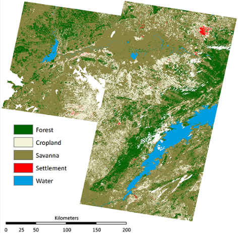
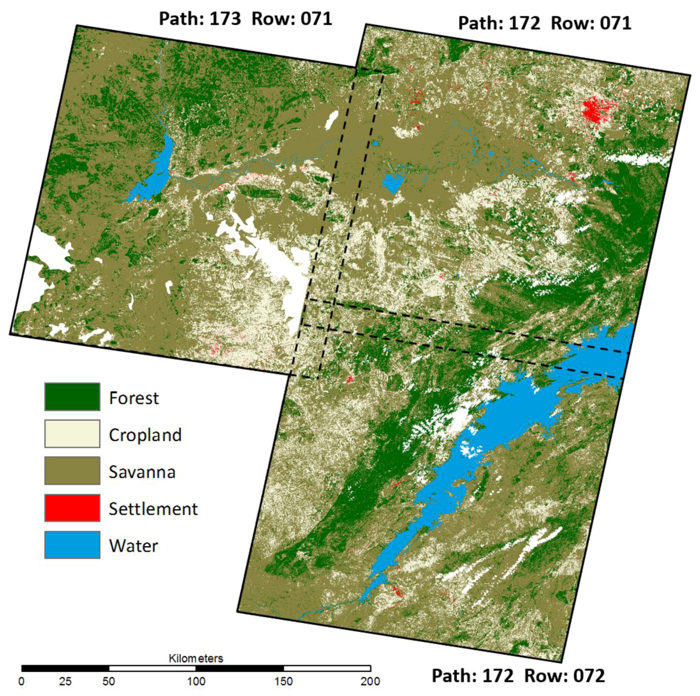
Given the slight differences in image acquisition dates, and inherent difficulties related to normalizing reflectance among adjacent scenes, each footprint was classified independently. Land cover within the area delineated by the TM footprint at Path: 172; Row: 071 (WRS 2) was classified first. The method for classifying land cover in this footprint, and classification results, are presented in detail. Classification results from the two adjacent footprints are provided in the supplement.

To develop a training dataset, a clustering algorithm (ISODATA) in Erdas IMAGINE was applied to the multi-temporal spectral data to identify statistical patterns and segment pixels into natural occurring clusters. Utilizing a minimum spectral distance formula, pixels were grouped into ten clusters and randomly sampled, generating 75 points within each unsupervised cluster. Square buffers, delineating an area of 900 m², were constructed around sample points and a ground cover label assigned to each polygon through interpretation of high resolution Google Earth imagery [22,59,60]. Training locations were coded with Google Earth imagery acquired between 2007 and 2010. Of the total sample of 750 points, 498 were interpretable and intersected with suitable land cover reference imagery. Training data were labeled as 1 of 5 primary land cover classes: (1) forest; (2) cropland; (3) savanna; (4) settlement; and (5) water. The dominant land covers were adequately sampled by this scheme, however, the settlement class was underrepresented so purposeful sampling was performed to supplement the training data for that category with an additional 25 points.

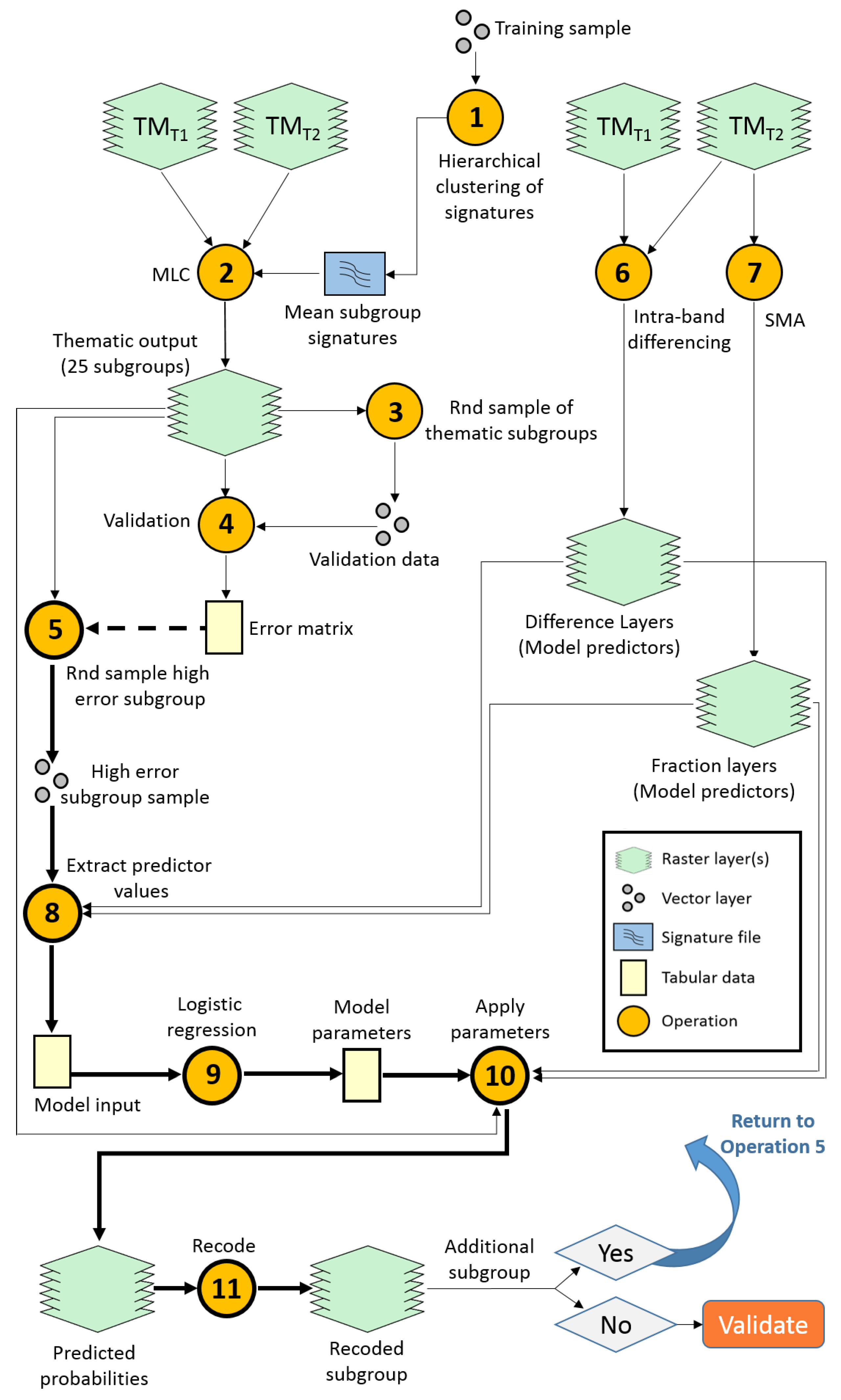
A processing diagram is provided to illustrate the workflow that follows (Figure 2). As operations are described, text is provided directing to specific points in the diagram, e.g., “Operation 1, Figure 2” refers to the operation icon in the workflow labeled “1” (hierarchical clustering of training signatures). Spectral signatures were extracted from the multi-temporal data at sample locations and imported into DataDesk statistical software [61]. Because intra-class spectral variability was high, the compliment of signatures associated with each primary land cover category was grouped into spectrally similar subsets, or subgroups, using hierarchical clustering (Operation 1, Figure 2). Mean subgroup signatures were produced by averaging signature values for each unique cluster of signatures.

Figure 2. Classification workflow using objects and syntax analogous to the model builder in ERDAS Imagine. Note that reclassification iterations are performed by repeating the loop of Operations 5, 8–11 (in bold), the remaining operations are performed once. The dashed line, directing to Operation 5 in the diagram, represents data not used directly in the operation but rather to establish parameters for Operation 5.

Figure 2. Classification workflow using objects and syntax analogous to the model builder in ERDAS Imagine. Note that reclassification iterations are performed by repeating the loop of Operations 5, 8–11 (in bold), the remaining operations are performed once. The dashed line, directing to Operation 5 in the diagram, represents data not used directly in the operation but rather to establish parameters for Operation 5.

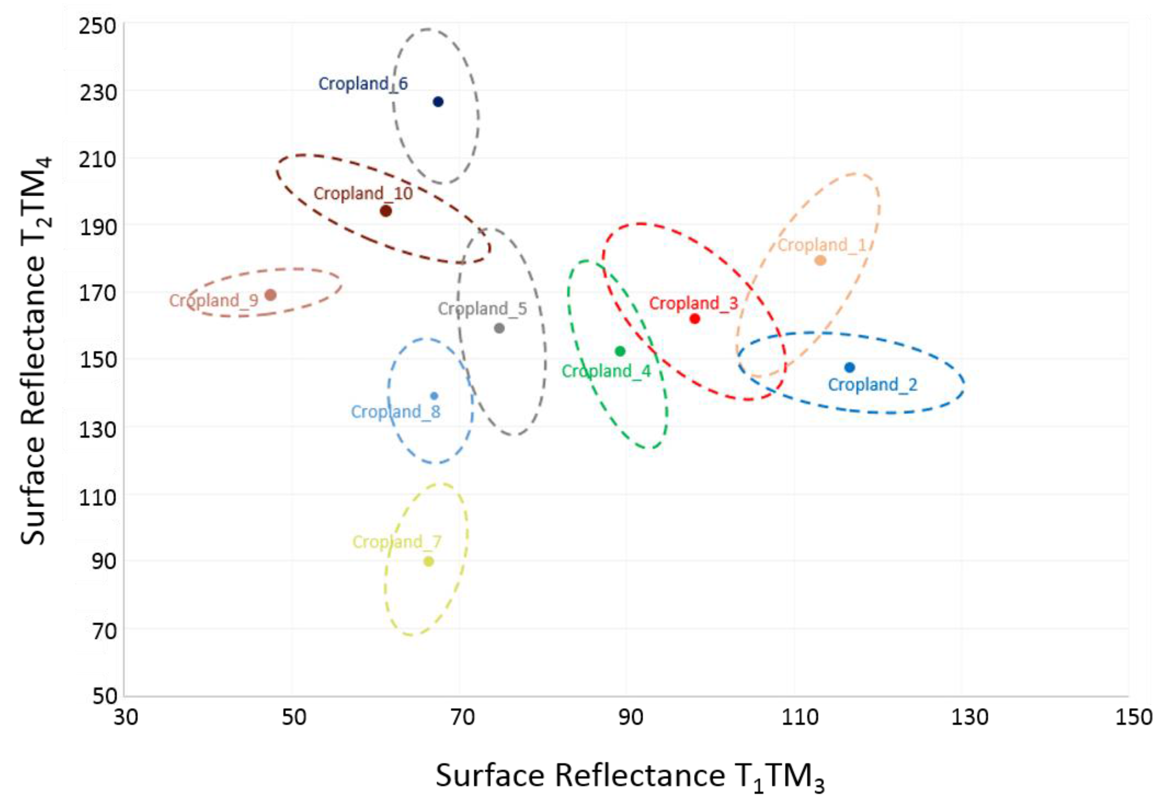
Separability was tested among subgroup signatures, within primary categories, by calculating the Transformed Divergence (TD) [62], merging signature pairs with a TD value less than 1700 [63]. Spectral variability was high among all non-water categories. The greatest variability was observed in the cropland class where spectral signatures were partitioned into 10 clusters with minimal overlap (Figure 3).

Figure 3. Distribution of cropland clusters in T₁TM₃ (x-axis) and T₂TM₄ (y-axis) feature space. Dashed lines delineate the distribution of individual signatures that compose the respective cluster. TM₃ is utilized to illustrate soil reflectance variability and TM₄ to illustrate the variability in vegetation response. Surface reflectance is scaled to unsigned 8-bit.

Figure 3. Distribution of cropland clusters in T₁TM₃ (x-axis) and T₂TM₄ (y-axis) feature space. Dashed lines delineate the distribution of individual signatures that compose the respective cluster. TM₃ is utilized to illustrate soil reflectance variability and TM₄ to illustrate the variability in vegetation response. Surface reflectance is scaled to unsigned 8-bit.

The bulk of training samples (~67%) was distributed among the cropland and savanna categories. Hierarchical clustering of training signatures produced 3 to 10 subgroups for non-water categories with cropland and savanna represented by the greatest number of subgroups (Table 1). The mean signatures used to parameterize the initial classification represented the average spectral value of each of these subgroups. We categorized the spectral data in Erdas IMAGINE with a MLC, selecting all layers in the temporal dataset as input to the classifier and applying the 25 subgroup signatures (Operation 2, Figure 2). The 25-category thematic output serves several purposes, namely: a mechanism for identifying and isolating commission error within spatially defined strata of primary land covers; a sampling template, and, a mask to spatially constrain pixel reclassification. The number of primary categories and breadth of training data dictates the quantity of subgroups and the number of classes in the thematic output. These parameters will vary by type of study and composition of landscape but the method of primary category stratification is certainly generalizable to a variety of studies, and equally, landscapes.

Table 1. Primary category training data for footprint at Path: 172 Row: 071: category description, sample size, and number of subgroups. Column 3 indicates the total number of training samples for each primary category. Column 4 indicates the number of subgroups generated from the hierarchical clustering of training signatures.

Primary LC Category	Description	Sample Size	No. Subgroups
Forest	Tree assemblages ≥ 40% canopy closure	88	5
Cropland	Cultivated land for subsistence or commercial agriculture	177	10
Savanna	Savanna: grassland (woody canopy cover < 10%), bushland savanna (10% < bush cover < 40%), woodland savanna (10% < tree canopy < 40%) [55,56].	172	6
Settlement	Urban areas, villages, and roads	54	3
Water	Lakes, rivers, streams, and seasonally inundated areas	32	1

Table 1. Primary category training data for footprint at Path: 172 Row: 071: category description, sample size, and number of subgroups. Column 3 indicates the total number of training samples for each primary category. Column 4 indicates the number of subgroups generated from the hierarchical clustering of training signatures.

Primary LC Category	Description	Sample Size	No. Subgroups
Forest	Tree assemblages ≥ 40% canopy closure	88	5
Cropland	Cultivated land for subsistence or commercial agriculture	177	10
Savanna	Savanna: grassland (woody canopy cover < 10%), bushland savanna (10% < bush cover < 40%), woodland savanna (10% < tree canopy < 40%) [55,56].	172	6
Settlement	Urban areas, villages, and roads	54	3
Water	Lakes, rivers, streams, and seasonally inundated areas	32	1

Proportional random sampling of the 25-category thematic map was used to generate validation points (Operation 3, Figure 2). A total of 477 validation points were interpretable and intersected with suitable reference land cover imagery. Since classification accuracy in Erdas IMAGINE is evaluated within a 3-pixel by 3-pixel window, square buffers (8100 m²) were constructed around the sample validation points and a land cover label assigned to each polygon through interpretation of Google Earth imagery.

Classification error was evaluated through an accuracy assessment of the 25-category (subgroup) thematic map (Operation 4, Figure 2). The assessment allowed us to examine the distribution of error within strata of a primary category and identify the subgroup(s) where the greatest classification error resided. The largest detected commission errors were related to savanna misclassified as cropland and cropland as settlement. An examination of a portion of the error matrix, revealed error concentrated in the cropland_3 and cropland_4 subgroups and within the settlement_2 and settlement_3 subgroups (Table 2).

Table 2. Partial classification error matrix containing cropland and settlement subgroups. Rows represent the classified subgroup map categories and columns represent reference or validation data. High commission errors are indicated by asterisks.

Subgroup	Forest	Cropland	Savanna	Settlement	Water
Cropland_1	0	27	0	0	0
Cropland_2	0	32	0	0	0
Cropland_3	0	28	13*	0	0
Cropland_4	0	6	28*	0	0
Cropland_5	0	2	0	0	0
Cropland_6	0	1	0	0	0
Cropland_7	0	1	0	0	0
Cropland_8	0	33	0	0	0
Cropland_9	0	4	0	0	0
Cropland_10	0	2	0	0	0
Settlement_1	0	1	0	2	0
Settlement_2	0	8*	0	37	0
Settlement_3	0	7*	0	1	0

Table 2. Partial classification error matrix containing cropland and settlement subgroups. Rows represent the classified subgroup map categories and columns represent reference or validation data. High commission errors are indicated by asterisks.

Subgroup	Forest	Cropland	Savanna	Settlement	Water
Cropland_1	0	27	0	0	0
Cropland_2	0	32	0	0	0
Cropland_3	0	28	13*	0	0
Cropland_4	0	6	28*	0	0
Cropland_5	0	2	0	0	0
Cropland_6	0	1	0	0	0
Cropland_7	0	1	0	0	0
Cropland_8	0	33	0	0	0
Cropland_9	0	4	0	0	0
Cropland_10	0	2	0	0	0
Settlement_1	0	1	0	2	0
Settlement_2	0	8*	0	37	0
Settlement_3	0	7*	0	1	0

Reclassification was iterative, each iteration addressing commission error within a particular high-error subgroup and restricted to the spatial extent of same. There were, overall, five subgroups reclassified within the footprint (Path: 172 Row: 071) but only four subgroups directly affected error in the primary cropland class: two cropland and two settlement. We limit our description of method and models to these subgroups, describing the approach to reclassification in detail using one of the cropland subgroups and one of the settlement groups as examples.

Commission error within the cropland_3 class resulted in 13 known areas of savanna misclassified as cropland (Table 2), indicating a data high degree of spectral confusion between savanna and cropland within this strata. We randomly sampled 200 locations within the cropland_3 thematic subgroup and assigned a land cover label (Operation 5, Figure 2). Land cover was interpreted for 176 observations with high confidence, the remainder were eliminated from the analysis.

The assessment indicated that classification error was distributed between two primary land cover categories (e.g., cropland and savanna) within subgroups; the binary outcome allowed us to use logistic regression to estimate the probability that one of the two particular land covers was present given a set of predictors. The binary logistic regression model has the form:

$$ln\left(\raisebox{1ex}{$p$}\!\left/ \!\raisebox{-1ex}{$\left(1-p\right)$}\right.\right)=a+b_1{x}_1+b_2{x}_2+\mathrm{...}{b}_n{x}_n,$$

(1)

where p = probability of a case belonging to category 1; p/(1 – p) = odds; a = constant; n = number of predictors; b₁...b_n = regression coefficients; and bx₁...x_n = regression predictors.

Logit models are used as the basis for pixel reclassification for a number of reasons. First, logistic regression does not assume a linear relationship between predictors and the outcome variable. Second, accuracy assessment of the subgroup thematic map indicates that the dependent variable is dichotomous. Third, there are no predictor requirements for normality, linearity, or equal variance within primary categories of subgroups. Fourth, the primary categories are mutually exclusive and exhaustive. Last, logit models provide an efficient way of testing classification outcomes and offer a flexible interface for evaluating the contribution of any given predictor, or set of predictors.

Predictors for the logit model were generated from the original multi-spectral data, incorporating elements of phenology and sub-pixel composition of land cover. Multi-temporal data is utilized to capture variability in phenology which has been demonstrated to enhance differentiation between cropland and surrounding natural land cover [59,64,65,66] as well as among crop type [67,68]. Temporal intra-band differencing (e.g., B1_Ti–B1_T2) was adopted to measure change in phenological states within the unique spectral windows of each band, between date 1 (T₁) and date 2 (T₂) (Operation 6, Figure 2). Quantitative subpixel information of surface components was estimated using SMA to spectrally unmix one image of the seasonal image pairs (Operation 7, Figure 2). We selected the Landsat image acquired during the harvest season since spectral separation between cropland and the surrounding natural savanna was slightly greater than that found in the preseason scene. No discernible advantage in separation between cropland and settlement was detected between scenes. 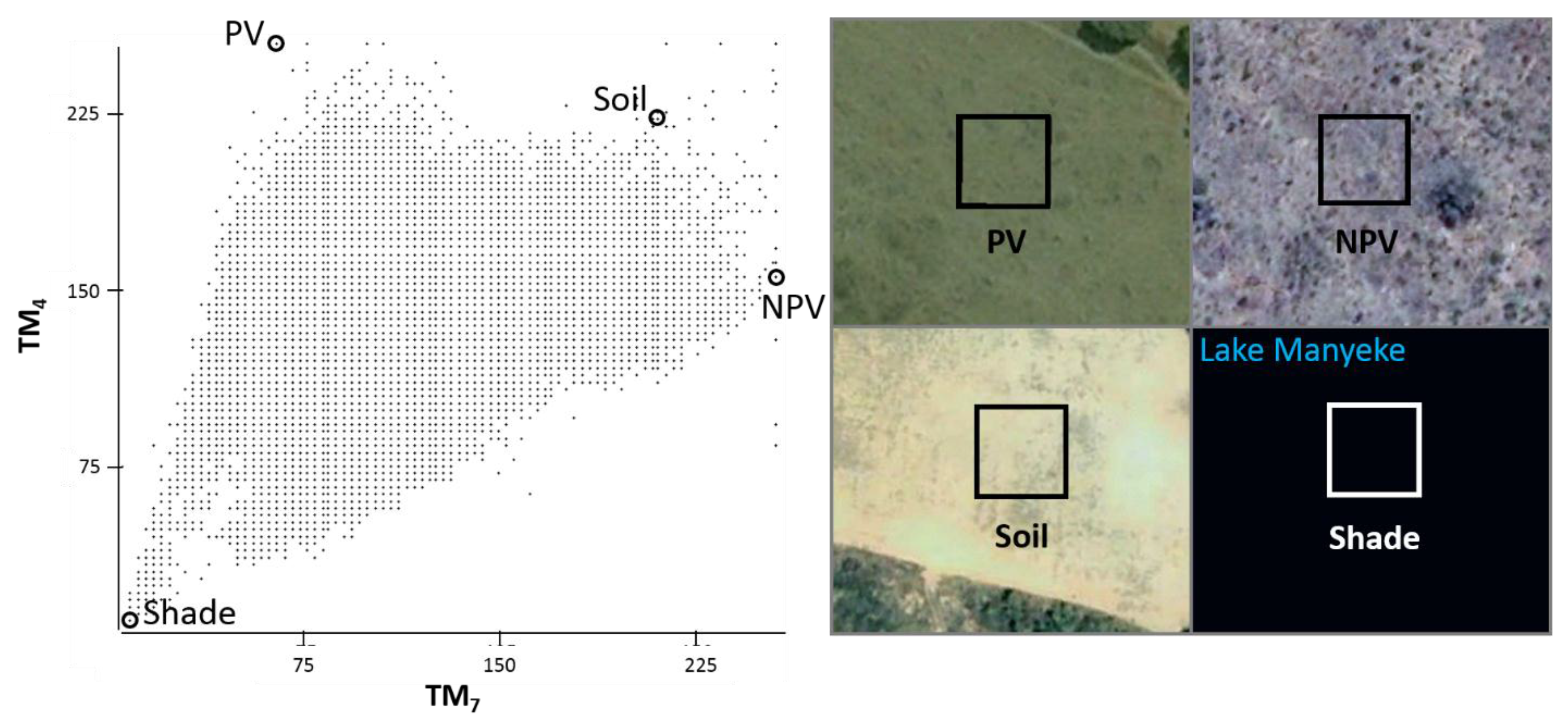A Sequential Maximum Angle Convex Cone (SMACC) [69], utilizing a residual minimization model, was used to identify a pseudo set of image endmembers that were displayed in a scatterplot amongst all pixels in the TM image as reference locations that would guide endmember selection. The set of four endmembers used in this analysis was selected through iterative testing of candidate pixels at reference locations, representing photosynthetic vegetation (PV), soil, non-photosynthetic vegetation (NPV), and shade components (Figure 4). Results of the constrained model showed few pixels with values below 0 or above 1 and a mean RMS error of 5.538 indicating that the selected endmembers effectively characterized the landscape. An inspection of RMS distribution revealed the highest error pixels concentrated in areas that seasonally inundate with water, however the magnitude of error was not considered serious enough to warrant modification of the model. The library of candidate predictors utilized in the logit model consisted of six difference variables (one for each band pair, 1–5, and 7) and four fraction images. Predictor values were extracted at the sampled locations and collated (Operation 8, Figure 2).

Figure 4. (Left): Location of selected endmembers in scatterplot where Landsat TM band 4 is assigned to the y-axis and band 7, the x-axis. Values of X and Y-Axes are at-surface reflectance. (Right): Endmember pixel boundaries mapped and overlaid on high-resolution imagery (Google Earth).

Figure 4. (Left): Location of selected endmembers in scatterplot where Landsat TM band 4 is assigned to the y-axis and band 7, the x-axis. Values of X and Y-Axes are at-surface reflectance. (Right): Endmember pixel boundaries mapped and overlaid on high-resolution imagery (Google Earth).

The type of error that we detect within subgroups is always commission error. Our logit models are used to identify misclassified pixels of the commissioned category, assigning a value of 1 to cases associated with the latter category and 0 to cases associated with the primary category to which the subgroup has membership. For example, we wanted to identify misclassified savanna within the cropland_3 subgroup, correcting the commissioning of savanna by cropland, so an outcome value of 1 was assigned to savanna cases and outcome value of 0 to cropland. The 10 candidate predictors were input to the logit model using backward stepwise selection (Operation 9, Figure 2). The significance level for removal was set at 0.10 and classification cutoff at 0.5. Overall fit of the model was evaluated using scalar measures of fit, such as log-likelihood, as well as information based measures (70). The likelihood ratio test (G²) compares the log likelihoods of the full and constrained model (i.e., a model with all coefficients but the intercept constrained to zero), and is reported as a chi-square statistic, with degrees of freedom and a statistical significance level. The likelihood ratio test allowed us to test the hypothesis that all model coefficients except the intercept were zero. Common pseudo-R square measures, such as McKelvey and Zavoina’s R² and Nagelkerke R² were used to assess the adequacy of the model. We also used the Hosmer and Lemeshow's goodness-of-fit test to compare predicted to observed frequencies, whereby a test with a large p-value indicates a good fit between the model and the data. Finally, to compare full (non-nested) to nested models we employ information measures of fit. Comparisons were made between the full, or non-nested (10 predictor), and nested (4 predictor) models using the difference in the Bayesian Information Criterion (BIC) measures for the two models (where an absolute difference of 2–6 suggests positive evidence, 6–10 indicates strong evidence, and a difference greater than 10 suggests very strong evidence in favor of the nested model [70]. Using Erdas IMAGINE’s Model Builder, parameters returned from the nested logit model were applied to the predictor layers, utilizing the subgroup thematic map to restrict the operation to the spatial extent of the strata of interest (Operation 10, Figure 2). Pixels within the subgroup were recoded to the appropriate land cover based on a threshold probability of 50% (Operation 11, Figure 2). Operations 5, 8–11 (Figure 2) were repeated for the remainder of high error subgroups. Once all high error subgroups were addressed, validation was performed using the dataset generated in (Operation 3, Figure 2).

3. Results

The first stage supervised classification yielded an overall accuracy for five primary land covers of 80.10%. The greatest error was observed within the savanna class where omission error was nearly 42%. Likewise, high commission error was found in the cropland and settlement categories at 24% and 28% respectively. Primary category subgroups identified as having high error were subsequently reclassified. Model parameters and statistics evaluating model fit are provided from two subgroup reclassifications: cropland_3 (Model 1) and settlement_2 (Model 2).

3.1. Evaluation of Model 1: Cropland_3 Subgroup

Four predictors were selected in the cropland_3 subgroup model to differentiate misclassified savanna from cropland: Fraction_veg, Fraction_Soil, Fraction_Litter, and the seasonal difference in near-infrared reflectance (Difference_B4). The likelihood ratio test, evaluating the four predictors as a group, was highly significant (G²162.65, df = 4, p < 0001). The Hosmer-Lemeshow goodness-of-fit (Χ²0.519, df = 8, sig. = 1.000) as well as two pseudo R-square values (McKelvey and Zavoina R² = 0.803 and Nagelkerke R² = 0.803) provided further support for the model fit. A comparison of nested and non-nested models offered positive evidence in favor of the nested (4 predictor) model over the full (10 predictor) model (difference in BIC = 3.816). All predictors contributed significantly to the model at a significance level of 0.001. A one unit increase in the difference of near-infrared reflectance increased the log odds of a pixel being savanna by 0.06, whereas the soil, vegetation, and litter fractions all decreased the log odds of a pixel being savanna, in order of decreasing magnitude (Table 3a).

Of the 80 known savanna plots within the cropland_3 thematic category, 74 were classified correctly, and 89 of the known 96 cropland plots classified correctly for an overall accuracy of 92.6% (Table 3b). Positive and negative predictive values (PPV and NPV) were calculated (%) with accompanying confidence intervals (Equation A1). PPV and NPV values indicated high probability of a plot being savanna when the test is positive, and high probability of a plot being non-savanna when the test is negative. Recoding pixels with p ≥ 0.5 reduced the spatial extent of the cropland_3 thematic category by 53.15%, from roughly 294 thousand hectares to 156 thousand while, simultaneously, reducing commission error of cropland and omission error of savanna.

Table 3. (a) Summary of predictor effects for cropland_3 subgroup model. (b) Classification table for cropland_3 subgroup model. Classification cutoff value is 0.500. PPV = Positive predicted value and NPV = Negative predicted value.

(a)
Predictor	β	SE β	eβ	Wald’s χ2 (df = 1)
FractionVeg	−0.2089***	0.0423	0.8115	24.36***
FractionSoil	−0.4225***	0.0985	0.6554	18.38***
FractionLitter	−0.1428***	0.0502	0.869	8.10***
DifferenceB4	0.0604***	0.0130	1.0622	21.57***
Constant	12.2058***	2.2976	NA	NA
(b)
Observed		Predicted
		Land Cover		Percentage Correct
		Cropland	Savanna
Land cover Cropland		89	7	92.7
Savanna		6	74	92.5
Overall Percentage				92.6
PPV: 91.36%; 95% CI: 82.99% – 96.44%
NPV: 93.68%; 95% CI: 86.75% – 97.63%

***p < 0.001.

Table 3. (a) Summary of predictor effects for cropland_3 subgroup model. (b) Classification table for cropland_3 subgroup model. Classification cutoff value is 0.500. PPV = Positive predicted value and NPV = Negative predicted value.

(a)
Predictor	β	SE β	eβ	Wald’s χ2 (df = 1)
FractionVeg	−0.2089***	0.0423	0.8115	24.36***
FractionSoil	−0.4225***	0.0985	0.6554	18.38***
FractionLitter	−0.1428***	0.0502	0.869	8.10***
DifferenceB4	0.0604***	0.0130	1.0622	21.57***
Constant	12.2058***	2.2976	NA	NA
(b)
Observed		Predicted
		Land Cover		Percentage Correct
		Cropland	Savanna
Land cover Cropland		89	7	92.7
Savanna		6	74	92.5
Overall Percentage				92.6
PPV: 91.36%; 95% CI: 82.99% – 96.44%
NPV: 93.68%; 95% CI: 86.75% – 97.63%

***p < 0.001.

3.2. Evaluation of Model 2: Settlement_2 Subgroup

Four predictors were selected for the settlement_2subgroup model to differentiate cropland from settlement: Fraction_veg, Fraction_Litter, Fraction_Shade, and the seasonal difference in visible green reflectance (Difference_B2). The likelihood ratio test was statistically significant (G²54.31, df = 4, p < 0.0001). The Hosmer-Lemeshow test (Χ² 7.736, df = 8, sig. = 0.460) and pseudo R² values indicated a good model fit, (McKelvey and Zavoina R² = 0.798 and Nagelkerke R² = 0.697). A comparison of nested and non-nested models (4 predictor vs. 10 predictor model) strongly favored the nested over the full model (difference in BIC = 15.729). All predictors were statistically significant at the 0.01 level of significance. A one unit change in Fraction_Litter resulted in the greatest increase in log odds of a pixel being cropland, followed by the vegetation and shade fractions. Seasonal difference in visible green lowered the log odds of a pixel being cropland. (

Table A2. Summary of predictor effects for Settlement_2 subgroup model.

Predictor	β	SE β	eβ	Wald’s χ2 (df = 1)
FractionVeg	0.4408**	0.1474	1.5539	8.94**
FractionLitter	0.5288**	0.1840	1.6968	8.25**
FractionShade	0.4259**	0.1548	1.5310	7.57**
DifferenceB2	−0.2802***	0.0773	0.7556	13.14***
Constant	−33.6832**	12.7889	NA	NA

**p < 0.01; ***p < 0.001

).

Of the 52 known cropland plots, 48 were classified correctly, and 18 of the known 26 non-cropland plots classified correctly for an overall accuracy of 84.6% (

Table A3. Classification table for settlement_2 subgroup model. Classification cutoff value is 0.500. PPV = Positive predicted value and NPV = Negative predicted value.

Observed	Predicted
	Land Cover		Percentage Correct
	Settlement	Cropland
Land cover Settlement	18	8	69.2
Cropland	4	48	92.3
Overall Percentage			84.6
PPV: 85.71%; 95% CI: 73.77% – 93.61%
NPV: 81.82%; 95% CI: 59.7% – 94.70%

). Omission error of cropland decreased and commission error of settlement was no longer detected. PPV and NPV both exceeded 82%, however, confidence intervals were much broader than those observed in the previous model. Recoding reduced the size of the settlement_2 thematic category by 33.3%, removing all error detected by the validation dataset.

A comparative assessment between the initial classification and post-correction classification revealed an absolute reduction in cropland commission error of 17.24% to an error of 7.04%, and decrease in omission error of 3.4% to 13.16% (Table 4). The greatest reduction in error was found in the savanna class where omission error was reduced by 28.78% although this resulted in a slight uptick in commission error of 3.08%. Overall, no measure of error in any category exceeded 15%.

Table 4. Error assessment of thematic land cover map at Path: 172 and Row: 071. Absolute changes in errors of omission and commission are reported in the last two columns. These values reflect the impact of error correction measures.

Class	Reference Total	Classified Total	No. Correct	εOmission	εCommission	Abs. Change εOmission	Abs. Change εCommission
Forest	108	116	104	3.70	10.34	−1.86	−10.59
Cropland	152	142	132	13.16	7.04	−3.40	−17.24
Savanna	152	155	132	13.16	14.84	−28.78	3.08
Settlement	40	40	40	0.00	0.00	0.00	−28.57
Water	25	24	24	4.00	0.00	4	0.00
Total	477	477	432
Overall Accuracy: 90.57

Table 4. Error assessment of thematic land cover map at Path: 172 and Row: 071. Absolute changes in errors of omission and commission are reported in the last two columns. These values reflect the impact of error correction measures.

Class	Reference Total	Classified Total	No. Correct	εOmission	εCommission	Abs. Change εOmission	Abs. Change εCommission
Forest	108	116	104	3.70	10.34	−1.86	−10.59
Cropland	152	142	132	13.16	7.04	−3.40	−17.24
Savanna	152	155	132	13.16	14.84	−28.78	3.08
Settlement	40	40	40	0.00	0.00	0.00	−28.57
Water	25	24	24	4.00	0.00	4	0.00
Total	477	477	432
Overall Accuracy: 90.57

Table 5. Error assessment of combined thematic maps from Path: 071 Row: 072, Path: 072 Row: 072, and Path: 073 Row: 071. Errors of omission and commission are reported in the body of the table, overall accuracy at the bottom.

Class	Reference Total	Classified Total	No. Correct	εOmission	εCommission
Forest	288	298	265	7.99	11.07
Cropland	421	410	370	12.11	9.76
Savanna	349	374	302	13.47	19.25
Settlement	100	80	78	22.00	2.50
Water	86	82	82	4.65	0.00
Total	1244	1244	1097
Overall Accuracy: 88.18

Table 5. Error assessment of combined thematic maps from Path: 071 Row: 072, Path: 072 Row: 072, and Path: 073 Row: 071. Errors of omission and commission are reported in the body of the table, overall accuracy at the bottom.

Class	Reference Total	Classified Total	No. Correct	εOmission	εCommission
Forest	288	298	265	7.99	11.07
Cropland	421	410	370	12.11	9.76
Savanna	349	374	302	13.47	19.25
Settlement	100	80	78	22.00	2.50
Water	86	82	82	4.65	0.00
Total	1244	1244	1097
Overall Accuracy: 88.18

The method described in this paper was subsequently applied to the adjacent datasets, categorizing land cover within the TM footprints at Path: 172 Row: 072 and Path: 173 Row: 071 (Figure 5). In total, 4 primary category subgroups were reclassified within the former footprint and 6 subgroups within the latter. Overall classification accuracy in the Path: 172 Row: 072 footprint was 85.4% and 86.5% in Path: 173 Row: 071. Cropland omission error was 12.8% and 7.3% respectively, commission error 9.4% and 14.2% (

Table A4. Accuracy assessment of the southern adjacent classification at Path: 172 Row: 072 and western adjacent classification at Path: 071 Row: 073.

Path: 172 Row: 072
Class	Reference Total	Classified Total	No. Correct	εOmission	εCommission
Forest	71	73	68	14.23	6.85
Cropland	133	128	116	12.78	9.37
Savanna	102	117	93	8.82	10.51
Settlement	39	29	28	18.21	3.45
Water	31	29	29	6.45	0
376	376	375	334
Overall Accuracy: 88.83
Path: 173 Row: 071
Forest	109	110	105	3.67	4.55
Cropland	137	148	127	7.3	14.19
Savanna	94	95	83	11.70	12.63
Settlement	21	9	8	33.33	6.67
Water	30	29	29	3.33	0.00
Total	391	391	358
Overall Accuracy: 91.56

). Finally, classification error was assessed for the combined footprints. Overall accuracy was reported at 88.18% with 1097 out of 1244 locations of known land cover classified correctly (Table 5). Omission error within the primary cropland class was slightly higher than commission error but both reasonably low. Errors of commission were high for the savanna class at 19.25% however, almost 66% of the error is attributable to confusion with the forest class. Of the 72 non-savanna plots classified as savanna, 43 were forest and 23 cropland. The largest recorded error was found in the settlement class, the majority of which was attributable to settlement misclassified as cropland.

Figure 5. Thematic land cover map of combined scenes at Path: 172 Row: 071, Path: 172 Row: 072, and Path: 173 Row: 071. White areas were obscured by cloud.

Figure 5. Thematic land cover map of combined scenes at Path: 172 Row: 071, Path: 172 Row: 072, and Path: 173 Row: 071. White areas were obscured by cloud.

4. Discussion

Reliably mapping cropland within smallholder-dominated savannas is critical to determining total area under crop and the distribution of cropland on the African continent. The workflow, and application of techniques, outlined in this paper delineates cropland within the savanna landscape of Zambia. The potential future applications of the protocol presented here could support policy initiatives aimed at achieving food security and support the frequent monitoring of food security in the region, as well as improve our understanding how seasonal climate variability affects regional crop production.

The suite of complementary remote sensing techniques used in this analysis are familiar to remote sensing researchers. Our contribution lies in the integration of these techniques in a manner that capitalizes on the salient utility of each one. The data-driven unsupervised clustering algorithm (ISODATA) segments pixels into natural clusters that reflect the underlying spectral structure of the data [71]. Through random sampling of unsupervised clusters, we are able to capture variability within primary land cover categories that is representative of conditions throughout the study area in an unbiased training dataset. Likewise, clustering training data into primary category subgroups and parameterizing a MLC with subgroup spectra has two distinct advantages. First, thematic output is produced where commission error can be detected and isolated within strata of primary categories. Second, spectral variability is reduced within classes which minimizes the number of confused primary categories within subgroups and reduces spectral noise, helping prevent over-fitting of the logistic model. The targeted reclassification that we adopt in this approach accounts for large spectral variability that is typically characteristic of generic land cover categories. By reclassifying within subgroups of primary categories we are able to treat spectral confusion between identical pairs of primary land covers uniquely within different subgroups.

While our selection of model variables is consistent with previous research [21,22,23,42,43,44,45] we have reduced the temporal requirements in the model and combined phenological measures with sub-pixel fractions of pure surface components. With this approach, we are able to address spectro-temporal similarity that cannot be addressed with phenological variables alone. From a pool of ten candidate variables, logit models are utilized to largely correct commission error in select primary category subgroups affecting the accuracy of the cropland category. For example, commission error resulting from savanna misclassified as cropland was reduced by over 22% (absolute change) for the combined scenes; commission error resulting from cropland misclassified as settlement was reduced by almost 35% (absolute change) for the combined scenes. These correction measures drove errors of omission and commission within the overall cropland class down to 12% and 10%, respectively.

Although image data acquired during the rainy season could potentially enhance spectral separation between cropland and the surrounding land cover, cloud-free data was not available. We have, however, demonstrated that data acquired at time points bracketing the temporal window of the growing season can be used to accurately delineate cropland. Admittedly, separation between settlement and cropland is more challenging without an image acquired during the growing season. We were able to eliminate much of the detected commission error within high-error settlement subgroups but omission error remained rather high at 22%, but these areas constitute a fraction of 1 percent of the study area. Although the spatial extent of the error was rather small, alternative predictors need to be evaluated to better address the cropland-settlement confusion, particularly for study areas with a larger urban presence or higher density of villages.

There are no major limitations of this approach as far as data availability. Temporal data requirements are minimal and images acquired during the growing season are not requisite. Both recent and historical Landsat data is available through the USGS Global Visualization viewer (http://glovis.usgs.gov/), Earth Explorer (http://earthexplorer.usgs.gov/), and a number of other online sources. Continuity missions such as Landsat 8 Operational Land Imager (OLI), and the planned Sentinel-2 satellite constellation, will allow the methods to be extended and enhanced with improved instrumentation.

The logit models are rather unrestrictive with the primary requirements being independent data points and categorical outcomes. However, with the use of logit models, care should be taken to avoid over-fitting by using a minimal number of predictors with an adequate number of observations.

The method is heavily dependent on repetitive sampling that requires high-resolution imagery for land cover coding. The difficulty and expense of obtaining this imagery, particularly for Africa, makes Google Earth the most viable alternative currently. There are, however, other approaches being proposed, such as DIYlandcover/Mapping Africa [72,73]. In this approach, crowdsources generate land cover data and geometric details of fields. DIYlandcover has the potential to be coupled with computer algorithms adapted for land cover mapping, iteratively training the algorithm and identifying the areas of high error through each iteration. The method we propose in this paper could be usefully paired with a crowdsourcing platform such as this where active learning takes place and iterations continue until the desired accuracy is achieved.

5. Conclusions

The application of this workflow, with additional testing in other savanna range countries and semi-arid landscapes, provides a potentially valuable tool to assist and inform regional and national food security policies, the development of crop failure early warning systems, and natural resource management policies. While the emphasis in this analysis was on the delineation of cropland, pasture is another important component of agricultural activity in the Southern Province of Zambia, as well as in other savanna range countries on the continent. Pasture constitutes the main area for both commercial and small scale sector livestock production [74], and supports other savanna agroecosystems. Although pasture is often simply savanna in Africa, there are developed and managed pastures that are of interest. An avenue for further research is reliably identifying and discriminating pasture, as well as cropland, from savanna in order to provide a more comprehensive picture of the agricultural landscape.

References

1. World Bank. Fact Sheet: The World Bank and Agriculture in Africa. Available online: http://go.worldbank.org/GUJ8RVMRL0 (accessed on 15 September 2015).
2. New Partnership for Africa’s Development (NEPAD). Agriculture in Africa: Transformation and Outlook; New Partnership for Africa’s Development (NEPAD): Johannesburg, South Africa, 2013. [Google Scholar]
3. Brink, A.B.; Eva, H.D. Monitoring 25 years of land cover change dynamics in Africa: A sample based remote sensing approach. Appl. Geogr. 2009, 29, 501–512. [Google Scholar] [CrossRef]
4. Ramankutty, N.; Graumlich, L.; Achard, F.; Alves, D.; Chhabra, A.; DeFries, R.; Foley, J.; Geist, H.; Houghton, R.; Goldewijk, K.; et al. Global land-cover change: Recent progress, remaining challenges. In Land-Use and Land-Cover Change; Lambin, E., Geist, H., Eds.; Springer: Berlin, Germany, 2006; pp. 9–39. [Google Scholar]
5. United Nations; Department of Economic and Social Affairs, Population Division. World Population Prospects: The 2012 Revision, Highlights and Advance Tables; Working Paper No. ESA/P/WP.228; United Nations: New York, NY, USA, 2013. [Google Scholar]
6. Searchinger, T.D.; Estes, L.; Thornton, P.K.; Beringer, T.; Notenbaert, A.; Rubenstein, D.; Heimlich, R.; Licker, R.; Herrero, M. High carbon and biodiversity costs from converting Africa’s wet savannahs to cropland. Nature Clim. Change 2015, 5, 481–486. [Google Scholar] [CrossRef]
7. Morris, M.B.H.; Byerlee, D.; Savanti, P.; Staatz, J. Awakening Africa’s Sleeping Giant: Prospects for Commercial Agriculture in the Guinea Savannah Zone and Beyond; The World Bank: Washington, DC, USA, 2009. [Google Scholar]
8. Falkenmark, M.; Rockström, J. Building resilience to drought in desertification-prone savannas in sub-Saharan Africa: The water perspective. Nat. Resour. For. 2008, 32, 93–102. [Google Scholar] [CrossRef]
9. Verdin, J.; Funk, C.; Senay, G.; Choularton, R. Climate science and famine early warning. Philos. Trans. R. Soc. B: Biol. Sci. 2005, 360, 2155–2168. [Google Scholar] [CrossRef] [PubMed]
10. Fritz, S.; See, L.; You, L.; Justice, C.; Becker-Reshef, I.; Bydekerke, L.; Cumani, R.; Defourny, P.; Erb, K.; Foley, J.; et al. The need for improved maps of global cropland. EOS Trans. Am. Geophys. Union 2013, 94, 31–32. [Google Scholar] [CrossRef]
11. Garnett, T.; Appleby, M.; Balmford, A.; Bateman, I.; Benton, T.; Bloomer, P.; Burlingame, B.; Dawkins, M.; Dolan, L.; Fraser, D. Sustainable intensification in agriculture: Premises and policies. Science 2013, 341, 33–34. [Google Scholar] [CrossRef] [PubMed] [Green Version]
12. Fritz, S.; See, L.; McCallum, I.; Schill, C.; Obersteiner, M.; Van der Velde, M.; Boettcher, H.; Havlík, P.; Achard, F. Highlighting continued uncertainty in global land cover maps for the user community. Environ. Res. Lett. 2011, 6, 044005. [Google Scholar] [CrossRef]
13. Ramankutty, N.; Evan, A.T.; Monfreda, C.; Foley, J.A. Farming the planet: 1. Geographic distribution of global agricultural lands in the year 2000. Glob. Biogeochem. Cycles 2008, 22. [Google Scholar] [CrossRef]
14. Hannerz, F.; Lotsch, A. Assessment of Land Use and Cropland Inventories for Africa; Centre for Environmental Economics and Policy in Africa, University of Pretoria: Pretoria, South Africa, 2006. [Google Scholar]
15. Estes, L.; McRitchie, D.; Choi, J.; Debats, S.R.; Evans, T.; Guthe, W.; Ragazzo, G.; Zempleni, R.; Caylor, K. DIYlandcover: Crowdsourcing the Creation of Systematic, Accurate Landcover Maps. Available online: https://0-dx-doi-org.brum.beds.ac.uk/10.7287/peerj.preprints.1030v1 (accessed on 19 September 2015).
16. Leroux, L.; Jolivot, A.; Bégué, A.; Seen, D.L.; Zoungrana, B. How reliable is the MODIS land cover product for crop mapping sub-Saharan agricultural landscapes? Remote Sens. 2014, 6, 8541–8564. [Google Scholar] [CrossRef] [Green Version]
17. Hannerz, F.; Lotsch, A. Assessment of remotely sensed and statistical inventories of African agricultural fields. Int. J. Remote Sens. 2008, 29, 3787–3804. [Google Scholar] [CrossRef]
18. See, L.; Fritz, S.; You, L.; Ramankutty, N.; Herrero, M.; Justice, C.; Becker-Reshef, I.; Thornton, P.; Erb, K.; Gong, P. Improved global cropland data as an essential ingredient for food security. Glob. Food Secur. 2015, 4, 37–45. [Google Scholar] [CrossRef] [Green Version]
19. See, L.; Fritz, S.; Thornton, P.; Justice, C.; Becker-Reshef, I.; Leo, O.; Herrero, M.; You, L. Building a Consolidated Community Global Cropland Map. Available online: http://earthzine.org/2012/01/24/building-a-consolidated-community-global-cropland-map/ (accessed on 28 August 2015).
20. Millennium Ecosystem Assessment (MEA). Ecosystems and Human Well-Being; Island Press: Washington, DC, USA, 2005; Volume 5. [Google Scholar]
21. Müller, H.; Rufin, P.; Griffiths, P.; Barros Siqueira, A.J.; Hostert, P. Mining dense Landsat time series for separating cropland and pasture in a heterogeneous Brazilian savanna landscape. Remote Sens. Environ. 2015, 156, 490–499. [Google Scholar] [CrossRef]
22. Estes, A.B.; Kuemmerle, T.; Kushnir, H.; Radeloff, V.C.; Shugart, H.H. Land-Cover change and human population trends in the greater Serengeti ecosystem from 1984–2003. Biol. Conserv. 2012, 147, 255–263. [Google Scholar] [CrossRef]
23. Nutini, F.; Boschetti, M.; Brivio, P.A.; Bocchi, S.; Antoninetti, M. Land-Use and land-cover change detection in a semi-arid area of Niger using multi-temporal analysis of Landsat images. Int. J. Remote Sens. 2013, 34, 4769–4790. [Google Scholar] [CrossRef]
24. Jiang, Z.; Huete, A.R.; Chen, J.; Chen, Y.; Li, J.; Yan, G.; Zhang, X. Analysis of NDVI and scaled difference vegetation index retrievals of vegetation fraction. Remote Sens. Environ. 2006, 101, 366–378. [Google Scholar] [CrossRef]
25. Todd, S.W.; Hoffer, R.M. Responses of spectral indices to variations in vegetation cover and soil background. Photogramm. Eng. Remote Sens. 1998, 64, 915–922. [Google Scholar]
26. Huete, A.; Tucker, C. Investigation of soil influences in AVHRR red and near-infrared vegetation index imagery. Int. J. Remote Sens. 1991, 12, 1223–1242. [Google Scholar] [CrossRef]
27. Major, D.J.; Baret, F.; Guyot, G. A ratio vegetation index adjusted for soil brightness. Int. J. Remote Sens. 1990, 11, 727–740. [Google Scholar] [CrossRef]
28. Huete, A.R.; Jackson, R.D.; Post, D.F. Spectral response of a plant canopy with different soil backgrounds. Remote Sens. Environ. 1985, 17, 37–53. [Google Scholar] [CrossRef]
29. Duro, D.C.; Franklin, S.E.; Dubé, M.G. A comparison of pixel-based and object-based image analysis with selected machine learning algorithms for the classification of agricultural landscapes using SPOT-5 HRG imagery. Remote Sens. Environ. 2012, 118, 259–272. [Google Scholar] [CrossRef]
30. Gibbes, C.; Adhikari, S.; Rostant, L.; Southworth, J.; Qiu, Y. Application of object based classification and high resolution satellite imagery for savanna ecosystem analysis. Remote Sens. 2010, 2, 2748–2772. [Google Scholar] [CrossRef]
31. Lu, D.; Li, G.; Moran, E.; Freitas, C.C.; Dutra, L.; Sant’Anna, S.J.S. A comparison of maximum likelihood classifier and object-based method based on multiple sensor datasets for land-use/cover classification in the Brazilian Amazon. In Proceedings of 4th Geographic Object-Based Image Analysis (GEOBIA), Rio de Janeiro, Brazil, 7–9 May 2012; pp. 20–24.
32. Wessels, K.; van den Bergh, F.; Scholes, R. Limits to detectability of land degradation by trend analysis of vegetation index data. Remote Sens. Environ. 2012, 125, 10–22. [Google Scholar] [CrossRef]
33. Li, J.Y. The Research and Application of Methods Used in Grassland Sandy Desertification Monitoring Based on TM Data. Master’s Thesis, Chinese Academy of Agricultural Sciences, Beijing, China, 2011. [Google Scholar]
34. Dawelbait, M.; Morari, F. Limits and potentialities of studying dryland vegetation using the optical remote sensing. Ital. J. Agron. 2008, 3, 97–106. [Google Scholar] [CrossRef]
35. Camacho-De Coca, F.; García-Haro, F.J.; Gilabert, M.A.; Meliá, J. Vegetation cover seasonal changes assessment from TM imagery in a semi-arid landscape. Int. J. Remote Sens. 2004, 25, 3451–3476. [Google Scholar] [CrossRef]
36. Elmore, A.J.; Mustard, J.F.; Manning, S.J.; Lobell, D.B. Quantifying vegetation change in semiarid environments: Precision and accuracy of spectral mixture analysis and the normalized difference vegetation index. Remote Sens. Environ. 2000, 73, 87–102. [Google Scholar] [CrossRef]
37. Smith, M.O.; Ustin, S.L.; Adams, J.B.; Gillespie, A.R. Vegetation in deserts: I. A regional measure of abundance from multispectral images. Remote Sens. Environ. 1990, 31, 1–26. [Google Scholar] [CrossRef]
38. Gessner, U.; Machwitz, M.; Conrad, C.; Dech, S. Estimating the fractional cover of growth forms and bare surface in savannas. A multi-resolution approach based on regression tree ensembles. Remote Sens. Environ. 2013, 129, 90–102. [Google Scholar] [CrossRef] [Green Version]
39. Adams, J.; Smith, M.; Gillespie, A. In simple model for complex natural surfaces: A strategy for the hyperspectral era of remote sensing. In Proceedings of 1989 International Geoscience and Remote Sensing Symposium (IGARSS’89), Vancouver, BC, Canada, 10–14 July 1989.
40. Adams, J.B.; Sabol, D.E.; Kapos, V.; Almeida Filho, R.; Roberts, D.A.; Smith, M.O.; Gillespie, A.R. Classification of multispectral images based on fractions of endmembers: Application to land-cover change in the Brazilian Amazon. Remote Sens. Environ. 1995, 52, 137–154. [Google Scholar] [CrossRef]
41. Small, C. The Landsat ETM+ spectral mixing space. Remote Sens. Environ. 2004, 93, 1–17. [Google Scholar] [CrossRef]
42. Li, J.; Yang, X.; Jin, Y.; Yang, Z.; Huang, W.; Zhao, L.; Gao, T.; Yu, H.; Ma, H.; Qin, Z. Monitoring and analysis of grassland desertification dynamics using Landsat images in Ningxia, China. Remote Sens. Environ. 2013, 138, 19–26. [Google Scholar] [CrossRef]
43. Dawelbait, M.; Morari, F. Monitoring desertification in a savannah region in Sudan using Landsat images and spectral mixture analysis. J. Arid Environ. 2012, 80, 45–55. [Google Scholar] [CrossRef]
44. Brandt, J.S.; Townsend, P.A. Land use–land cover conversion, regeneration and degradation in the high elevation Bolivian Andes. Landsc. Ecol. 2006, 21, 607–623. [Google Scholar] [CrossRef]
45. Singh, N.; Glenn, N.F. Multitemporal spectral analysis for cheatgrass (Bromus tectorum) classification. Int. J. Remote Sens. 2009, 30, 3441–3462. [Google Scholar] [CrossRef]
46. Hogland, J.; Billor, N.; Anderson, N. Comparison of standard maximum likelihood classification and polytomous logistic regression used in remote sensing. Eur. J. Remote Sens. 2013, 46, 623–640. [Google Scholar] [CrossRef]
47. Dendoncker, N.; Rounsevell, M.; Bogaert, P. Spatial analysis and modeling of land use distributions in Belgium. Comput. Environ. Urban Syst. 2007, 31, 188–205. [Google Scholar] [CrossRef]
48. Gao, J.; Zhang, Y. Incorporating spectral data into logistic regression model to classify land cover: A case study in Mt. Qomolangma (Everest) national nature preserve. Int. J. Geogr. Inf. Sci. 2012, 26, 1845–1862. [Google Scholar] [CrossRef]
49. Dubovyk, O.; Menz, G.; Conrad, C.; Kan, E.; Machwitz, M.; Khamzina, A. Spatio-Temporal analyses of cropland degradation in the irrigated lowlands of Uzbekistan using remote-sensing and logistic regression modeling. Environ. Monit. Assess. 2013, 185, 4775–4790. [Google Scholar] [CrossRef] [PubMed]
50. Koutsias, N.; Karteris, M. Burned area mapping using logistic regression modeling of a single post-fire Landsat-5 thematic mapper image. Int. J. Remote Sens. 2000, 21, 673–687. [Google Scholar] [CrossRef]
51. USAID. USAID Zambia Country Development Cooperation Strategy 2011–2015. Available online: https://www.usaid.gov/sites/default/files/documents/1860/USAIDZambiaCDCS30Sept2011.pdf (accessed on 18 March 2015).
52. Rasmussen, P.E. Zambia 2015. Available online: http://www.africaneconomicoutlook.org/fileadmin/uploads/aeo/2015/CN_data/CN_Long_EN/Zambia_GB_2015.pdf (accessed on 18 March 2015).
53. United Nations Conference on Trade and Development (UNCTAD). An Investment Guide to Zambia: Opportunities and Conditions 2011; United Nations: Geneva, Switzerland, 2011. [Google Scholar]
54. Zambia Central Statistics Office. 2010 Census of Population and Housing. Available online: http://www.zamstats.gov.zm/report/Census/2010/National/2010%20Census%20of%20Population%20National%20Analytical%20Report.pdf (accessed on 18 March 2015).
55. Löw, F.; Duveiller, G. Defining the spatial resolution requirements for crop identification using optical remote sensing. Remote Sens. 2014, 6, 9034–9063. [Google Scholar] [CrossRef]
56. Markham, B.; Barker, J. Thematic mapper bandpass solar exoatmospheric irradiances. Int. J. Remote Sens. 1987, 8, 517–523. [Google Scholar] [CrossRef]
57. Chavez, P.S., Jr. Radiometric calibration of Landsat thematic mapper multispectral images. Photogramm. Eng. Remote Sens. 1989, 55, 1285–1294. [Google Scholar]
58. Teillet, P.; Fedosejevs, G. On the dark target approach to atmospheric correction of remotely sensed data. Can. J. Remote Sens. 1995, 21, 374–387. [Google Scholar] [CrossRef]
59. Kuemmerle, T.; Perzanowski, K.; Chaskovskyy, O.; Ostapowicz, K.; Halada, L.; Bashta, A.-T.; Kruhlov, I.; Hostert, P.; Waller, D.M.; Radeloff, V.C. European bison habitat in the Carpathian mountains. Biol. Conserv. 2010, 143, 908–916. [Google Scholar] [CrossRef]
60. Pekkarinen, A.; Reithmaier, L.; Strobl, P. Pan-European forest/non-forest mapping with Landsat ETM+ and CORINE land cover 2000 data. ISPRS J. Photogramm. Remote Sens. 2009, 64, 171–183. [Google Scholar] [CrossRef]
61. Velleman, P. Data Desk; Data Description, Inc.: New York, NY, USA, 1986. [Google Scholar]
62. Swain, P.H.; Davis, S.M. Remote sensing: The quantitative approach. IEEE Trans. Pattern Anal. Mach. Intell. 1981, 6, 713–714. [Google Scholar] [CrossRef]
63. Jensen, J.R. Thematic information extraction: Image classification. In Introductory Digital Image Processing: A Remote Sensing Perspective, 2nd ed.; Prentice Hall: Englewood Cliffs, NJ, USA, 1996; pp. 197–256. [Google Scholar]
64. Boles, S.H.; Xiao, X.; Liu, J.; Zhang, Q.; Munkhtuya, S.; Chen, S.; Ojima, D. Land cover characterization of temperate East Asia using multi-temporal vegetation sensor data. Remote Sens. Environ. 2004, 90, 477–489. [Google Scholar] [CrossRef]
65. De Colstoun, E.C.B.; Story, M.H.; Thompson, C.; Commisso, K.; Smith, T.G.; Irons, J.R. National park vegetation mapping using multitemporal Landsat 7 data and a decision tree classifier. Remote Sens. Environ. 2003, 85, 316–327. [Google Scholar] [CrossRef]
66. Oetter, D.R.; Cohen, W.B.; Berterretche, M.; Maiersperger, T.K.; Kennedy, R.E. Land cover mapping in an agricultural setting using multiseasonal thematic mapper data. Remote Sens. Environ. 2001, 76, 139–155. [Google Scholar] [CrossRef]
67. Hao, P.; Zhan, Y.; Wang, L.; Niu, Z.; Shakir, M. Feature selection of time series MODIS data for early crop classification using random forest: A case study in Kansas, USA. Remote Sens. 2015, 7, 5347–5369. [Google Scholar] [CrossRef]
68. Siachalou, S.; Mallinis, G.; Tsakiri-Strati, M. A hidden Markov models approach for crop classification: Linking crop phenology to time series of multi-sensor remote sensing data. Remote Sens. 2015, 7, 3633–3650. [Google Scholar] [CrossRef]
69. Gruninger, J.H.; Ratkowski, A.J.; Hoke, M.L. The sequential maximum angle convex cone (SMACC) endmember model. Proc. SPIE 2004, 5425. [Google Scholar] [CrossRef]
70. Long, J.S.; Freese, J. Regression Models for Categorical Dependent Variables Using Stata, Revised ed.; Stata Press: College Station, TX, USA, 2003. [Google Scholar]
71. Ball, G.H.; Hall, D.J. ISODATA, A Novel Method of Data Analysis and Pattern Classification. 1965. Available online: http://www.dtic.mil/cgi-bin/GetTRDoc?AD=AD0699616 (accessed on 15 September 2015).
72. Estes, L.; McRitchie, D.; Choi, J.; Debats, S.R.; Evans, T.; Guthe, W.; Luo, D.; Gagazzo, G.; Zempleni, R.; Caylor, K. Diylandcover: Crowdsourcing the creation of systematic, accurate landcover maps. PeerJPrePrints 2015, 3, e1266. [Google Scholar]
73. Debats, S.; Luo, D.; Estes, L.; Fuchs, T.J.; Caylor, K.K. A generalized computer vision approach to mapping crop fields in heterogeneous agricultural landscapes. PeerJPrePrints 2015, 3, e1688. [Google Scholar]
74. Aregheore, E.M. Country Pasture/Forage Resource Profiles; Island Press: Washington, DC, USA, 2009; Volume 5. [Google Scholar]