Article

Automatic Detection and Segmentation of Columns in As-Built Buildings from Point Clouds

1
Applied Geotechnologies Research Group, University of Vigo. Rúa Maxwell s/n, Campus Lagoas-Marcosende, Vigo 36310, Spain
2
Department of Cartographic and Land Engineering, Polytechnic School of Ávila, University of Salamanca, Calle de los Hornos Caleros, 50, Ávila 05003, Spain
*
Author to whom correspondence should be addressed.
Remote Sens. 2015, 7(11), 15651-15667; https://0-doi-org.brum.beds.ac.uk/10.3390/rs71115651
Submission received: 3 July 2015 / Accepted: 16 November 2015 / Published: 20 November 2015

Abstract

:
Over the past few years, there has been an increasing need for tools that automate the processing of as-built 3D laser scanner data. Given that a fast and active dimensional analysis of constructive components is essential for construction monitoring, this paper is particularly focused on the detection and segmentation of columns in building interiors from incomplete point clouds acquired with a Terrestrial Laser Scanner. The methodology addresses two types of columns: round cross-section and rectangular cross-section. Considering columns as vertical elements, the global strategy for segmentation involves the rasterization of a point cloud onto the XY plane and the implementation of a model-driven approach based on the Hough Transform. The methodology is tested in two real case studies, and experiments are carried out under different levels of data completeness. The results show the robustness of the methodology to the presence of clutter and partial occlusion, typical in building indoors, even though false positives can be obtained if other elements with the same shape and size as columns are present in the raster.

Graphical Abstract

1. Introduction

For more than two decades, 3D building reconstruction has become an active research topic in remote sensing, photogrammetry and computer vision communities [1,2,3]. This trend has continued due to the increasing demand of updated, accurate and automatically produced models [4]. Although several methodologies have been developed for the automatic reconstruction of a building interior and envelope based on point clouds and/or imagery, most of them are focused on reconstructing buildings that are already finished, whereas not much attention has been paid to buildings under construction.
A systematic dimensional and quality assessment of construction components during the early stage of the construction process is essential for the successful completion of a construction process within the time given, thereby saving costs. The direct costs of rework in the construction industry are approximately 5% of the total construction costs [5].
Currently, the methods for the dimensional analysis of construction components are mostly based on the use of remote-sensing instruments such as Total Stations. Although they are very accurate, their use is time consuming and subject to operator errors and are consequently impractical at a large scale [6]. Terrestrial Laser Scanners (TLS) have received increasing attention for the collection and analysis of three-dimensional data of the as-built status of large-scale civil infrastructures, either during the construction phase, the put into service phase or in the operation stage [7]. The geometric acquisition with TLS devices is fast, and point clouds have a relatively high quality in terms of accuracy, precision and resolution [8]. Prompt collection and analysis of data are essential for the active monitoring of the production during the construction phase of a project and for the automatic 3D layout of built assets. Within this context, production monitoring enables the comparison of the as-built state of a project with the as-designed state defined in the contractual agreement. The importance of production monitoring lies in its usability to provide the complete details of a facility and an updated layout, to track the changes based on decisions during construction, and to record the deviations from decisions, which are the limits of the technical characteristics of the acquisition device and registration errors if more than one scan position is needed [7].
Although Terrestrial Laser Scanners acquire accurate and productive geometric data, point clouds are composed of massive and raw information that should be processed to extract the information that is useful for the applications they are intended to serve. For example, a point cloud composed of several thousand partial 3D point clouds that describe a building in an early construction phase is not useful, although the geometric position of the constructed columns and beams, their cross-sections and/or their height are known, given that these are aspects of interest for construction monitoring. Therefore, there is an increasing need for the automatic processing of as-built 3D laser scanned data and more particularly the comparison of this as-built data to planned works. In recent years, intense efforts have been made to facilitate the automatic processing of 3D laser scanning data. Although most approaches aim at the reconstruction of as-built elements, quality control and monitoring require additional functionality [9]. For instance, in the field of quality control and monitoring, 3D laser scanners have been recently applied to the structural monitoring of dams [10]; to track Mechanical, Electrical, and Plumbing (MEP) components such as ducts, pipes and conduits [11]; to control slab flatness [12]; and to the performance of the dimensional quality assessment of precast concrete elements [13].
The focus of this work is to detect and segment both round cross-section and rectangular cross-section columns in buildings. Cylinder detection in point clouds has been extensively studied because of their importance and high presence in urban environments (i.e., light poles) or in industrial infrastructures (i.e., ducts, conduits, pipes).
Lari and Habib [14] provided a detailed review of cylindrical feature segmentation methods, classifying them into three categories: spatial-domain, parameter-domain and hybrid methods. The first category includes region-growing approaches, which are mostly based on the geometric properties of individual laser points through a Principal Component Analysis of the local neighborhood [15]. In spatial-domain methods, the quality of results is dependent on the quality of the initial values of the parameters and, consequently, dependent on the quality of data [14]. In this regard, the noise problem in region growing procedures has been recently addressed through the introduction of Robust Principal Component Analysis (RPCA) to calculate point normals [16], the use of statistical techniques for outlier detection and curvature estimation [17] or taking the maximum of the distribution of possible normals from an image created by filling the Hough transform accumulator [18], resulting in a reduction of over-segmentation present in other region growing procedures. Other features such as the density of projected points, point eigenvalues, and intensity have also been used to detect cylindrical vertical elements such as poles or trees in urban scenes [19,20,21]. These segmentation strategies involve the recovery of a local neighborhood for each 3D point and the extraction of different features followed by a classification process. Weinmann et al. [22] provided a recent review of these methods, mostly applied to urban scenes, in which data are acquired from a Mobile Laser Scanner, resulting in high-quality datasets in terms of data completeness.
In the parameter-domain category, methods are based on finding predefined parametric shapes. Parameters are initially estimated from the local neighborhood of each point, and detection is based on searching peaks in the attribute space. These methods are considered slow with regard to spatial-domain methods, especially if the number of parameters involved is high but are more robust to the presence of clutter and occlusions [23]. The Hough Transform is an approach belonging to this category. A cylinder is defined by five parameters, making the direct use of the Hough Transform impractical [24]. Alternatives to the direct use of the Hough Transform have been proposed in recent years to extract cylinders from point clouds. For example, pipes have been detected into orthogonal slices of point clouds using a 2D-based Hough Transform [25,26]. This methodology has also been used with regard to round cross-section column detection [27], although the methodology is tested under conditions of data completeness. Rabbani and van den Heuvel [24] introduced a sequential two-step Hough transform consistent on first detecting the direction of the cylinder axis (2D Hough Transform) and then obtaining the radius and pose (3D Hough Transform). Finally, the third category proposed by Lari and Habib [14] includes hybrid methods such as Random sample consensus (RANSAC), in which features are classified in the parameter domain and fitted in the spatial domain [28].
With regard to rectangular prism elements, most efforts have been focused on reconstructing only the visible planar surfaces from which they are compounded. For instance, indoor walls have been extensively recognized and modeled by surface-based methods [29,30,31,32], whereas only a few volumetric-based approaches have been developed [33,34]. Methods for fitting volumetric primitives to the data are more susceptible to inaccuracy and incompleteness of the data.
Whereas spatial-domain approaches directly extract features from data, parameter-domain approaches use previous knowledge to search for the most appropriate model. This fact makes parameter-domain approaches more robust in the presence of partial occlusion [23].
The main objective of this work is to develop a methodology to detect and segment both round and rectangular cross-section columns in buildings. Specific objectives of the paper are related to the robustness of the methodology under different levels of clutter, occlusion and data completeness typically present when building indoors. On the one hand, point cloud completeness depends on the scan positions from which data are acquired, which are determined according to the shape complexity and the occupied parts of the indoor building. On the other hand, indoor scenes are typically occluded and cluttered environments, during both the construction and use phases because of the presence of other objects such as auxiliary construction elements and furniture, respectively. The proposed methodology is based on model-driven techniques such as the Hough Transform and the Generalized Hough Transform. These techniques are robust in the presence of partial occlusion because they incorporate knowledge of the shape of the object to be recognized.
The paper is organized as follows. Section 2 describes the methodology developed for round cross-section and rectangular cross-section column reconstruction. Section 3 is focused on the results and the discussion extracted from the application of the methodology to two case studies under different levels of data completeness. Finally, Section 4 addresses the conclusions extracted from the work.

2. Methodology

This section presents the methodology proposed for the automatic detection and segmentation of 3D columns (Figure 1). Section 2.1 includes the preceding steps required for column detection, which is addressed in Section 2.2. Finally, Section 2.3 describes the segmentation of the column candidates in the point cloud.
Figure 1. Schema of the methodology proposed for column detection and segmentation.
Remotesensing 07 15651 g001

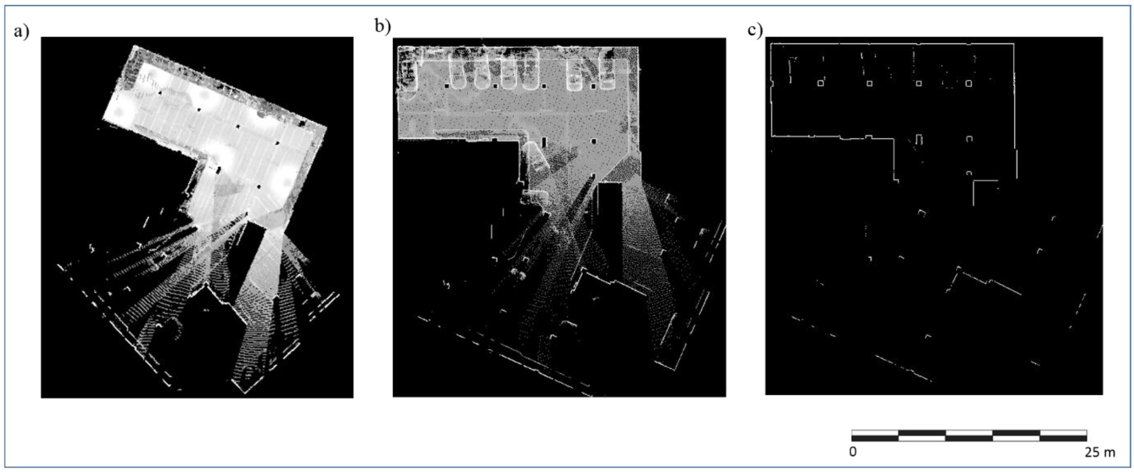
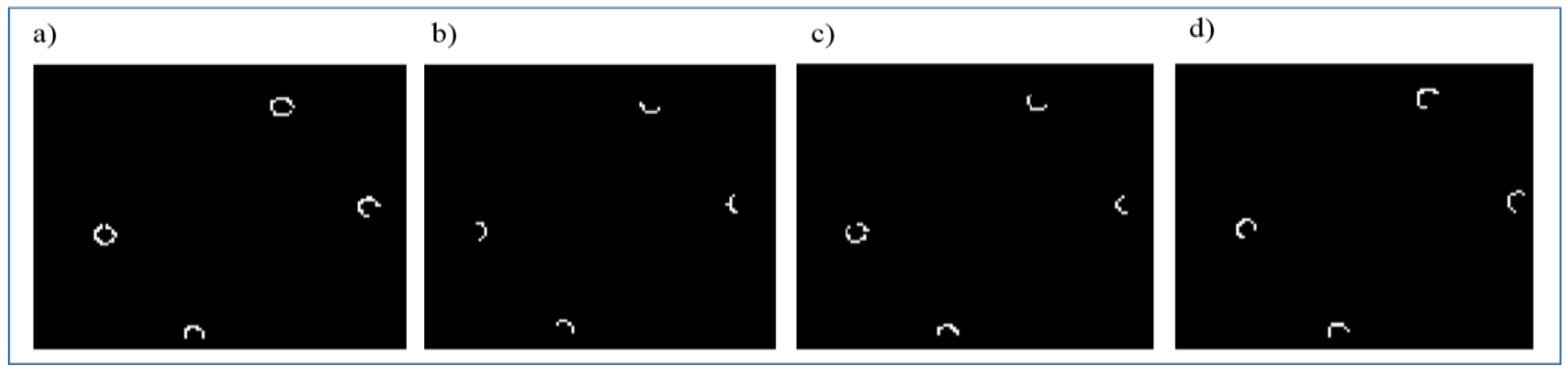
2.1. Building Rasterization

To fulfill the requirements of the subsequent steps, the point cloud with rectangular cross-section columns is rotated such that the building floor and/or ceiling are parallel to the XY plane and to walls. In this way, columns are ensured to be vertically oriented and column faces are parallel to the X-axis or Y-axis. The first condition is necessary for a correct rasterization, whereas the second is required by the column detection step, which is orientation dependent.
The rotation angles are estimated from the distribution of the normal vectors of the points, calculated using Principal Component Analysis. Normal vectors are clustered into three groups according to the X-, Y- and Z-axes using the k-means algorithm. Cluster centers are used to form a 3D rotation matrix from the aligned to the original coordinate system; inverse rotation is then applied [32].
Once the point clouds are oriented, they are converted to images, which are the inputs of column detection. The first step in building rasterization consists of the projection of the point cloud onto the XY plane. For this purpose, a rectangular matrix is created, and pixels are assigned with the number of points that fall inside each pixel (Figure 2). As a result, a gray-level raster is obtained by weighting values according to the minimum and maximum number of points. Columns are vertically oriented elements, so the pixels corresponding to these elements are expected to have a high value in the matrix [35].
Finally, raster images are submitted to a binarization to divide the image into two basic classes. The first class, with the value 1 (white), corresponds to the vertical elements such as walls or columns, with a high number of points in the corresponding pixels. The second class, with the value 0 (black) refers to the remaining indoor elements such as the ground or parked cars with a typical low number of points per pixel (Figure 2c). The binarization step requires the introduction of a threshold to convert the grayscale image (raster image) to a binary image. The threshold with a value in the range [0, 1] is relative to the signal levels possible for the image’s class and is automatically obtained following the Otsu method [36], which chooses the threshold that minimizes the intraclass variance of the black and white pixels.
Although edge pixels are the input to the subsequent column detection step, images are not submitted to an edge detection algorithm because column contours can already be considered edges.
Figure 2. Top view of a point cloud dataset (a), its correspondent raster after rotation (b), and the final binarized raster (c). Brightness and contrast are increased by 20% (b) and 40% (c) to improve its visualization.
Remotesensing 07 15651 g002

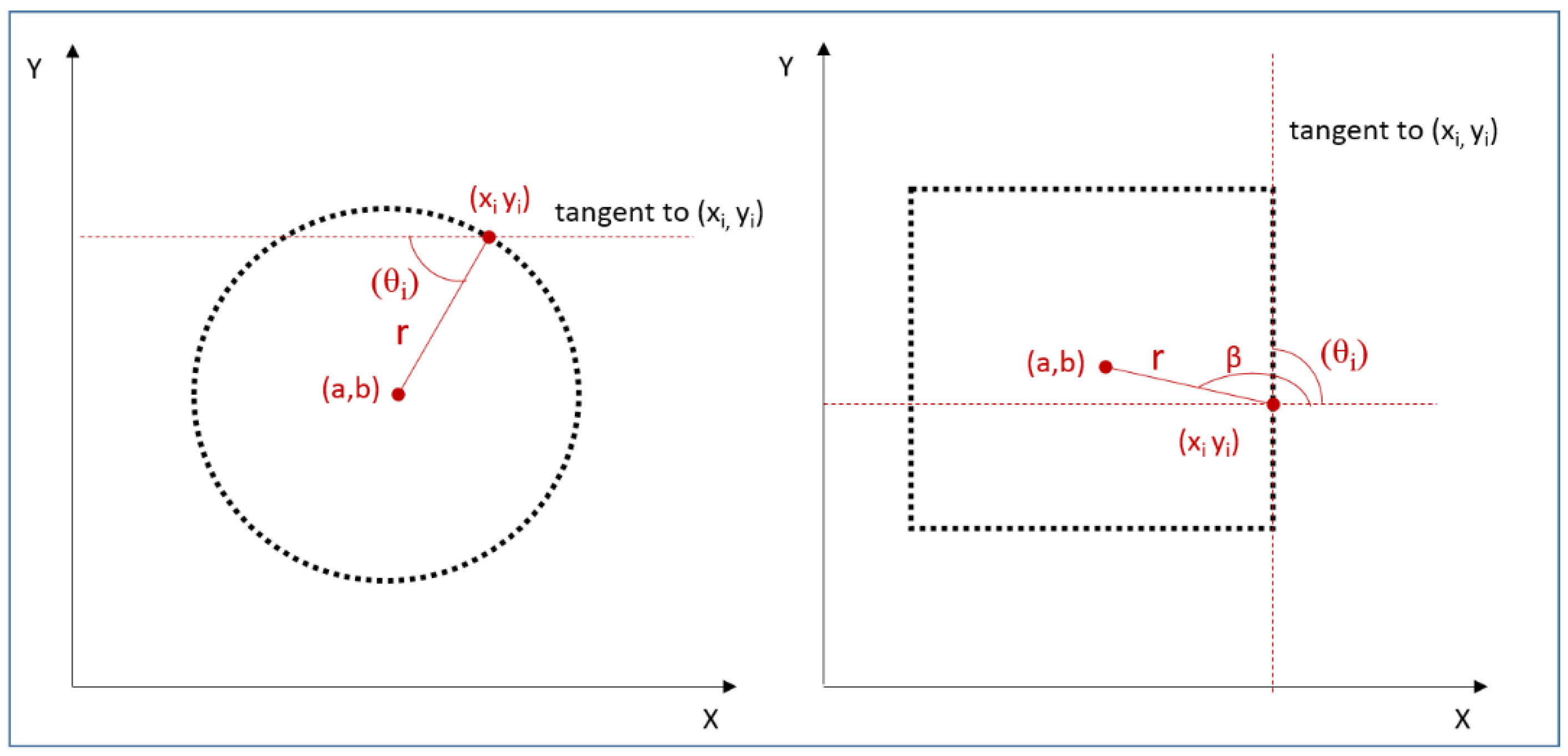
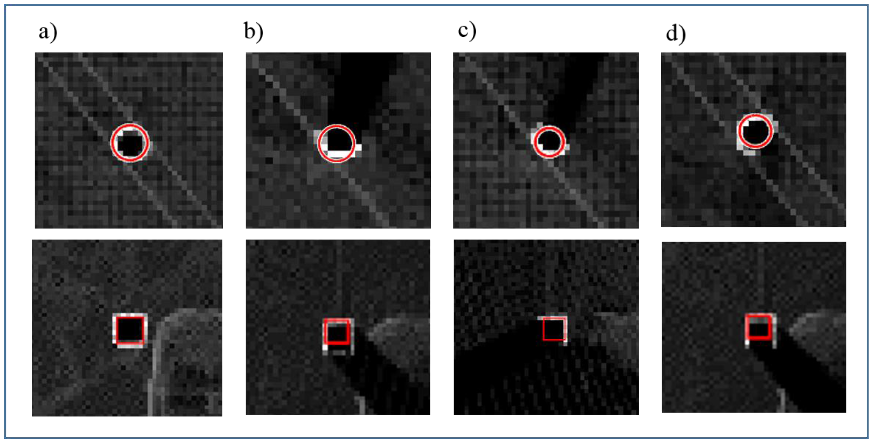
2.2. Column Detection

The detection of columns is based on the determination of parametric shapes, such as circles or rectangles, in an image. In this methodology, the use of the Circle Hough Transform is proposed to detect round columns in the image, whereas the Generalized Hough Transform is applied to the detection of rectangular columns.
Both techniques are based on the Hough Transform [37] developed for detecting objects, which can be defined with a few parameters such as lines, planes or circles. Although the Hough Transform is used to detect objects defined with a few parameters such as lines, planes or circles, the GHT [38] transforms the shape detection process into a maximum analysis problem so that arbitrary shapes can be detected [28].
Both techniques are used due to their robustness in the presence of noise, occlusion, varying illumination and invariance to scale changes [23]. The Circle Hough Transform (CHT) is implemented in Matlab© 2014 [39], whereas the Generalized Hough Transform (GHT) is self-implemented as in [32].
On the one hand, the Circle Hough Transform aims at finding circular shapes in an image. For a circle described as Equation (1), where (a,b) are the coordinates of the circle center and r is the radius, an arbitrary edge point (xi, yi) can be transformed into a right circular cone in the (a,b,r) parameter space.
(x − a)2 + (y − b)2 = r2
Each edge point contributes to a circle of radius r and is allowed to cast a vote in an output accumulator space. If all edge points lie on a circle, then the cones will intersect at a single point in (a,b,r) corresponding to the parameters of the circle. In this case, circle centers are estimated by detecting the peaks in the accumulator array. Whereas the classical CHT requires a 3-D array to store the votes for multiple radius searches, the implemented method uses a 2-D accumulator array (a,b) for which a previous radius estimation is needed: a radius range is specified as a two-element vector formed by a minimum radius and maximum radius. Furthermore, instead of edge pixels (xi,yi), edge orientation (θi) is used because it is computationally more effective (Figure 3, left).
Figure 3. Parameters involved in the CHT (left) and GHT (right) [9] for column detection.
Remotesensing 07 15651 g003
On the other hand, the GHT is implemented to find oriented rectangles, meaning that, if possible, rectangle sides should be parallel to the coordinate axis. The GHT uses a 4-D Accumulator Array (a, b, Sx, Sy), where a and b are the coordinates of the center point, and Sx and Sy are the scale parameters corresponding to width and length of the column, respectively. For each edge pixel, edge orientation is also calculated (θi) and used to find the corresponding vectors (r,β) in an R-table where the shape of a rectangle is stored and represented by its edge orientation (θi) and a vector defined (r,β) to an arbitrary center point (Figure 3, right). As in CHT, rectangles are estimated by searching for peaks in the 4-D accumulator array. To enforce the detection, minimum and maximum width and length are considered. Because the number of columns is unknown, a large number of columns are searched, resulting in over-detection. Finally, the most voted columns are selected as column candidates.
For each column shape, Figure 4 shows an example of a success and a failure in column detection.
Figure 4. Successful results in column detection (left) and failures (right) showed over the raster images. Brightness and contrast are increased by 40% to improve the visualization of the images.
Remotesensing 07 15651 g004

2.3. Column Segmentation and Parameterization

The 2D image parameters obtained from the previous step are transformed to the 3D coordinate system and used to segment the columns. The outcome of round cross-section detection consists of circle centers (x, y) in raster coordinates and radius. With regard to rectangular cross-sections, the results are the rectangle center (x, y) in raster coordinates and the height and width of the rectangle. Centers are transformed from the 2D raster coordinate system to the 3D point cloud coordinate system and radius, and height and width are used to define a circular and rectangular buffer, respectively. All points inside each buffer correspond to one column. In both cases, the buffer section is increased to ensure a complete segmentation of the column (Figure 5).
Figure 5. Image of two automatically segmented columns: round cross-section (left) and rectangular cross-section (right).
Remotesensing 07 15651 g005

3. Results and Discussion

This section addresses the results obtained from the application of the proposed methodology to different real case studies: a building foundation with round cross-section columns and an indoor garage with rectangular cross-section columns. In both cases, the approach has been tested under different levels of data completeness.

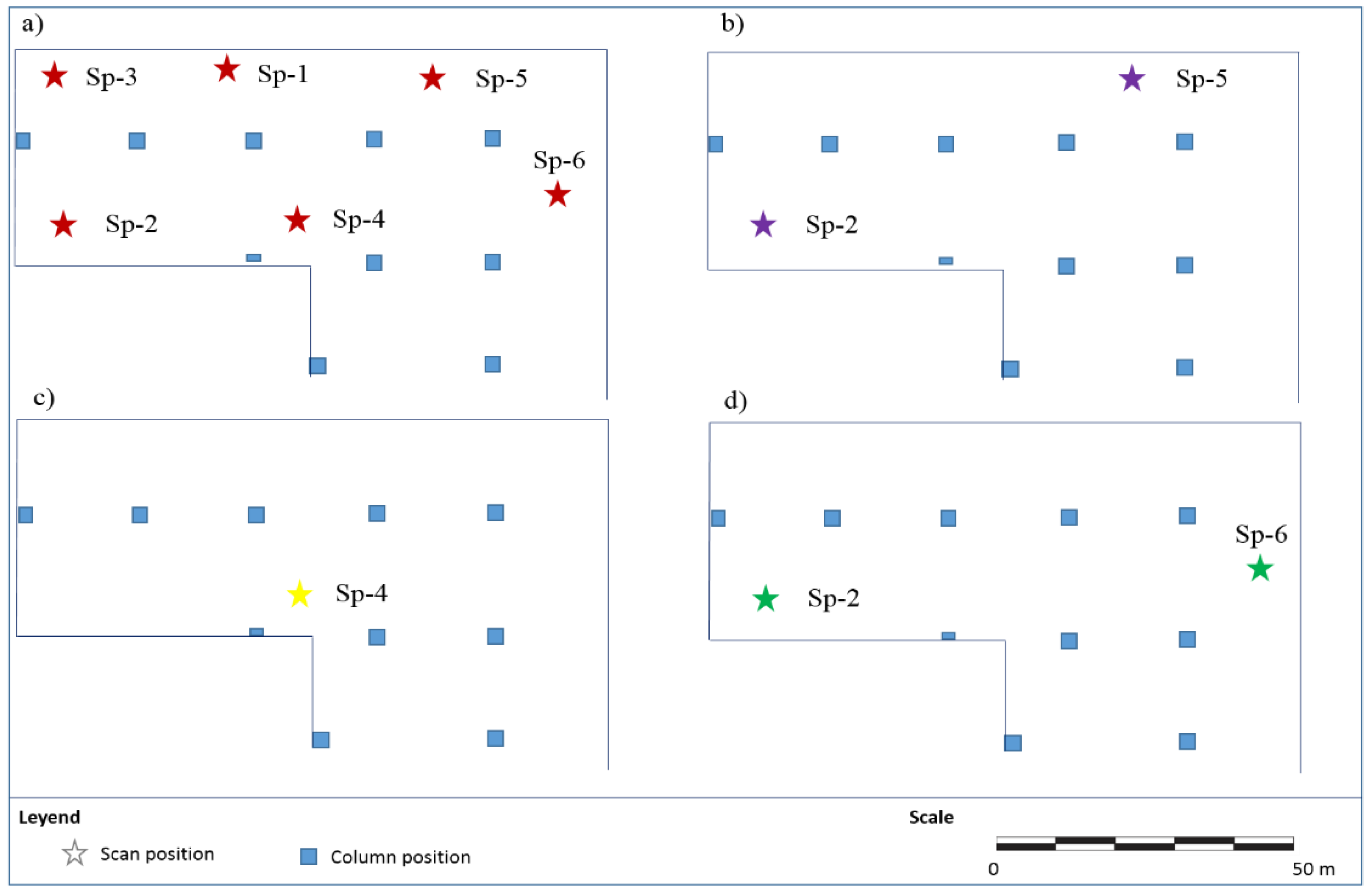
3.1. Data and Instruments

Datasets consist of point clouds obtained from a Terrestrial Laser Scanner, model FARO Focus 3D. The technical characteristics of the laser device are summarized in Table 1.
Table 1. Technical characteristics of the FARO Focus3D X 330 laser scanning device according to the manufacturer datasheet.
Technical Characteristics
Measurement range0.6 m to 330 m
Ranging error (25 m, one sigma)±2 mm
Step size (vertical/horizontal)0.009°/0.009°
Field of view (vertical/horizontal)300°/360°
Beam divergence0.011°
Measurement rate (points per second)122,000–976,000
Laser wavelength1550 nm
Two case studies are used for this work. On one side, a building foundation (case study 1) is chosen owing to the presence of visible columns with round cross-sections. On the other side, an indoor garage of a residential building (case study 2) is surveyed. Columns with rectangular cross-sections are present in the latter. Furthermore, several cars are parked in the garage, provoking occlusions. Figure 6 depicts an example of the point cloud of both case studies.
Figure 6. Example of the point cloud from the building foundation (left) and the indoor garage of a residential building (right).
Remotesensing 07 15651 g006
The geometry of a building interior is complex due to the high presence of objects that provoke occlusions, necessitating data acquisition from different positions to complete the acquisition of available information.
Once data are acquired, point clouds are registered into the same coordinate system. The origin of the coordinate system is settled in the origin of one of the laser scanner positions, and the remaining scan positions are registered by manually selecting at least four control points between them and the point cloud of reference. Registration is carried out by finding corresponding tie point pairs in two different range data. This process allows the coarse determination of the transformation parameters (rotation and translation), which minimize the sum of squared distances (SSD) among all point pairs. Afterwards, a fine registration is performed based on the ICP method [40]. For this work, registration is performed until error is inferior to 0.02 m. The first point cloud is submitted to a cleaning process to deselect the information corresponding to the exterior of the building (Figure 1, left). Both point clouds are filtered using a 0.05 m octree (for X, Y, and Z directions) to ensure uniform density because binarization is sensitive to high density variations [41]. The process is carried out using Riscan Pro software.
Figure 7 and Figure 8 show a schema of the experiment design. In both cases, the most complete dataset corresponds to experiment (a). Experiment (b) considers two scan positions placed at different sides of the building, whereas experiment (d) uses data from two scan positions located at the same side. Finally, one isolated scan position is considered for experiment (c).
Figure 7. A schema of the datasets considered in the indoor garage case study for testing the methodology under different levels of data completeness: complete dataset (a), two scan positions placed at different sides of the building (b), one isolated scan position (c), and two scan positions placed at the same side of the building (d).
Remotesensing 07 15651 g007

3.2. Building Rasterization
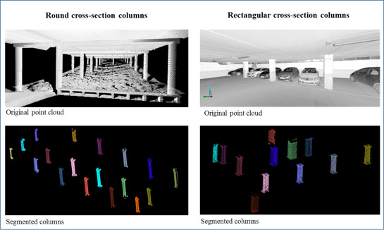
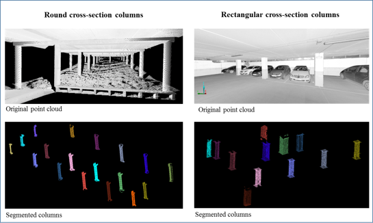
Building datasets are filtered using a 0.05 m octree and rasterized to the XY plane. The main results of this process are shown in Table 2. A coarse resolution of 0.08 m is selected, which is sufficient for column detection. Each case study has a different point cloud size and image size because they are formed by the combination of different scan positions.
Figure 8. The proposed methodology is tested through four tests depending on the data completeness for the round column case study: complete dataset (a), two scan positions placed at different sides of the building (b), one isolated scan position (c), and two scan positions placed at the same side of the building (d).
Remotesensing 07 15651 g008
Table 2. The results of the rasterization process.
Round Cross-section
Case Study 1.aCase Study 1.b.Case Study 1.cCase Study 1.d
Point cloud size (points)790,527380,995252,067454,849
Raster resolution (m)0.080.080.080.08
Image size (pixels)603 × 707557 × 594511 × 544572 × 707
Rectangular cross-section
Case study 2.aCase study 2.b.Case study 2.cCase study 2.d
Point cloud size (points)488,333247,832211,011288,571
Raster resolution (m)0.080.080.080.08
Image size (pixels)494 × 461484 × 430536 × 379447 × 398
After rasterization, raster images are submitted to binarization, whose threshold is calculated using the Otsu method [36]. Figure 9 shows the binarized images for the four experiments of the round cross-section case study. A centered area of the case study is selected to highlight the completeness of the information available. Figure 9a corresponds to the most complete dataset where central columns are acquired from different points of view and thus are completely depicted in the resulting image. Conversely, Figure 9c shows the result for the less complete dataset in which central pillars are partially depicted in the resulting image.
Figure 9. The same binarized area is shown for the experiments (a), (b), (c) and (d) (Figure 8) of the round cross-section case study.
Remotesensing 07 15651 g009

3.3. Column Detection

Binarized images are submitted to the column detection approach: circular columns are detected with CHT, and rectangular images are detected with GHT. In both cases, the approach is tested under different levels of point cloud completeness. Figure 10 shows that column detection operates under different levels of data completeness. Images on the top correspond to the same column of the round cross-section case study, whereas images on the bottom do the same with a column of the rectangular cross-section case study. The images on the left (case study 1.a and 2.a) correspond to detection when data are complete, whereas images b, c and d present the same column successfully detected under different levels of data completeness.
Figure 10. For each case study per column, an example of a column successfully detected with independence of data completeness. The results are shown over the raster image for experiments (a), (b), (c) and (d).
Remotesensing 07 15651 g010
The detection of rectangular columns is enforced with a minimum and maximum column size, 40 cm and 100 cm, respectively. Furthermore, given that the number of columns is not known, 50 bins are searched resulting in over-detection. Final candidates are selected based on their voting rate in such a way that columns with a voting rate superior to the 75th percentile are considered column candidates (first quartile).
To analyze the results, precision, recall and F1 score are evaluated. These parameters are based on the number of true positives (number of columns correctly labeled), the number of false positives (number of column candidates incorrectly labeled) and the number of true negatives (number of columns not detected). Precision, also called positive predictive value, represents the correctness of column detection such that true positives are evaluated with regard to total true and false positives. Recall, also known as sensitivity, indicates the ability to detect columns correctly; consequently, true positives are compared to existent columns. The F1 score combines recall and precision with equal weights to measure the accuracy of the method [42].
The results are shown in Table 3. Regarding recall, although 12/19 round cross-section columns and 7/10 rectangular cross-section columns were detected in all tests carried out (Section 3.1), the methodology is slightly dependent on the completeness rate. Undetected columns correspond to zones in the case studies where columns are not sufficiently acquired. Accordingly, case study 1.c and case study 2.c, acquired from one isolated scan position (Figure 7 and Figure 8, respectively), present lower rates of recall than those experiments acquired from different scan positions.
With respect to precision, case study 1 does not present false positives. These high rates of precision are obtained because of the absence of other objects in the image that could be confused in shape and size with columns. In case study 2, the presence of other elements in the image such as wall corners causes the presence of false positives, and therefore, its precision is lower (Figure 11).
Within the proposed methodology, the primary computational effort is concentrated on the column detection approach. With the purpose of quantifying computational effort, both CHT and GHT methods have been evaluated for different raster resolutions, considering an area of 200 m2 in plane XY for both case studies. Area is selected from a rectangle with dimensions of 10 × 20 m2 centered on the coordinate origin of the point cloud.
Table 3. Recall, precision and F1 scores for the case studies.
Round Cross-section
Case Study 1.aCase Study 1.bCase Study 1.cCase Study 1.d
Recall0.950.680.630.89
Precision1111
F1 score0.970.810.770.94
Rectangular cross-section
Case study 2.aCase study 2.bCase study 2.cCase study 2.d
Recall0.90.90.70.8
Precision0.690.640.530.67
F1 score0.780.750.610.72
Figure 11. Wall corners can be detected as rectangular cross-section columns being false positives. The results are shown over the raster image.
Remotesensing 07 15651 g011
The data have been processed on a computer with an Intel Core i7 processor with a 2.30 GHz processor frequency and 8 GB of RAM. Figure 12 shows the results of CPU time versus resolution for both methods. Although the Hough transform-based methods are considered slow, especially if the number of parameters of the transformation is larger, in this case, results on the order of 0.03 s and 1.89 s are obtained for processing an area of 200 m2 with a resolution of 0.08 m, for round (three parameters) and rectangular (four parameters) cross-sections, respectively. Short processing times are due to preprocessing steps, which minimize pixels subjected to the column detection approach (Figure 2).
Figure 12. Computational effort is evaluated for different resolutions considering an area of 200 m2: round cross-section method (left), rectangular cross-section method (right).
Remotesensing 07 15651 g012

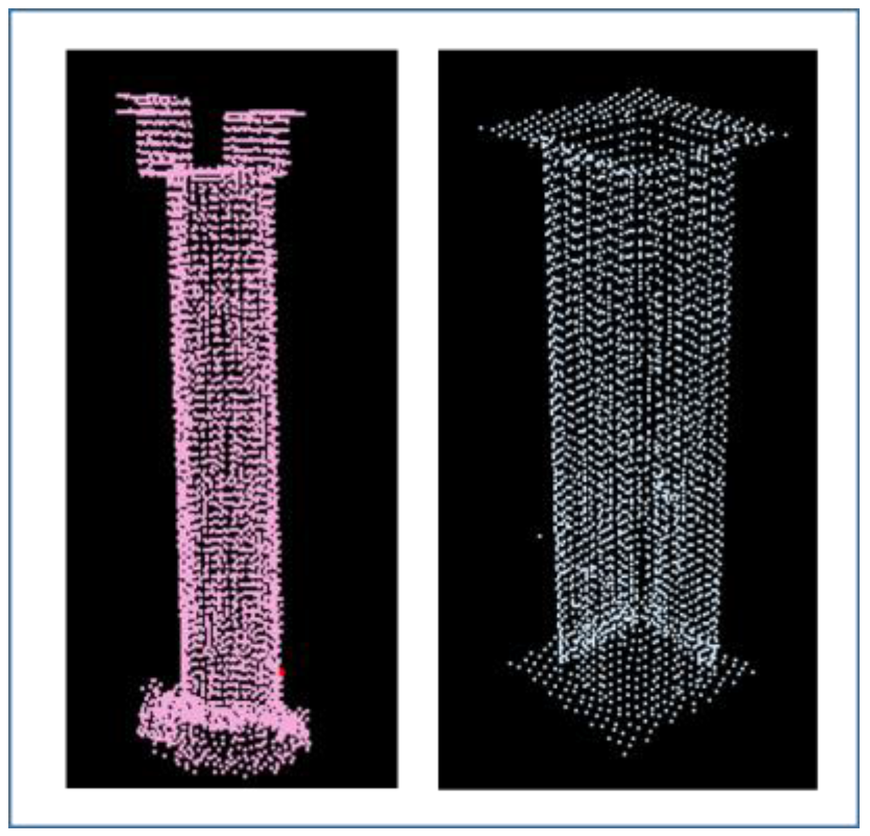
3.4. Column Segmentation

Finally, columns are segmented from the point cloud by creating a buffer from the parameters obtained in the previous section: center and radius for the round cross-section case study and center, width and height for the rectangular cross-section case study (Figure 13). The buffer is created by incrementing by 0.08 m (1 pixel size in this case) the parameters to ensure complete segmentation.
Figure 13. Image with segmented columns visualized with different colors (case study 1.a and case study 2.a).
Remotesensing 07 15651 g013

4. Conclusions

This paper presents a methodology for the detection and segmentation of columns in building interiors from point cloud data.
From the results, the following main conclusions can be drawn:
  • The proposed methodology is robust for column detection without submitting data to manual cleaning, therefore minimizing the processing time.
  • The detection step operates under different levels of data completeness. Therefore, it is robust to partial occlusions and clutter, which are very frequent in indoor environments.
  • False positives are obtained, especially if other elements with the same shape and size as columns are present in the XY raster. In the case of rectangular cross-section, false positives such as wall corners, information from other elements of the scene such as walls could be used for their identification as false positives.
  • The robustness of the methodology makes the acquisition of data from a complete point of view unnecessary and thus minimizes acquisition time.
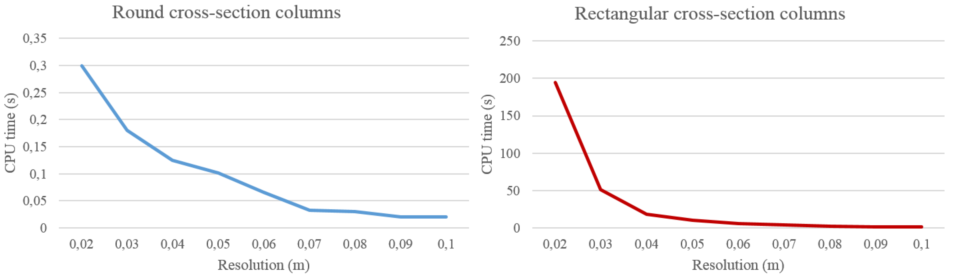
  • A coarse resolution in the rasterization process is enough for column detection.
In summary, incomplete point clouds enable the automatic detection and segmentation of columns in building interiors. A coarse rasterization is sufficient for detecting columns. The methodology could also be used in the geometrical characterization of section columns, but a finer resolution would be required. Base and top height could be determined from the height histograms of the segmented columns. Future work will address the quantitative analysis of data completeness for accurate detection and geometrical characterization of columns.

Acknowledgments

The authors thank Martin Bueno and Higinio González for acquiring data and the Ministerio de Economía y Competitividad (Gobierno de España) for the financial support given through a human resources grant (FPU AP2010-2969, FPDI-2013-17516 and ENE2013-48015-C3-1-R).

Author Contributions

All authors conceived and designed the study. Lucía Díaz-Vilariño implemented the methodology. All authors discussed the basic structure of the manuscript. Lucía Díaz-Vilariño wrote the document, and all authors read and approved the final manuscript.

Conflicts of Interest

The authors declare no conflict of interest.

References

  1. Haala, M.; Kada, M. An update on automatic 3D building reconstruction. ISPRS J. Photogramm. Remote Sens. 2010, 65, 570–580. [Google Scholar] [CrossRef]
  2. Rottersteiner, F.; Sohn, G.; Jung, J.; Gerke, M.; Baillard, C.; Benitez, S.; Breitkopf, U. The ISPRS benchmark on urban object classification and 3D building reconstruction. ISPRS Ann. Photogramm. Remote Sens. Spat. Inf. Sci. 2012, I-3, 293–298. [Google Scholar] [CrossRef]
  3. Wang, R. 3D building modeling using images and LiDAR: A review. Int. J. Image Data Fus. 2013, 4, 273–292. [Google Scholar] [CrossRef]
  4. Patraucean, V.; Armeni, I.; Nahangi, M.; Yeung, J.; Brilakis, I.; Haas, C. State of research in automatic as-built modelling. Adv. Eng. Inform. 2015, 29, 162–171. [Google Scholar] [CrossRef]
  5. Hwang, B.; Thomas, S.; Haas, C.; Caldas, C. Measuring the Impact of Rework on Construction Cost Performance. J. Construct. Eng. Manag. 2009, 135, 187–198. [Google Scholar] [CrossRef]
  6. Tang, P.; Huber, D.; Akinci, B.; Lipman, R.; Lytle, A. Automatic reconstruction of as-built building information models from laser-scanned point clouds: A review of related techniques. Autom. Construct. 2010, 19, 829–843. [Google Scholar] [CrossRef]
  7. Bosché, F. Automated recognition of 3D CAD model objects in laser scans and calculation of as-built dimensions for dimensional compliance control in construction. Adv. Eng. Inform. 2010, 24, 107–118. [Google Scholar] [CrossRef]
  8. González-Jorge, H.; Riveiro, B.; Armesto, J.; Arias, P. Standard artifact for the geometric verification of terrestrial laser scanning systems. Opt. Laser Technol. 2011, 43, 1249–1256. [Google Scholar] [CrossRef]
  9. Son, H.; Bosché, F.; Kim, C. As-built data acquisition and its use in production monitoring and automated layout of civil infrastructure: A survey. Adv. Eng. Inf. 2015, 29, 172–183. [Google Scholar] [CrossRef]
  10. González-Aguilera, D.; Gómez-Lahoz, J.; Sánchez, J. A new approach for Structural Monitoring of Large Dams with a Three-Dimensional Laser Scanner. Sensors 2008, 8, 5866–5883. [Google Scholar] [CrossRef]
  11. Bosché, F.; Ahmed, M.; Turkan, Y.; Haas, C.T.; Haas, R. The value of integrating scan-to-BIM and scan-vs-BIM techniques for construction monitoring using laser scanning and BIM: The case of cylindrical MEP components. Autom. Construct. 2015, 49, 201–213. [Google Scholar] [CrossRef]
  12. Bosché, F.; Guenet, E. Automating surface flatness control using terrestrial laser scanning and building information models. Autom. Construct. 2014, 44, 212–226. [Google Scholar] [CrossRef]
  13. Kim, M.K.; Cheng, C.P.; Sohn, H.; Chang, C.C. A framework for dimensional and surface quality assessment of precast concrete elements using BIM and 3D laser scanning. Autom. Construct. 2015, 49, 225–238. [Google Scholar] [CrossRef]
  14. Lari, Z.; Habib, A. An adaptive approach for the segmentation and extraction of planar and linear/cylindrical features from laser scanning data. ISPRS J. Photogramm. Remote Sens. 2014, 93, 192–212. [Google Scholar] [CrossRef]
  15. Son, H.; Kim, C.; Kim, C. Fully automated as-built 3D pipeline extraction method from laser-scanned data based on curvature computation. J. Comput. Civ. Eng. 2015, 29. [Google Scholar] [CrossRef]
  16. Nurunnabi, A.; Belton, D.; West, G. Robust segmentation for multiple planar surface extraction in laser scanning 3D point cloud data. In Proceedings of the 2012 International Conference of Pattern Recognition, Tsukuba, Japan, 11–15 November 2012; pp. 1367–1370.
  17. Nurunnabi, A.; West, G.; Belton, D. Outlier detection and robust normal-curvature estimation in mobile laser scanning 3D point cloud data. Pattern Recognit. 2015, 48, 1404–1419. [Google Scholar] [CrossRef]
  18. Boulch, A.; Marlet, R. Fast and robust normal estimation for point clouds with sharp features. In Computer Graphics Forum; Blackwell Publishing Ltd.: Hoboken, NJ, USA, 2012; Volume 31, pp. 1765–1774. [Google Scholar]
  19. Pu, S.; Rutzinger, M.; Vosselamn, G.; Oude Elbenik, S. Recognizing basic structures from mobile laser scanning data for road inventory studies. ISPRS J. Photogramm. Remote Sens. 2011, 66, S28–S39. [Google Scholar] [CrossRef]
  20. Weinmann, M.; Jutzi, B.; Mallet, C. Feature relevance assessment for the semantic interpretation of 3D point cloud data. Int. Ann. Photogramm. Remote Sens. Spat. Inf. Sci. 2013, II-5/W2, 313–318. [Google Scholar] [CrossRef]
  21. Yu, Y.; Li, J.; Guan, H.; Wang, C.; Yu, J. Semiautomated extraction of street light poles from mobile LiDAR point-clouds. IEEE Trans. Geosci. Remote Sens. 2015, 3, 1374–1386. [Google Scholar] [CrossRef]
  22. Weinmann, M.; Jutzi, B.; Hinz, S.; Mallet, C. Semantic point cloud interpretation based on optimal neighborhoods, relevant features and efficient classifiers. ISPRS J. Photogramm. Remote Sens. 2015, 105, 286–304. [Google Scholar] [CrossRef]
  23. Khoshelham, K. Extending generalized Hough transform to detect 3D objects in laser range data. In Proceedings of the ISPRS Workshop on Laser Scanning 2007 and SilviLaser 2007, Espoo, Finland, 12–14 September 2007; pp. 206–210.
  24. Rabbani, T.; van den Heuvel, F. Efficient Hough transform for automatic detection of cylinders in point clouds. Int. Arch. Photogramm. Remote Sens. Spat. Inf. Sci. 2005, 36, 60–65. [Google Scholar]
  25. Liu, Y.J.; Zhang, J.B.; Hou, J.C.; Ren, J.C.; Tang, W.Q. Cylinder Detection in Large-Scale Point Cloud of Pipeline Plant. IEEE Trans. Vis. Comput. Gr. 2013, 19, 1700–1707. [Google Scholar] [CrossRef] [PubMed]
  26. Ahmed, M.; Haas, C.; Haas, R. Automatic detection of cylindrical object in built facilities. J. Comput. Civ. Eng. 2014, 28. [Google Scholar] [CrossRef]
  27. Luo, D.; Wang, Y. Rapid extracting columns by slicing point clouds. ISPRS08 Int. Arch. Photogramm. Remote Sens. Spat. Inf. Sci. 2008, 37, 215–218. [Google Scholar]
  28. Schnabel, R.; Wahl, R.; Klein, R. Efficient RANSAC for Point-Cloud Shape Detection. Comput. Gr. Forum 2007, 26, 214–226. [Google Scholar] [CrossRef]
  29. Budroni, A.; Boehm, J. Automated 3D reconstruction of interiors from point clouds. Int. J. Archit. Comput. 2010, 8, 55–73. [Google Scholar] [CrossRef]
  30. Sanchez, V.; Zakhor, A. Planar 3D modeling of building interiors from point cloud data. In Proceedings of the 19th IEEE International Conference on Image Processing (ICIP), Orlando, FL, USA, 30 September–3 October 2012; pp. 1777–1780.
  31. Valero, E.; Adán, A.; Cerrada, C. Automatic Method for Building Indoor Boundary Models from Dense Point Clouds Collected by Laser Scanners. Sensors 2012, 12, 16099–16115. [Google Scholar] [CrossRef] [PubMed]
  32. Díaz-Vilariño, L.; Khoshelham, K.; Martínez-Sánchez, J.; Arias, P. 3D modelling of building indoor spaces and closes doors from imagery and point clouds. Sensors 2015, 15, 3491–3512. [Google Scholar] [CrossRef] [PubMed]
  33. Xiao, J.; Furukawa, Y. Reconstructing the world’s museums. In Proceedings of the 12th European Conference on Computer Vision, Florence, Italy, 7–13 October 2012.
  34. Oesau, S.; Lafarge, F.; Alliez, P. Indoor scene reconstruction using feature sensitive primitive extraction and graph-cut. ISPRS J. Photogramm. Remote Sens. 2014, 90, 68–82. [Google Scholar] [CrossRef]
  35. Riveiro, B.; González-Jorge, H.; Martínez-Sánchez, J.; Díaz-Vilariño, L.; Arias, P. Automatic detection of zebra crossings from mobile LiDAR data. Opt. Laser Technol. 2015, 70, 63–70. [Google Scholar] [CrossRef]
  36. Otsu, N. A Threshold selection method from gray-level histograms. IEEE Trans. Syst. Man Cybern. 1979, 9, 62–66. [Google Scholar] [CrossRef]
  37. Hough Paul, V.C. Methods and Means for Recognizing Complex Patters. U.S. Patent 3,069,654, 18 December 1962. [Google Scholar]
  38. Ballard, D.H. Generalizing the Hough Transform to detect arbitrary shapes. Pattern Recognit. 1981, 13, 111–122. [Google Scholar] [CrossRef]
  39. Atherton, T.J.; Kerbyson, D.J. Size invariant circle detection. Image Vis. Comput. 1999, 17, 795–803. [Google Scholar] [CrossRef]
  40. Besl, P.; McKay, N. A method for registration of 3-d shapes. IEEE Trans. Pattern Anal. Mach. Intell. 1992, 14, 239–256. [Google Scholar] [CrossRef]
  41. Meagher, D. Geometric modeling using octree encoding. Comput. Gr. Image Process. 1982, 19, 129–147. [Google Scholar] [CrossRef]
  42. Davis, J.; Goadrich, M. The relationship between precision-recall and ROC curves. In Proceedings of the 23th International Conference on Machine Learning, Pittsburgh, PA, USA, 25–29 June 2006; pp. 233–240.

