
On the Use of Global Flood Forecasts and Satellite-Derived Inundation Maps for Flood Monitoring in Data-Sparse Regions

 , , , and
Abstract
:
1. Introduction
2. Study Regions and Data
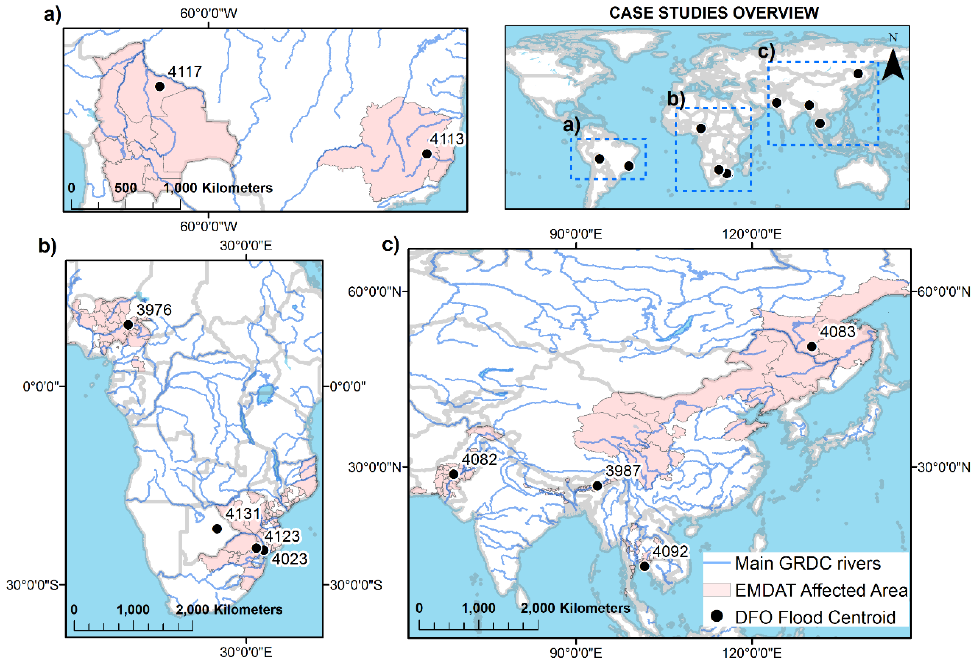
2.1. Flood Disaster Databases and Case Studies


| Case Study ID | DFO ID # | Country | Detailed Locations | Began | Ended | Cause | DFO Centroid X | DFO Centroid Y | Upstream Area (x1000 km2) |
|---|---|---|---|---|---|---|---|---|---|
| 1 | 3976 | Nigeria, Cameroon | Adamawa state, eastern Nigeria, Kogi state | 25/08/2012 | 26/09/2012 | Heavy rain, Dam released | 12.1089 | 9.30166 | 170 |
| 2 | 3987 | India | Assam, north-eastern India | 19/09/2012 | 15/10/2012 | Monsoonal rain | 93.6379 | 26.8031 | 469 |
| 3 | 4023 | Mozambique, Namibia, Malawi, Zimbabwe | Limpopo river basin in southern province of Gaza, Zimbabwe along border with South Africa, KwaZulu-Natal in South Africa, northern Mozambique | 17/01/2013 | 4/3/2013 | Heavy rain | 32.6773 | −24.8006 | 329 |
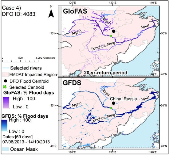
| 4 | 4083 | China, Russia | NE China, including Fushun City, Liaoning Province | 7/8/2013 | 14/10/2013 | Heavy rain | 130.272 | 50.5323 | 914 |
| 5 | 4082 | Pakistan | Punjab, Sindh, and Baluchistan | 7/8/2013 | 21/08/2013 | Monsoonal rain | 69.1065 | 28.7404 | 742 |
| 6 | 4092 | Thailand | 26 of 77 provinces | 30/09/2013 | 14/10/2013 | Monsoonal rain | 101.694 | 13.0819 | 1.2 |
| 7 | 4113 | Brazil | Southeast states of Minas Gerais, and Espirito Santo | 23/12/2013 | 04/01/2014 | Heavy rain | −41.9423 | −18.9538 | 81 |
| 8 | 4117 | Bolivia | La Paz, Beni, Santa Cruz and Cochabamba; north-eastern Bolivia | 10/1/2014 | 1/5/2014 | Heavy rain | −64.0135 | −13.3888 | 161 |
| 9 | 4123 | Mozambique | Johannesburg, Kliptown, Soweto, eastern South Africa, Zimbabwe, and SE Mozambique, Kruger, Incomati River | 24/02/2014 | 10/3/2014 | Heavy rain | 31.5459 | −24.4459 | 54 |
| 10 | 4131 | South Africa, Namibia, Botswana, Zimbabwe | SADC region, Zambezi River Limpopo, Mpumalanga, North West, Gauteng, KwaZulu Natal | 1/3/2014 | 30/03/2014 | Heavy rain | 25.6074 | −21.5153 | 223 |
2.2. Satellite-Derived Global Flood Monitoring
2.2.1. GFDS Flood Magnitude
2.2.2. MODIS Flood Maps
2.2.3. GloFAS Flood Forecasting
3. Methods
3.1. Flood Maps
3.2. Flood Detection Indicator
3.3. Data Agreement at Specific Locations
4. Results
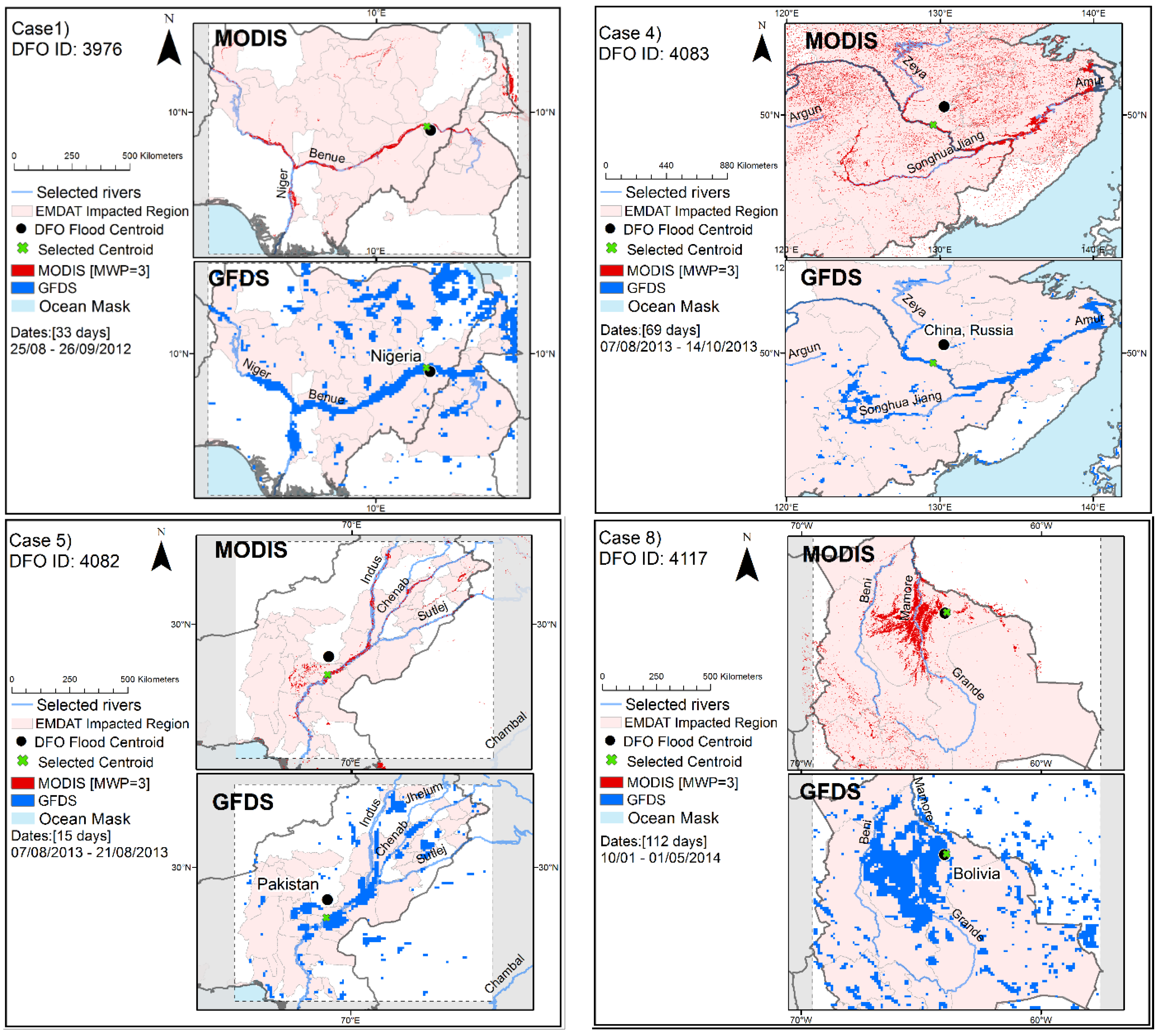
4.1. Comparison of the GFDS and MODIS Flood Maps

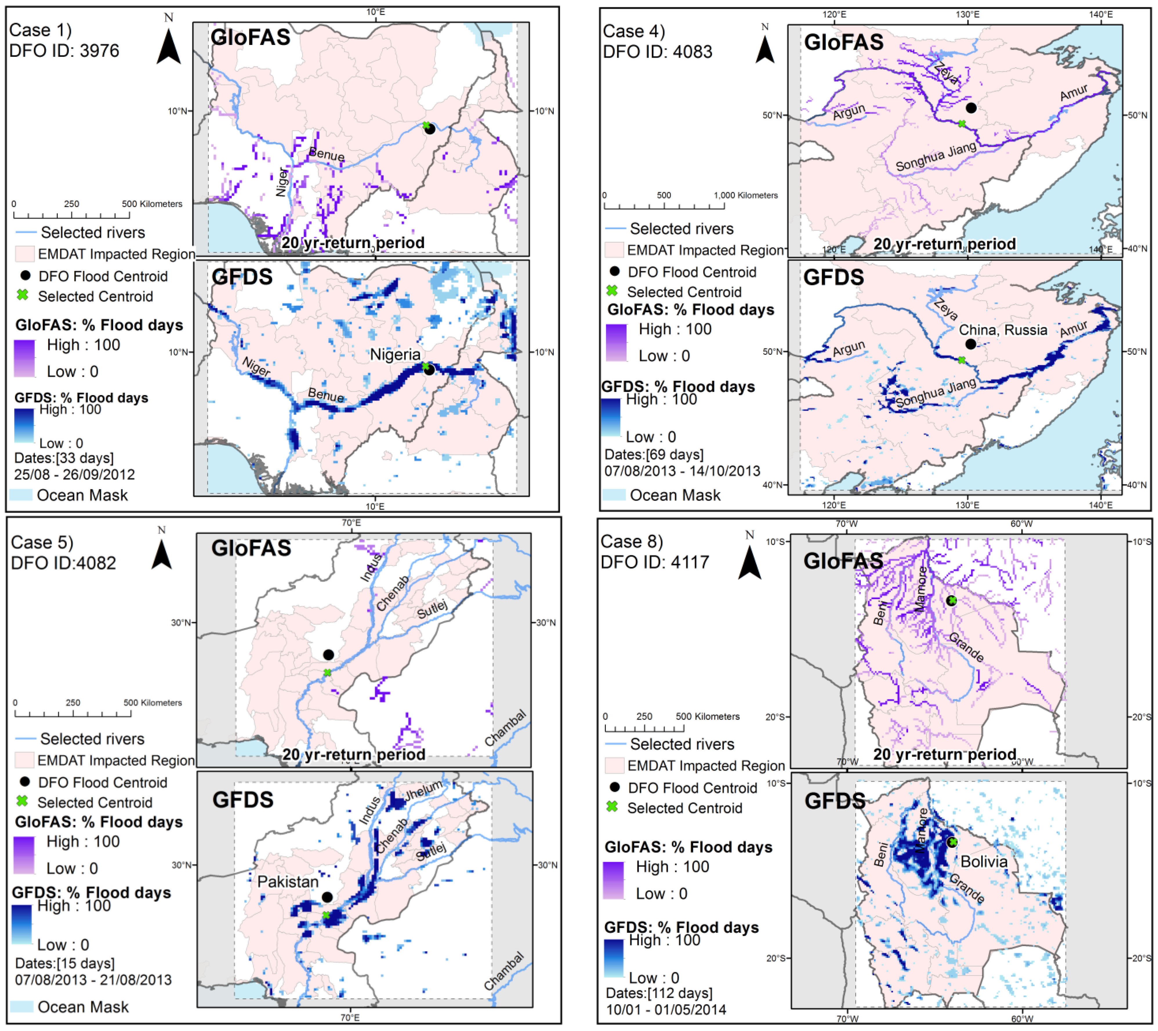
4.2. Comparison of the GFDS and GloFAS
4.2.1. Flood Duration

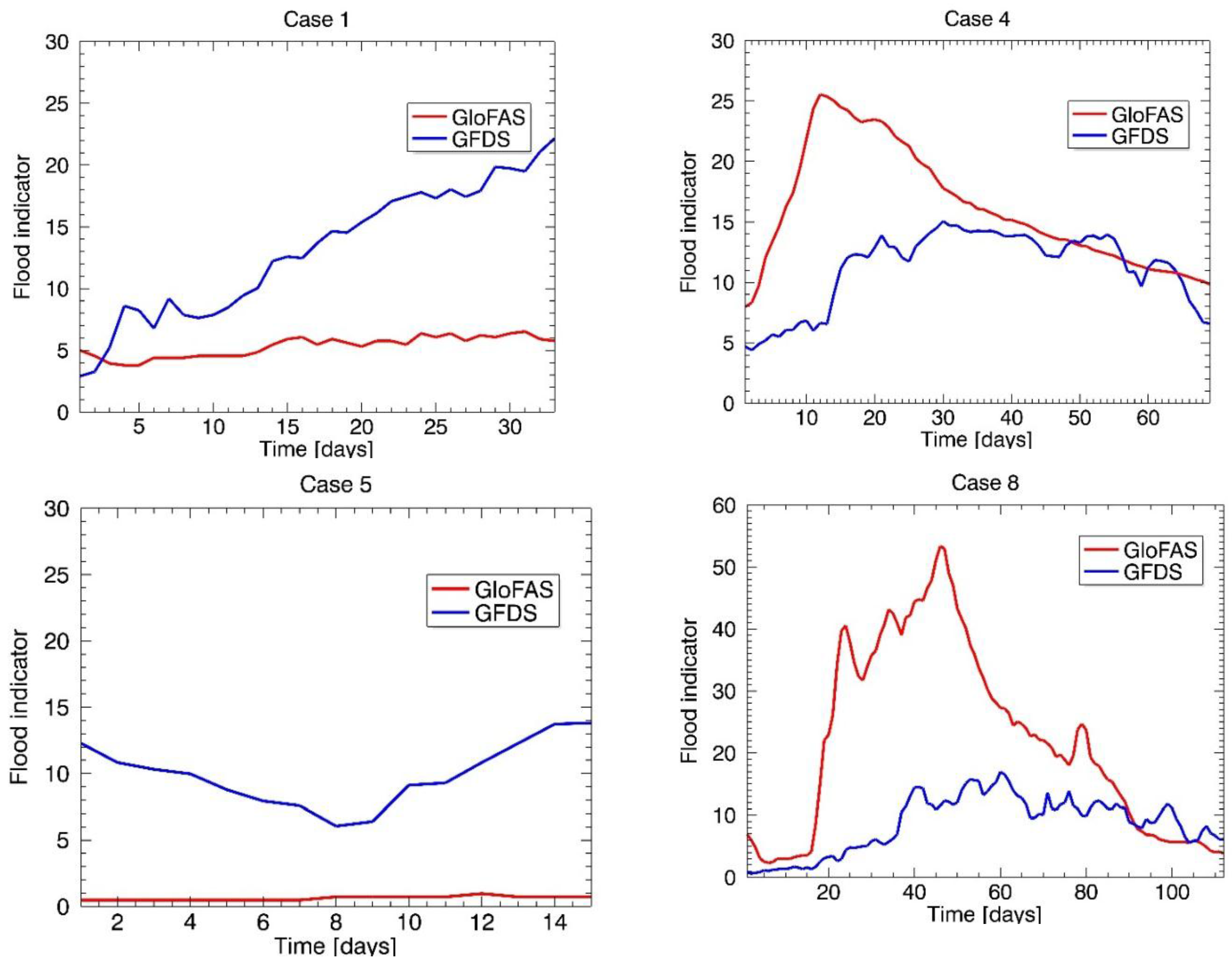
4.2.2. Flood Indicator Time Series

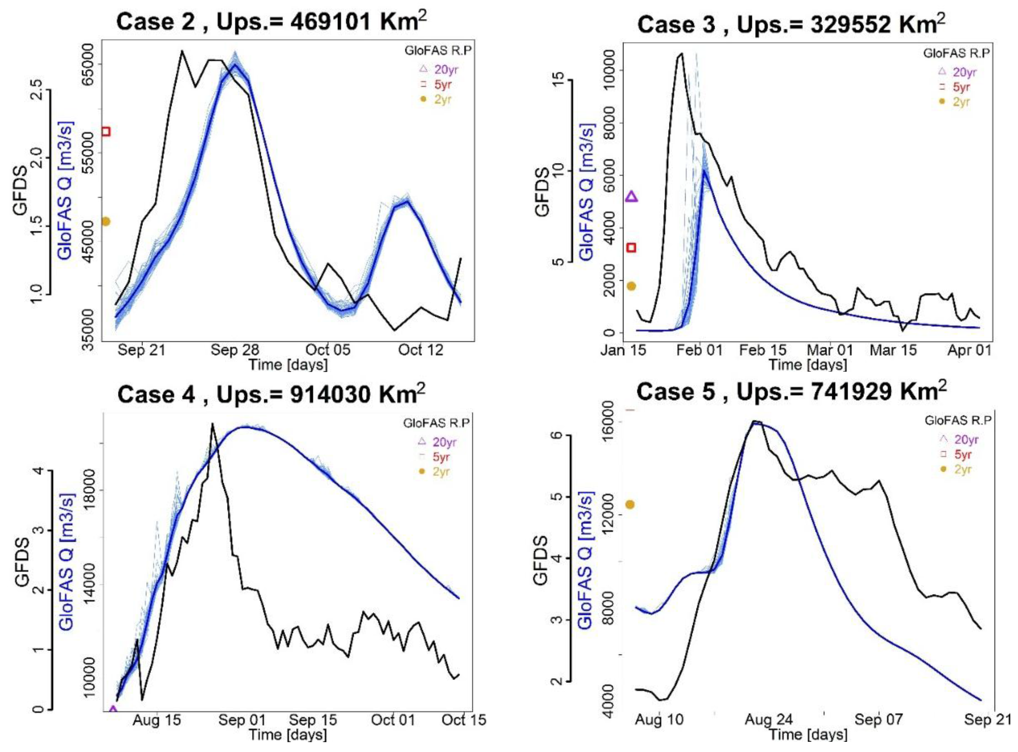
4.2.3. Onset and Evolution of the Flood Events

| Case Study | Forecasted * | GFDS Detected | MODIS Detected | Time Series. Captured | Correlation Time Series | Comments |
|---|---|---|---|---|---|---|
| 1 | Partially | Yes | Yes | Yes if extended | 0.33 | GFDS capture flood in Benue river due to water released from dam in Cameroon, while GloFAS not fully forecasted the intensity of the event, aggravated by the release of the water from the dam. Longer reported date needed to fully capture the event. DFO centroid within the impacted area. |
| 2 | Yes | Partially | Yes | Yes | 0.78 | Flood extent match, but not very strong signal in GFDS along all the Brahmaputra. DFO centroid within the impacted area. |
| 3 | Yes | Yes | Partially | Yes | 0.86 | Agreement mainly on the Limpopo and Zambezi rivers. Larger floods were detected and forecasted further upstream. DFO centroid within the impacted area. |
| 4 | Yes | Yes | Yes | Yes | 0.54 | Flood extent match in main Argun, Songhua Jiang and Amur river, but with disagreement in Zeya. DFO centroid within the impacted area, but it is far from main river. |
| 5 | Partially (5 yr-return level) | Yes | Yes | Yes if extended | 0.61 | Flood extent match in main Indus and Chenab rivers. Extended dates were needed to fully capture the event. DFO centroid outside impacted area, and far from main river. |
| 6 | Yes | Yes | Yes | Yes if extended | 0.82 | Flood extent match, noise in GFDS signal due to proximity to coast. Extended dates needed to fully capture the event. DFO centroid within the impacted area |
| 7 | Partially | Scattered | No | No | −0.2 | Scatter flooded area in GFDS and there was no MFM detection. DFO centroid within the impacted area. |
| 8 | Yes | Yes | Yes | Yes | 0.35 | Clear flooded extent was observed in Beni and Grande rivers. DFO centroid within the impacted area. |
| 9 | No | Scattered | Scattered | Yes if extended | 0.84 | GloFAS forecasted for Limpopo, Zambezi and Shire rivers. Scattered GFDS flood extent was observed, and do not match impacted area. There was no MFP detection. Extended dates are needed to fully capture the event. DFO centroid outside the impacted area, and far from main river. |
| 10 | Partially | Scattered | Scattered | Yes | 0.12 | There is spatial disagreement, especially in Namibia and Botswana. Namibia flooded extent matched with the Great Escarpment area and is during the rainy season. There is noise in GFDS signal due to proximity to coast. No MWP detection. DFO centroid outside the impacted area, and far from main river. |
5. Discussion
5.1. Known Limitations
5.2. Implications for Decision Makers
6. Conclusions and Future Research Direction
Supplementary Materials
Acknowledgments
Author Contributions
Conflicts of Interest
References
- Centre for Research on the Epidemiology of Disasters (CRED). The Human Cost of Natural Disasters 2015: A Global Perspective. Available online: http://reliefweb.int/report/world/human-cost-natural-disasters-2015-global-perspective (accessed on 25 August 2015).
- Making Development Sustainable: The Future of Disaster Risk Management. Available online: http://www.preventionweb.net/english/hyogo/gar/2015/en/gar-pdf/GAR2015_EN.pdf (accessed on 25 August 2015).
- De Groeve, T.; Thielen, J.; Brakenridge, R.; Adler, R.; Alfieri, L.; Kull, D.; Lindsay, F.; Imperiali, O.; Pappenberger, F.; Rudari, R.; et al. Joining forces in a global flood partnership. Bull. Am. Meteorol. Soc. 2014. [Google Scholar] [CrossRef]
- Alfieri, L.; Burek, P.; Dutra, E.; Krzeminski, B.; Muraro, D.; Thielen, J.; Pappenberger, F. GloFAS—Global ensemble streamflow forecasting and flood early warning. Hydrol. Earth Syst. Sci. 2013, 17, 1161–1175. [Google Scholar] [CrossRef] [Green Version]
- Van Beek, L.P.H.; Bierkens, M.F.P. The Global Hydrological Model PCR-GLOBWB: Conceptualization, Parameterization and Verification. Available online: http://vanbeek.geo.uu.nl/suppinfo/vanbeekbierkens2009.pdf (accessed on 25 August 2015).
- Yamazaki, D.; Kanae, S.; Kim, H.; Oki, T. A physically based description of floodplain inundation dynamics in a global river routing model. Water Resour. Res. 2011. [Google Scholar] [CrossRef]
- Wu, H.; Adler, R.F.; Tian, Y.; Huffman, G.J.; Li, H.; Wang, J. Real-time global flood estimation using satellite-based precipitation and a coupled land surface and routing model. Water Resour. Res. 2014, 50, 2693–2717. [Google Scholar] [CrossRef]
- Stephens, E.; Coughlan de Perez, E.; Kruczkiewicz, A.; Boyd, E.; Suarez, P. Forescast-Based Action. A Co-Produced Research Roadmap for Forecast-Based Pre-Emptive Action. Available online: http://www.climatecentre.org/downloads/files/Stephens%20et%20al.%20Forecast-based%20Action%20SHEAR%20Final%20Report.pdf (accessed on 25 August 2015).
- Coughlan de Perez, E.; van den Hurk, B.; van Aalst, M.K.; Jongman, B.; Klose, T.; Suarez, P. Forecast-based financing: An approach for catalyzing humanitarian action based on extreme weather and climate forecasts. Nat. Hazards Earth Syst. Sci. 2015, 15, 895–904. [Google Scholar] [CrossRef]
- Hannah, D.M.; Demuth, S.; van Lanen, H.A.J.; Looser, U.; Prudhomme, C.; Rees, G.; Stahl, K.; Tallaksen, L.M. Large-scale river flow archives: importance, current status and future needs. Hydrol. Process. 2011, 25, 1191–1200. [Google Scholar] [CrossRef]
- Global Runoff Data Centre (GRDC). The River Discharge Time Series, Koblenz, Germany: Federal Institute of Hydrology (BfG). Available online: http://grdc.bafg.de (accessed on 25 August 2015).
- Schumann, G.; Bates, P.D.; Horritt, M.S.; Matgen, P.; Pappenberger, F. Progress in integration of remote sensing-derived flood extent and stage data and hydraulic models. Rev. Geophys. 2009. [Google Scholar] [CrossRef]
- Smith, L.C. Satellite remote sensing of river inundation area, stage, and discharge: A review. Hydrol. Process. 1997, 11, 1427–1439. [Google Scholar] [CrossRef]
- Brakenridge, G.R.; Nghiem, S.V.; Anderson, E.; Mic, R. Orbital microwave measurement of river discharge and ice status. Water Resour. Res. 2007. [Google Scholar] [CrossRef]
- Revilla-Romero, B.; Thielen, J.; Salamon, P.; de Groeve, T.; Brakenridge, G.R. Evaluation of the satellite-based global flood detection system for measuring river discharge: Influence of local factors. Hydrol. Earth Syst. Sci. 2014, 18, 4467–4484. [Google Scholar] [CrossRef] [Green Version]
- Tarpanelli, A.; Brocca, L.; Lacava, T.; Melone, F.; Moramarco, T.; Faruolo, M.; Pergola, N.; Tramutoli, V. Toward the estimation of river discharge variations using MODIS data in ungauged basins. Remote Sens. Environ. 2013, 136, 47–55. [Google Scholar] [CrossRef]
- Gleason, C.J.; Smith, L.C. Toward global mapping of river discharge using satellite images and at-many-stations hydraulic geometry. Proc. Natl. Acad. Sci. 2014, 111, 4788–4791. [Google Scholar] [CrossRef] [PubMed]
- Birkinshaw, S.J.; Moore, P.; Kilsby, C.G.; O’Donnell, G.M.; Hardy, A.J.; Berry, P.A.M. Daily discharge estimation at ungauged river sites using remote sensing. Hydrol. Process. 2014, 28, 1043–1054. [Google Scholar] [CrossRef]
- Revilla-Romero, B.; Beck, H.E.; Burek, P.; Salamon, P.; de Roo, A.; Thielen, J. Filling the gaps: Calibrating a rainfall-runoff model using satellite-derived surface water extent. Remote Sens. Environ. 2015, 171, 118–131. [Google Scholar] [CrossRef]
- Wanders, N.; Karssenberg, D.; de Roo, A.; de Jong, S.M.; Bierkens, M.F.P. The suitability of remotely sensed soil moisture for improving operational flood forecasting. Hydrol. Earth Syst. Sci. 2014, 18, 2343–2357. [Google Scholar] [CrossRef]
- Hirpa, F.A.; Gebremichael, M.; Hopson, T.M.; Wojick, R.; Lee, H. Assimilation of satellite soil moisture retrievals into a hydrologic model for improving river discharge. In Remote Sensing of the Terrestrial Water Cycle; Lakshmi, V., Alsdorf, D., Anderson, M., Biancamaria, S., Cosh, M., Entin, J., Huffman, G., Kustas, W., van Oevelen, P., Painter, T., Parajka, J., Rodell, T., Rüdiger, C., Eds.; John Wiley & Sons Inc: Hoboken, NJ, USA, 2014; pp. 319–329. [Google Scholar]
- Hostache, R.; Matgen, P.; Schumann, G.; Puech, C.; Hoffmann, L.; Pfister, L. Water level estimation and reduction of hydraulic model calibration uncertainties using satellite SAR images of floods. IEEE Trans. Geosci. Remote Sens. 2009, 47, 431–441. [Google Scholar] [CrossRef]
- Giustarini, L.; Matgen, P.; Hostache, R.; Montanari, M.; Plaza, D.; Pauwels, V.R.N.; de Lannoy, G.J.M.; de Keyser, R.; Pfister, L.; Hoffmann, L.; et al. Assimilating SAR-derived water level data into a hydraulic model: A case study. Hydrol. Earth Syst. Sci. 2011, 15, 2349–2365. [Google Scholar] [CrossRef] [Green Version]
- Di Baldassarre, G.; Schumann, G.; Bates, P.D. A technique for the calibration of hydraulic models using uncertain satellite observations of flood extent. J. Hydrol. 2009, 367, 276–282. [Google Scholar] [CrossRef]
- Domeneghetti, A.; Tarpanelli, A.; Brocca, L.; Barbetta, S.; Moramarco, T.; Castellarin, A.; Brath, A. The use of remote sensing-derived water surface data for hydraulic model calibration. Remote Sens. Environ. 2014, 149, 130–141. [Google Scholar] [CrossRef]
- Dung, N.V.; Merz, B.; Bárdossy, A.; Thang, T.D.; Apel, H. Multi-objective automatic calibration of hydrodynamic models utilizing inundation maps and gauge data. Hydrol. Earth Syst. Sci. 2011, 15, 1339–1354. [Google Scholar] [CrossRef] [Green Version]
- Sun, W.; Ishidaira, H.; Bastola, S. Towards improving river discharge estimation in ungauged basins: Calibration of rainfall-runoff models based on satellite observations of river flow width at basin outlet. Hydrol. Earth Syst. Sci. 2010, 14, 2011–2022. [Google Scholar] [CrossRef]
- Kundu, S.; Aggarwal, S.P.; Kingma, N.; Mondal, A.; Khare, D. Flood monitoring using microwave remote sensing in a part of Nuna river basin, Odisha, India. Nat. Hazards 2015, 76, 123–138. [Google Scholar] [CrossRef]
- Schumann, G.J.P.; Moller, D.K. Microwave remote sensing of flood inundation. Phys. Chem. Earth 2015. [Google Scholar] [CrossRef]
- Birkett, C.M.; Mertes, L.A.K.; Dunne, T.; Costa, M.H.; Jasinski, M.J. Surface water dynamics in the Amazon Basin: Application of satellite radar altimetry. J. Geophys. Res. 2002. [Google Scholar] [CrossRef]
- Getirana, A.C.V. Integrating spatial altimetry data into the automatic calibration of hydrological models. J. Hydrol. 2010, 387, 244–255. [Google Scholar] [CrossRef]
- Sun, W.; Ishidaira, H.; Bastola, S. Calibration of hydrological models in ungauged basins based on satellite radar altimetry observations of river water level. Hydrol. Process. 2012, 26, 3524–3537. [Google Scholar] [CrossRef]
- Allen, G.H.; Pavelsky, T.M. Patterns of river width and surface area revealed by the satellite-derived North American River Width data set. Geophys. Res. Lett. 2015, 42, 395–402. [Google Scholar] [CrossRef]
- Durand, M.; Andreadis, K.M.; Alsdorf, D.E.; Lettenmaier, D.P.; Moller, D.; Wilson, M. Estimation of bathymetric depth and slope from data assimilation of swath altimetry into a hydrodynamic model. Geophys. Res. Lett. 2008. [Google Scholar] [CrossRef]
- Callow, J.N.; Boggs, G.S. Studying reach-scale spatial hydrology in ungauged catchments. J. Hydrol. 2013, 496, 31–46. [Google Scholar] [CrossRef]
- Kugler, Z.; de Groeve, T. The Global Flood Detection System; Office for Official Publications of the European Communities: Seat, Luxembourg, 2007. [Google Scholar]
- Khan, S.I.; Hong, Y.; Gourley, J.J.; Khattak, M.U.; de Groeve, T. Multi-sensor imaging and space-ground cross-validation for 2010 flood along Indus River, Pakistan. Remote Sens. 2014, 6, 2393–2407. [Google Scholar] [CrossRef] [Green Version]
- Jongman, B.; Wagemaker, J.; Revilla-Romero, B.; Coughlan de Perez, E. Early flood detection for rapid humanitarian response: Harnessing big data from near real-time satellite and twitter signals. ISPRS Int. J. Geo-Inf. 2015, 4, 2246–2266. [Google Scholar] [CrossRef]
- Nigro, J.; Slayback, D.; Policelli, F.; Brakenridge, G.R. NASA/DFO MODIS Near Real-Time (NRT) Global Flood Mapping Product Evaluation of Flood and Permanent Water Detection. Available online: http://oas.gsfc.nasa.gov/floodmap/documents/NASAGlobalNRTEvaluationSummary_v4.pdf (accessed on 25 August 2015).
- Brakenridge, R.; Anderson, E. Modis-based flood detection, mapping and measurement: The potential for operational hydrological applications. In Transboundary Floods: Reducing Risks Through Flood Management; Marsalek, J., Stancalie, G., Balint, G., Eds.; Springer Netherlands: Dordrecht, The Netherlands, 2006; pp. 1–12. [Google Scholar]
- Memon, A.A.; Muhammad, S.; Rahman, S.; Haq, M. Flood monitoring and damage assessment using water indices: A case study of Pakistan flood-2012. Egypt. J. Remote Sens. Space Sci. 2015, 18, 99–106. [Google Scholar] [CrossRef]
- Huang, C.; Chen, Y.; Wu, J. Mapping spatio-temporal flood inundation dynamics at large riverbasin scale using time-series flow data and MODIS imagery. Int. J. Appl. Earth Obs. Geoinf. 2014, 26, 350–362. [Google Scholar] [CrossRef]
- Sakamoto, T.; Van Nguyen, N.; Kotera, A.; Ohno, H.; Ishitsuka, N.; Yokozawa, M. Detecting temporal changes in the extent of annual flooding within the Cambodia and the Vietnamese Mekong Delta from MODIS time-series imagery. Remote Sens. Environ. 2007, 109, 295–313. [Google Scholar] [CrossRef]
- Brakenridge, R.G.; Cohen, S.; Kettner, A.J.; De Groeve, T.; Nghiem, S.V.; Syvitski, J.P.M.; Fekete, B.M. Calibration of satellite measurements of river discharge using a global hydrology model. J. Hydrol. 2012, 475, 123–136. [Google Scholar] [CrossRef]
- Khan, S.I.; Hong, Y.; Wang, J.; Yilmaz, K.K.; Gourley, J.J.; Adler, R.F.; Brakenridge, G.R.; Policell, F.; Habib, S.; Irwin, D. Satellite remote sensing and hydrologic modeling for flood inundation mapping in Lake Victoria Basin: Implications for hydrologic prediction in ungauged basins. IEEE Trans. Geosci. Remote Sens. 2011, 49, 85–95. [Google Scholar] [CrossRef]
- Chapman, B.; McDonald, K.; Shimada, M.; Rosenqvist, A.; Schroeder, R.; Hess, L. Mapping regional inundation with spaceborne L-Band SAR. Remote Sens. 2015, 7, 5440–5470. [Google Scholar] [CrossRef]
- Brakenridge, G.R. Global Active Archive of Large Flood Events, Dartmouth Flood Observatory. Available online: http://floodobservatory.colorado.edu/Archives/index.html (accessed on 25 August 2015).
- Guha-Sapir, D.; Below, R.; Hoyois, P. EM-DAT: International Disaster Database. Available online: www.emdat.be (accessed on 25 August 2015).
- De Groeve, T.; Schmidt, R.; Raeva, L.; Dittrich, D.; Musilek, J.; Reland, M.; Vainio, T.; Nussbaum, R.; Thieken, A.; Kreibich, H.; et al. Guidance for Recording and Sharing Disaster Damage and Loss Data: Towards the Development of Operational Indicators to Translate the Sendai Framework into Action. Available online: http://publications.jrc.ec.europa.eu/repository/handle/JRC95505 (accessed on 25 August 2015).
- World Meteorological Organization (WMO). First Technical Workshop on Standards for Hazard Monitoring, Data, Metadata and Analysis to Support Risk Assessment; WMO: Geneva, Switzerland, 2013.
- NASA Tropical Rainfall Measuring Mission (TRMM). Available online: http://trmm.gsfc.nasa.gov (accessed on 25 August 2015).
- NASA Advanced Microwave Scanning Radiometer for Earth Observation System (AMSR-E). Available online: http://aqua.nasa.gov/about/instrument_amsr.php (accessed on 25 August 2015).
- JAXA Advanced Microwave Scanning Radiometer 2 (AMSR2). Available online: http://suzaku.eorc.jaxa.jp/GCOM_W/w_amsr2/whats_amsr2.html (accessed on 25 August 2015).
- NASA Global Precipitation Measurement (GPM). Available online: http://pmm.nasa.gov/GPM (accessed on 25 August 2015).
- Buizza, R.; Bidlot, J.R.; Wedi, N.; Fuentes, M.; Hamrud, M.; Holt, G.; Vitart, F. The new ECMWF VAREPS (Variable Resolution Ensemble Prediction System). Q. J. R. Meteorol. Soc. 2007, 133, 681–695. [Google Scholar] [CrossRef]
- Balsamo, G.; Beljaars, A.; Scipal, K.; Viterbo, P.; van den Hurk, B.; Hirschi, M.; Betts, A.K. A revised hydrology for the ECMWF model: Verification from field site to terrestrial water storage and impact in the integrated forecast system. J. Hydrometeorol. 2009, 10, 623–643. [Google Scholar] [CrossRef]
- Dutra, E.; Balsamo, G.; Viterbo, P.; Miranda, P.M.A.; Beljaars, A.; Schär, C.; Elder, K. An improved snow scheme for the ECMWF land surface model: Description and offline validation. J. Hydrometeorol. 2010, 11, 899–916. [Google Scholar] [CrossRef]
- Burek, P.; van der Knijff, J.; de Roo, A. LISFLOOD—Distributed Water Balance and Flood Simulation Model Revised User Manual; Technical Report for JRC: Ispra, Italy, 2013. [Google Scholar]
- Van Der Knijff, J.M.; Younis, J.; De Roo, A.P.J. LISFLOOD: A GIS-based distributed model for river basin scale water balance and flood simulation. Int. J. Geogr. Inf. Sci. 2010, 24, 189–212. [Google Scholar] [CrossRef]
- Chow, V.T.; Maidment, D.R.; Mays, L.W. Applied Hydrology; Tata McGraw-Hill Education: New York, NY, USA, 1988. [Google Scholar]
- Hirpa, F.A.; Salamon, P.; Alfieri, L.; Thielen, J.; Zsoter, E.; Pappenberger, F. The effect of reference climatology on global flood forecasting. J. Hydrometeorol. 2015, submitted. [Google Scholar]
- Dottori, F.; Salamon, P.; Bianchi, A.; Alfieri, L.; Feyen, L. Development and evaluation of a framework for global flood hazard mapping. Adv. Water Resour. 2015. under review. [Google Scholar]
- Dee, D.P.; Uppala, S.M.; Simmons, A.J.; Berrisford, P.; Poli, P.; Kobayashi, S.; Andrae, U.; Balmaseda, M.A.; Balsamo, G.; Bauer, P.; et al. The ERA-Interim reanalysis: Configuration and performance of the data assimilation system. Q. J. R. Meteorol. Soc. 2011, 137, 553–597. [Google Scholar] [CrossRef]
- Dottori, F.; Todini, E. Developments of a flood inundation model based on the cellular automata approach: Testing different methods to improve model performance. Phys. Chem. Earth 2011, 36, 266–280. [Google Scholar] [CrossRef]
- PDNA Nigeria Post Disaster Need Assessment 2012 floods. A report by The Federal Government of Nigeria. Available online: https://www.gfdrr.org/sites/gfdrr/files/NIGERIA_PDNA_PRINT_05_29_2013_WEB.pdf (accessed on 25 August 2015).
- Hirpa, F.A.; Hopson, T.M.; De Groeve, T.; Brakenridge, G.R.; Gebremichael, M.; Restrepo, P.J. Upstream satellite remote sensing for river discharge forecasting: Application to major rivers in South Asia. Remote Sens. Environ. 2013, 131, 140–151. [Google Scholar] [CrossRef]
- Brakenridge, G.; De Groeve, T.; Cohen, S.; Nghiem, S.V. River Watch, Version 2: Satellite River Discharge and Runoff Measurements: Technical Summary. Available online: http://floodobservatory.colorado.edu/SatelliteGaugingSites/technical.html (accessed on 25 August 2015).
- Alfieri, L.; Thielen, J. A European precipitation index for extreme rain-storm and flash flood early warning. Meteorol. Appl. 2015, 22, 3–13. [Google Scholar] [CrossRef]
- Raynaud, D.; Thielen, J.; Salamon, P.; Burek, P.; Anquetin, S.; Alfieri, L. A dynamic runoff co-efficient to improve flash flood early warning in Europe: Evaluation on the 2013 central European floods in Germany. Meteorol. Appl. 2015, 22, 410–418. [Google Scholar] [CrossRef]
- Modrick, T.M.; Graham, R.; Shamir, E.; Jubach, R.; Spencer, C.R.; Sperfslage, J.A.; Georgakakos, K.P. Operational Flash Flood Warning Systems with Global Applicability. Available online: http://www.hrcwater.org/about/aboutpdfs/iEMS2014_Modrick_FlashFloodWarningSystems.pdf (accessed on 25 August 2015).
- Ward, P.J.; Jongman, B.; Salamon, P.; Simpson, A.; Bates, P.; de Groeve, T.; Muis, S.; de Perez, E.C.; Rudari, R.; Trigg, M.A.; Winsemius, H.C. Usefulness and limitations of global flood risk models. Nat. Clim. Change 2015, 5, 712–715. [Google Scholar] [CrossRef]
- De Groeve, T.; Poljansek, K.; Vernaccini, L. Index for Risk Management-INFORM. Concept and Methodology. Version 2015; European Commission: Seat, Luxembourg, 2014. [Google Scholar]
- Bates, P.D.; Neal, J.C.; Alsdorf, D.; Schumann, G.J.P. Observing global surface water flood dynamics. Surv. Geophys. 2014, 35, 839–852. [Google Scholar] [CrossRef]
- Pavelsky, T.M.; Durand, M.T.; Andreadis, K.M.; Edward Beighley, R.; Paiva, R.C.D.; Allen, G.H.; Miller, Z.F. Assessing the potential global extent of SWOT river discharge observations. J. Hydrol. 2014, 519, 1516–1525. [Google Scholar] [CrossRef]
- Schumann, G.J.; Bates, P.D.; Di Baldassarre, G.; Mason, D.C. The use of radar imagery in riverine flood inundation studies. In Fluvial Remote Sensing for Science and Management; John Wiley & Sons: Chichester, UK, 2012; pp. 115–140. [Google Scholar]
- Westerhoff, R.S.; Kleuskens, M.P.H.; Winsemius, H.C.; Huizinga, H.J.; Brakenridge, G.R.; Bishop, C. Automated global water mapping based on wide-swath orbital synthetic-aperture radar. Hydrol. Earth Syst. Sci. 2013, 17, 651–663. [Google Scholar] [CrossRef]
- UNITAR/UNOSAT Overview of flood waters in Mangla area, and Northern Punjab (Pakistan). Analysis with SENTINEL-1 and Landsat-8/. Available online: http://unosat-maps.web.cern.ch/unosat-maps/PK/FL20150723PAK/UNOSAT_A3_Multan_200k_portrait_20150727.pdf (accessed on 25 August 2015).
- Posner, A.J.; Georgakakos, K.P.; Shamir, E. MODIS inundation estimate assimilation into soil moisture accounting hydrologic model: A case study in Southeast Asia. Remote Sens. 2014, 6, 10835–10859. [Google Scholar] [CrossRef]
© 2015 by the authors; licensee MDPI, Basel, Switzerland. This article is an open access article distributed under the terms and conditions of the Creative Commons Attribution license (http://creativecommons.org/licenses/by/4.0/).
Share and Cite
Revilla-Romero, B.; Hirpa, F.A.; Pozo, J.T.-d.; Salamon, P.; Brakenridge, R.; Pappenberger, F.; De Groeve, T. On the Use of Global Flood Forecasts and Satellite-Derived Inundation Maps for Flood Monitoring in Data-Sparse Regions. Remote Sens. 2015, 7, 15702-15728. https://0-doi-org.brum.beds.ac.uk/10.3390/rs71115702
Revilla-Romero B, Hirpa FA, Pozo JT-d, Salamon P, Brakenridge R, Pappenberger F, De Groeve T. On the Use of Global Flood Forecasts and Satellite-Derived Inundation Maps for Flood Monitoring in Data-Sparse Regions. Remote Sensing. 2015; 7(11):15702-15728. https://0-doi-org.brum.beds.ac.uk/10.3390/rs71115702
Chicago/Turabian StyleRevilla-Romero, Beatriz, Feyera A. Hirpa, Jutta Thielen-del Pozo, Peter Salamon, Robert Brakenridge, Florian Pappenberger, and Tom De Groeve. 2015. "On the Use of Global Flood Forecasts and Satellite-Derived Inundation Maps for Flood Monitoring in Data-Sparse Regions" Remote Sensing 7, no. 11: 15702-15728. https://0-doi-org.brum.beds.ac.uk/10.3390/rs71115702