3.1. Soil Properties and Soil Quality
The mean value of all the soil properties from the Migda site is presented in
Table 1, along with their SDs and significance values. The results of the three land uses show significant differences in all soil properties except for P. Significantly higher values of SH and SOM were found in the abandoned agricultural field with no grazing than in the other two land uses. In the agro-pastoral agricultural field, significantly higher values of HC, NH
4, and K were found than in the other two land uses.
Table 2 represents the respective Pearson correlation coefficients (R) for the measured soil properties. The results indicate soil properties with significant correlations (R ≥ 0.5, bold numbers) and with highly significant coefficient correlations (R > ±0.8 bold numbers with (*)). To avoid properties that could be considered as redundant, the multivariate correlation was tested for R ≥ ±0.8. Later, the soil properties with a high factor loading were eliminated from the SQI. High correlations were found between HC and SH and NH
4 (R = −0.83 and R = 0.79;
p > 0.01, respectively) and between SH and NO
3, and K (R = −0.92 and R = −0.88;
p > 0.01, respectively). In addition, a high correlation was found between K and NH
4 (R = 0.88;
p = 0.01).
The results of the soil properties from the Schäfertal site are shown in
Table 3. The three land uses show significant differences in all soil properties except for P. Significantly higher values of SH, SOM, PAC and NH
4+ were found in the forest than in the agricultural land uses. In the agricultural land uses, significantly higher values of pH, EC, NO
3 and K were found than in the forest. Significant differences were found between the two agricultural fields in AWC, SH, and pH. The higher pH value in the fertilized agricultural field than in the unfertilized field might be explained by the urea application several days before the campaign [
69]. In addition, significant differences in soil texture were observed between the three land uses. The soil in the forest had higher clay content, which is related to the ability to retain nutrients (higher cation exchange capacity) and to bind more organic matter.
Table 4 represents the Pearson correlations. High negative correlations were found between SOM and pH and NO
3 (R = −0.92; R = −0.79,
p = 0.01, respectively). In addition, a positive correlation was found between EC and NO
3 (R = 0.85;
p = 0.01).
Table 1.
Soil quality properties for the Migda site, Israel, with the following treatments: (A) abandoned field no grazing; (B) agro-pastoral grazing; and (C) abandoned field with grazing. Statistics include: average value, standard deviation (SD), and indication of significant differences between treatments represented with small letters (a, b, c).
| Soil Properties | Abandoned Field No Grazing | Agro-Pastoral Grazing | Abandoned Field with Grazing |
|---|
| Sand (%) (0.063–2.0) | 49.12 ± 1.34a | 44.32 ± 1.14b | 39.52 ± 4.15c |
| Silt (%) (0.002–0.063) | 37.08 ± 1.09a | 38.68 ± 1.95a | 38.08 ± 3.11a |
| Clay (%) (<0.002) | 13.8 ± 0.44c | 17.0 ± 1.01b | 22.4 ± 2.88a |
| AWC (%) | 0.126 ± 0.03a | 0.120 ± 0.01a | 0.102 ± 0.02b |
| HC (mm/h) | 0.39 ± 0.08b | 0.59 ± 0.106a | 0.288 ± 0.05c |
| SH (psi) | 316.16 ± 5.18a | 159.05 ± 12.08c | 299.65 ± 8.43b |
| SOM (%) | 4.85 ± 0.509a | 3.477 ± 0.306b | 2.814 ± 0.49c |
| PAC | 860.49 ± 159.9a | 889.74 ± 116.65a | 724.24 ± 185.07b |
| pH | 7.39 ± 0.05a | 7.32 ± 0.054a | 7.59 ± 0.058b |
| EC (µS/cm) | 0.527 ± 0.09a | 0.535 ± 0.042a | 0.363 ± 0.06b |
| N-NH4+ (mg/100gr) | 3.30 ± 1.01b | 15.895 ± 2.63a | 4.76 ± 1.17b |
| N-NO3 (mg/100gr) | 12.21 ± 2.45a | 11.68 ± 1.28a | 10.29 ± 1.63b |
| K (ml/100gr) | 12.78 ± 3.45b | 31.15 ± 8.08a | 10.74 ± 1.32b |
| P(mg/100gr) | 22.76 ± 9.25a | 25.155 ± 11.34a | 18.89 ± 7.02a |
Table 2.
Pearson correlation coefficients for the measured soil quality properties in the Migda site, Israel. Bold numbers indicate significant differences with p ≤ 0.05 and bold numbers with (*) indicate highly significant differences with R ≥ 0.8 and p ≤ 0.01.
Table 2.
Pearson correlation coefficients for the measured soil quality properties in the Migda site, Israel. Bold numbers indicate significant differences with p ≤ 0.05 and bold numbers with (*) indicate highly significant differences with R ≥ 0.8 and p ≤ 0.01.
| | AWC (%) | HC (mm/h) | SH (psi) | SOM (Orgs %) | PAC (ppm) | pH | EC (µS/cm) | N(NH4) (mg/kg) | N(NO3) (mi/kg) | K (mg/kg) | P (mg/kg) |
|---|
| AWC (%) | 1.00 | | | | | | | | | | |
| HC (mm/h) | 0.23 | 1.00 | | | | | | | | | |
| SH (psi) | −0.28 | −0.83* | 1.00 | | | | | | | | |
| SOM (Orgs %) | 0.54 | 0.20 | −0.08 | 1.00 | | | | | | | |
| PAC (ppm) | 0.28 | 0.41 | −0.34 | 0.37 | 1.00 | | | | | | |
| pH | −0.36 | −0.49 | 0.55 | −0.44 | −0.40 | 1.00 | | | | | |
| EC (µS/cm) | 0.31 | 0.67 | −0.50 | 0.55 | 0.45 | −0.62 | 1.00 | | | | |
| N(NH4) (mg/kg) | 0.20 | 0.79 | −0.92* | −0.08 | 0.36 | −0.46 | 0.48 | 1.00 | | | |
| N(NO3) (mi/kg) | 0.14 | 0.35 | −0.22 | 0.42 | 0.40 | −0.48 | 0.58 | 0.24 | 1.00 | | |
| K (mg/kg) | 0.20 | 0.74 | −0.88* | 0.08 | 0.32 | −0.51 | 0.54 | 0.88* | 0.31 | 1.00 | |
| P (mg/kg) | 0.18 | 0.45 | −0.26 | 0.26 | 0.25 | −0.23 | 0.68 | 0.41 | 0.42 | 0.35 | 1.00 |
Table 3.
Soil quality properties for the Schäfertal site, Germany, with the following treatments: (A) agriculture 1; (B) agriculture 2; and (C) forest. Statistics include: average value, standard deviation, and indication of significant differences between treatments.
Table 3.
Soil quality properties for the Schäfertal site, Germany, with the following treatments: (A) agriculture 1; (B) agriculture 2; and (C) forest. Statistics include: average value, standard deviation, and indication of significant differences between treatments.
| Soil Properties | Fertilized Agricultural Field | Unfertilized Agricultural Field | Forest |
|---|
| Sand (%) (0.063–2.0) | 19.35 ± 3.87b | 24.07 ± 3.32a | 24.76 ± 3.33a |
| Silt (%) (0.002–0.063) | 61.32 ± 3.56a | 57.31 ± 2.23b | 50.5 ± 2.01c |
| Clay (%) (<0.002) | 19.318 ± 2.74b | 18.62 ± 1.98b | 24.76 ± 1.77a |
| AWC (m/m) | 0.146 ± 0.012a | 0.122 ± 0.019b | 0.104 ± 0.027b |
| SH (psi) | 169.32 ± 18.67c | 260.65 ± 11.02b | 302.11 ± 14.90a |
| SOM (%) | 3.44 ± 0.59b | 3.64 ± 0.51b | 15.96 ± 4.49a |
| PAC (ppm) | 961.75 ± 325.9b | 1048.8 ± 103.11b | 1651.2 ± 142.39a |
| pH | 5.76 ± 0.34a | 5.26 ± 0.26b | 3.72 ± 0.13c |
| EC (µS/cm) | 159.09 ± 26.07a | 168.1 ± 22.88a | 117 ± 28.266b |
| N-NH4+ (mg/100gr) | <0.03c | 0.1 ± 0.036b | 1.54 ± 1.173a |
| N-NO3 (mg/100gr) | 5.05 ± 0.91a | 5.4 ± 1.14a | 1.54 ± 1.17b |
| K (ml/100gr) | 17.83 ± 7.26a | 15.26 ± 5.54a | 6.28 ± 3.09b |
| P (mg/100gr) | 2.28 ± 0.96a | 2.61 ± 0.97a | 4.12 ± 1.901a |
Table 4.
Pearson correlation coefficients for the measured soil quality properties in the Schäfertal site, Germany. Bold numbers indicate significant differences with p ≤ 0.05 and bold numbers with (*) indicate highly significant differences with R ≥ 0.8 and p ≤ 0.01.
Table 4.
Pearson correlation coefficients for the measured soil quality properties in the Schäfertal site, Germany. Bold numbers indicate significant differences with p ≤ 0.05 and bold numbers with (*) indicate highly significant differences with R ≥ 0.8 and p ≤ 0.01.
| | AWC | SH (psi) | SOM (%) | PAC n g/kg | NH4-N (mg/100g) | NO3—N (mg/100g) | pH | EC (µS/cm) | K (mg/100g) | P (mg/100g) |
|---|
| AWC | 1.0 | | | | | | | | | |
| SH (psi) | −0.72 | 1.0 | | | | | | | | |
| SOM (%) | −0.49 | 0.64 | 1.0 | | | | | | | |
| PAC n (mg/kg) | −0.57 | 0.62 | 0.77 | 1.0 | | | | | | |
| NH4+-N (mg/kg) | −0.28 | 0.45 | 0.76 | 0.51 | 1.0 | | | | | |
| NO3−-N (mg/kg) | 0.34 | −0.48 | −0.79 | −0.59 | −0.66 | 1.0 | | | | |
| pH | 0.62 | −0.76 | −0.92* | −0.65 | −0.65 | 0.68 | 1.0 | | | |
| EC (µS/cm) | 0.31 | −0.34 | −0.55 | −0.49 | −0.54 | 0.85* | 0.44 | 1.0 | | |
| K (mg/100g) | 0.19 | −0.44 | −0.56 | −0.34 | −0.33 | 0.68 | 0.61 | 0.53 | 1.0 | |
| P (mg/100g) | −0.21 | 0.39 | 0.49 | 0.618 | 0.05 | −0.11 | −0.45 | 0.07 | −0.12 | 1.0 |
The SQI was developed from the results of the transformed scoring of the soil properties from the two sites. Three PCs that explained 76.71% of the variance of the original data were chosen for an analysis of data redundancy from the Migda site. The PCA indicated three components with eigenvalues ≥1 (
Table 5) that were selected, and the cut-off was placed at the third component. The loading values of the first PC1 (38.35% of variance) indicated HC, SH, pH, EC, and NH
4, and had values within 10% of the highest value. The SH and HC were significantly correlated; therefore, they were associated with the highest loading value, and HC was selected for PC1 (38.35% of variation). For PC2 (28.13% of variation), the loading values were AWC and SOM. They were not significantly correlated, and both were selected for the SQI. For PC3 (10.23% of variation), PAC and NO
3 were within 10% of the highest loading value. The total SQI values for the Migda agricultural site were, for the abandoned agricultural field with no grazing, a score of SQI = 0.48, for the agro-pastoral field, SQI = 0.61, and for the abandoned agricultural field with grazing, SQI = 0.35, with significant differences between all treatments (F = 137.5;
p > 0.01).
Table 5.
Results of the principal component analysis (PCA) of soil properties in the Migda site, Israel. Bold and underlined values indicate underlined factors corresponding to the indicators included in the indices.
Table 5.
Results of the principal component analysis (PCA) of soil properties in the Migda site, Israel. Bold and underlined values indicate underlined factors corresponding to the indicators included in the indices.
| | Scores PC1 | Scores PC2 | Scores PC3 |
|---|
| Eigenvalue | 1.92 | 1.4 | 1.0 |
| Variance | 38.35 | 28.13 | 10.23 |
| Cumulative Variance | 38.35 | 66.48 | 76.71 |
| AWC (%) | −1.13 | −2.12 | −1.06 |
| HC(mm/h) | 6.66 | 1.72 | 0.67 |
| SH(psi) | −5.12 | 3.37 | −1.33 |
| SOM (Orgs % hcl) | −0.61 | −5.59 | −0.10 |
| PAC (ppm) | −1.88 | −1.14 | 3.75 |
| pH | 4.88 | 3.03 | 1.20 |
| EC | 5.60 | 4.30 | −0.99 |
| N(NH4) (mg/kg) | −4.93 | 3.58 | −1.25 |
| N(NO3) (mi/kg) | −1.45 | −2.92 | 3.83 |
For the Schäfertal site, the PCA indicated four components with eigenvalues ≥1 (
Table 6); thus the cut-off was placed at the fourth component. Four PCs that explained 81.95% of the variance of the original data were chosen for an analysis of data redundancy. The loading values of the first PC (38.9% of variance) indicated AWC, SH, SOM, PAC, and NH
4, and had values within 10% of the highest value. They were not significantly correlated, and all were selected for the SQI. For the PC2 (20.38% of variation), the loading values were EC and NO
3 (R = 0.85), which were correlated and associated with the highest loading value; therefore, the EC was selected for the SQI. For the PC3 (13.01% of variation), K and for the PC4 (9.66% of variation), pH were within 10% of the highest loading value. The total SQI values for the Schäfertal site were, for the fertilized agricultural field, a score of SQI = 0.51, for the unfertilized agricultural field, SQI = 0.39, and for the forest, SQI = 0.49, with significantly higher SQI in the fertilized agricultural field and the forest than in the unfertilized agricultural field (F = 13.1;
p > 0.01).
Figure 4 and
Figure 5 present the results of the SQI scores in the Migda site and in the Schäfertal site, respectively: (A) the SQI scores and (B) the scores of the physical, biological, and chemical components. In
Figure 4A, the Migda site, significant SQI differences were found between all agricultural fields (F = 137.5;
p > 0.01). In
Figure 5A, the Schäfertal site, no significant SQI differences were found between the fertilized agricultural field and the forest; however, significant differences in the SQI were found in the fertilized agricultural field and the forest compared to the unfertilized agricultural field.
Figure 4B and
Figure 5B show the results of the SQI representing significant differences between the physical, biological, and chemical soil components.
Table 6.
Results of the principal component (PC) analysis of soil properties in the Schäfertal site, Germany. Bold and underlined values indicate underlined factors corresponding to the indicators included in the indices.
Table 6.
Results of the principal component (PC) analysis of soil properties in the Schäfertal site, Germany. Bold and underlined values indicate underlined factors corresponding to the indicators included in the indices.
| | Scores PC 1 | Score PC 2 | Scores PC 3 | Scores PC 4 |
|---|
| Eigenvalue | 10.01 | 5.3 | 3.3 | 1.2 |
| Variance | 38.9 | 20.38 | 13.01 | 9.66 |
| Cumulative Variance | 38.9 | 59.28 | 72.28 | 81.95 |
| AWC (%) | 4.30 | −2.34 | −0.66 | 2.12 |
| SH (psi) | 4.60 | −3.24 | −0.38 | 0.11 |
| SOM (%) | −3.90 | −2.02 | −1.06 | −1.01 |
| PAC (ppm) | −3.23 | −1.26 | 1.12 | 0.58 |
| pH | −0.34 | 0.17 | −0.83 | −1.30 |
| EC (dS/m) | 1.55 | 3.65 | −3.58 | −1.06 |
| N(NH4) (mg/kg) | −2.73 | −1.48 | −1.12 | −0.93 |
| N(NO3) (mg/kg) | 2.75 | 2.94 | 2.22 | −0.11 |
| K (mg/kg) | 2.19 | 1.08 | 2.24 | −1.62 |
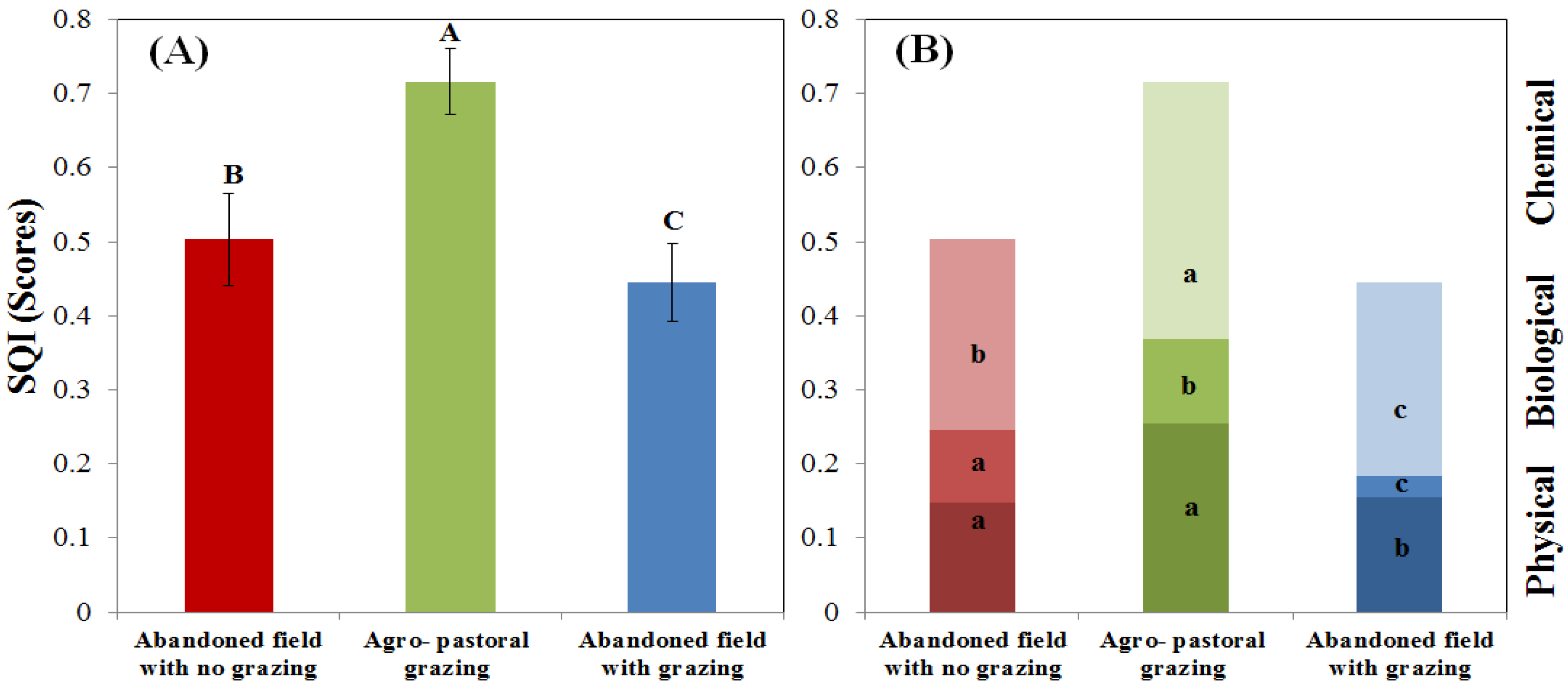
Figure 4.
(A) Scores of soil quality indices (SQIs) for the three land uses in the Migda site, Israel: abandoned field with no grazing (red color), agro-pastoral grazing (green color), and abandoned field with grazing (blue color); and (B) the SQI that was calculated by physical, biological, and chemical analyses. Capital letters above the error bars represent significant differences between land uses. Small letters within the columns represent significant differences between soil components.
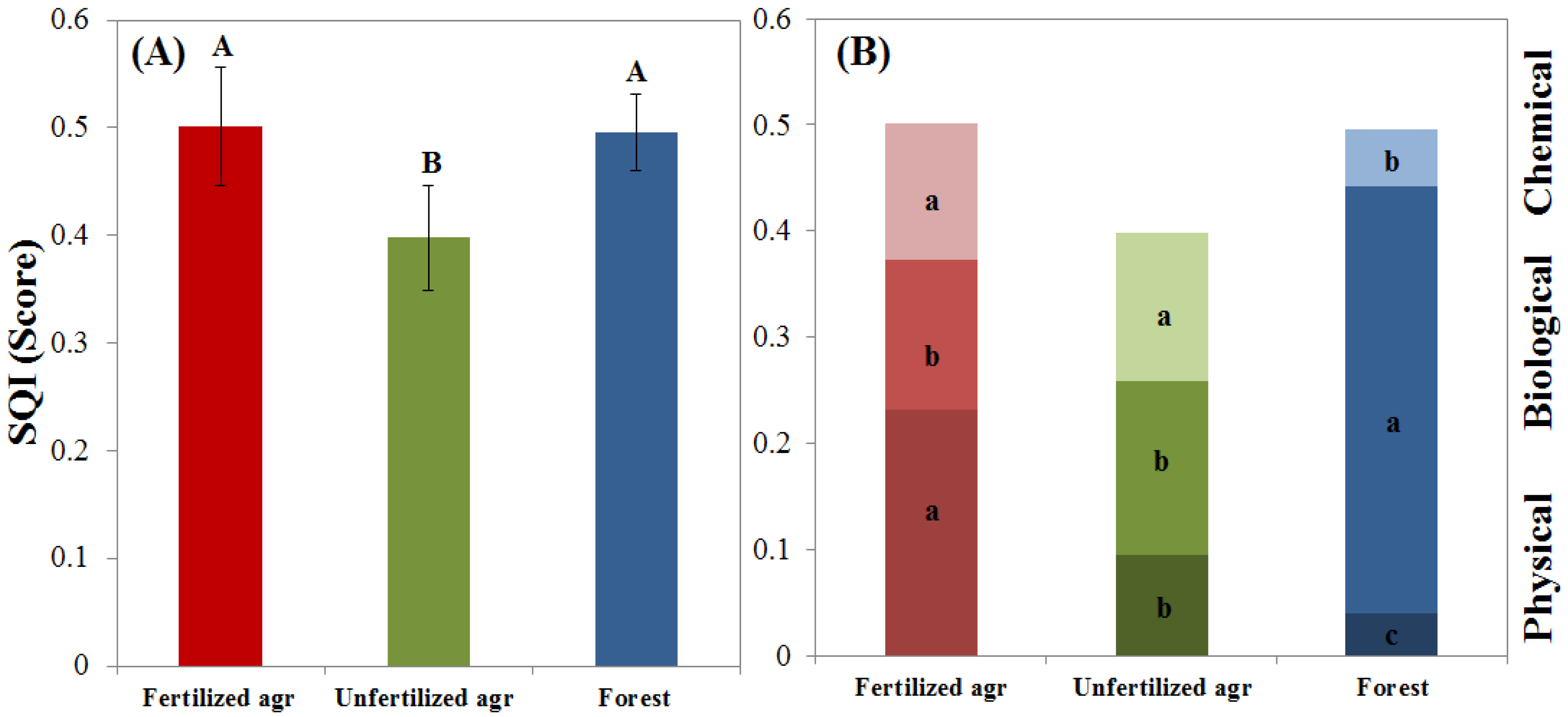
Figure 5.
(A) Scores of soil quality indices (SQIs) for the three land uses in the Schäfertal site, Germany: Fertilize agriculture field (red color), unfertilized agriculture field (green color), and forest (blue color); and (B) the SQI that was calculated by physical, biological, and chemical analyses. Capital letters above the error bars represent significant differences between land uses. Small letters within the columns represent significant differences between soil components.
3.2. Spectral Correlation of Soil Quality Properties
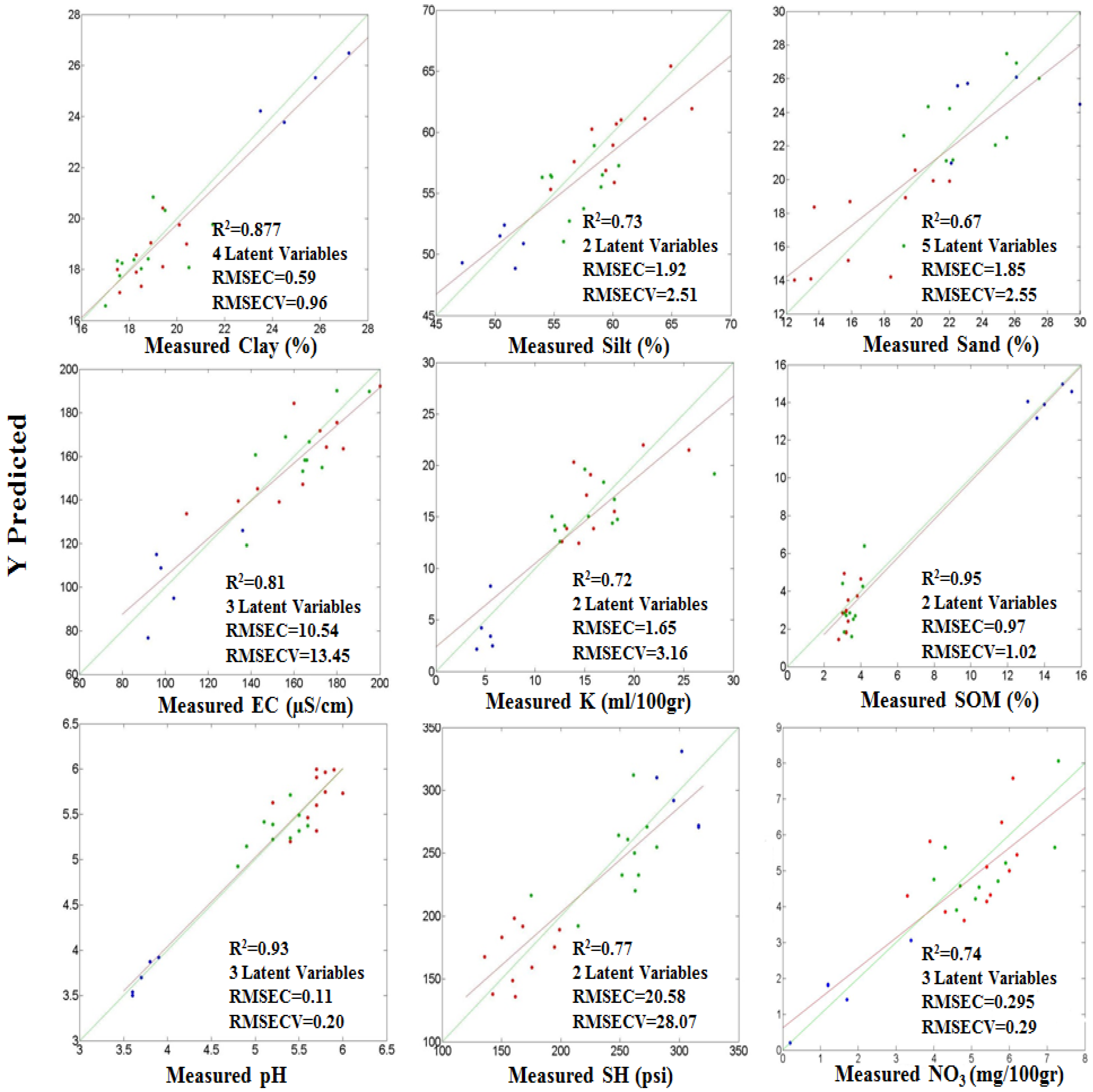
Table 7 presents the results of the PLS-R analysis including the number of latent variables, the coefficient of determination (R
2), the RPD, and the VIP projection. The resultant spectral data that explain a good prediction for the two sites are marked in bold in
Table 7 and in
Figure 6 and
Figure 7. The excellent and good results (“excellent” with RPD ≥ 2.5 and R
2 ≥ 0.80; “good” with RPD between 2–2.5 and R
2 ≥ 0.70) of the PLS-R model prediction in the Migda site include clay, sand and silt content, SH, pH, NH
4, and NO
3. In the Schäfertal site, clay content, SH, SOM, pH, EC, and K showed good results. In addition, the VIP was computed to reveal the score for each wavelength with excellent and good results. The sensitivity bands that were identified by the VIP for the different soil properties and SQI values are presented in
Table 7. These bands are in agreement with those that were previously found in other studies [
14,
31,
70].
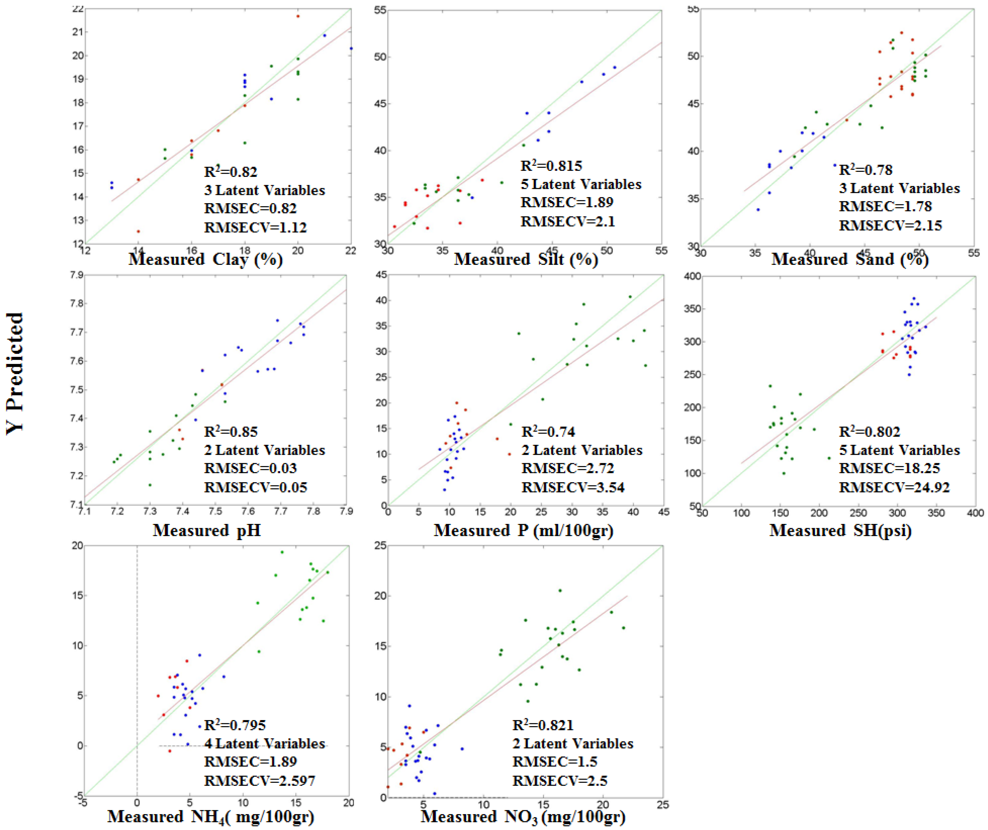
Figure 6 and
Figure 7 shows scatterplots of correlations between soil spectroscopy and laboratory-measured soil values, for the Migda site and Schäfertal site, respectively. The soil properties for the calibration dataset with a coefficient of determination range between 0.67 and 0.95.
Figure 6 and
Figure 7 represents the results by RMSC, RMSCV, R
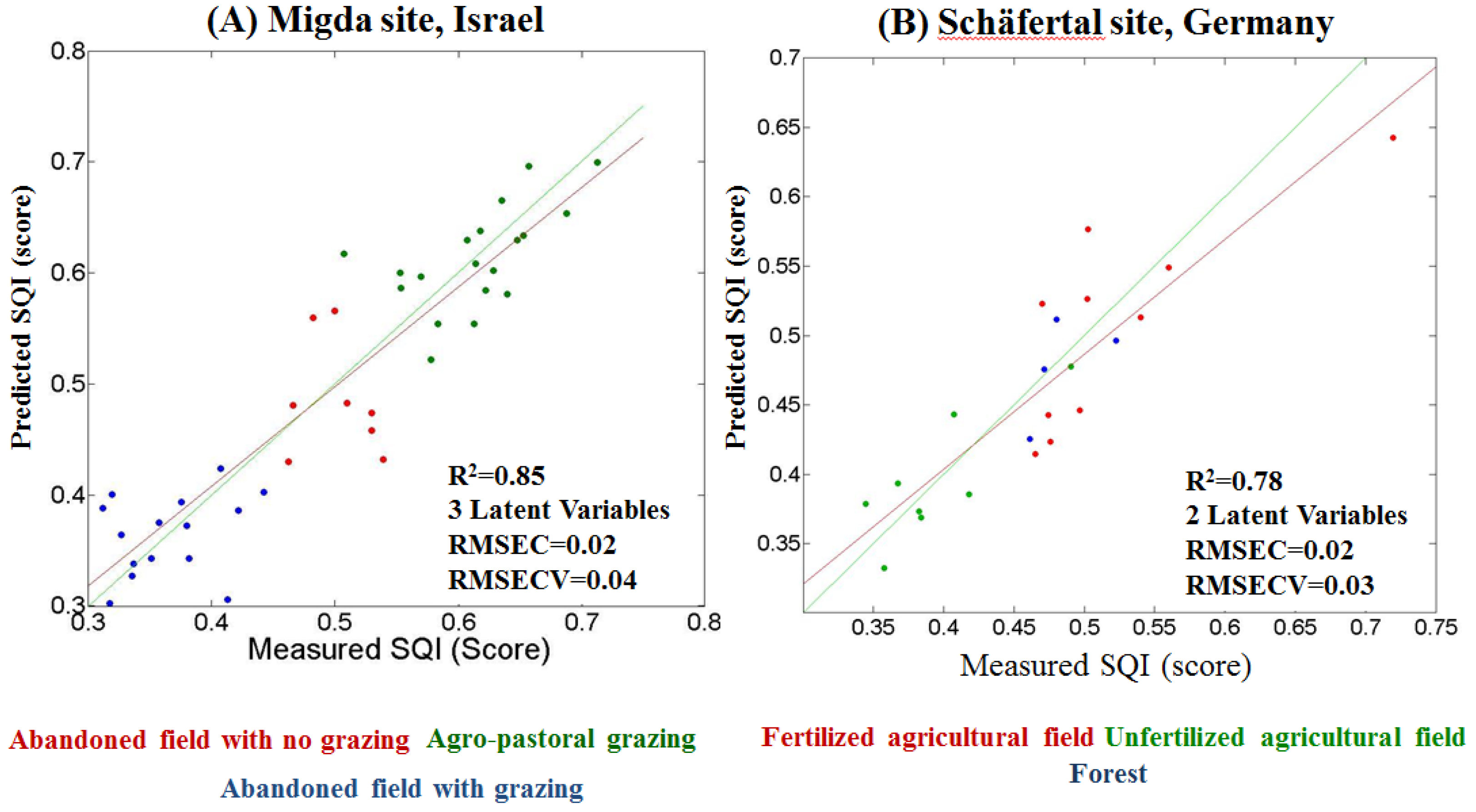
2 and the number of LVs for each soil property as an example. The results of the calculated SQI
versus spectral measurements in the two study sites, along with their RPDs, are presented in
Figure 8. The coefficients of determination in the Migda site were R
2 = 0.84 and RPD = 2.43, and in the Schäfertal site, they were R
2 = 0.78 and RPD = 2.10, both with good prediction accuracy (
Figure 8).
Table 7.
Results of the partial least squares-regression (PLS-R) analysis in terms of spectral regions that are indicative for the soil properties in the two study systems: (1) Migda site, Israel, and (2) Schäfertal site, Germany. Statistics include the number of latent variables (LVs) selected in the PLS-R model, correlation of determination (R2), and the ratio of performance to deviation (RPD). Bold numbers refer to the prediction models that were categorized as “excellent” with RPD ≥ 2.5 and R2 ≥ 0.80, and “good” prediction models with RPD between 2–2.5 and R2 ≥ 0.70. VIP is the variable importance in projection that presents that wavelength (in nanometers) of selected soil properties with excellent and good prediction results.
| Soil properties | Migda Site, Israel | Schäfertal Site, Germany |
|---|
| LVs | R2 | RPD | VIP | LVs | R2 | RPD | VIP |
|---|
| Sand (%) | 3 | 0.78 | 2.19 | 1900; 2220; 2205 | 5 | 0.671 | 1.88 | 1910; 2200; 2300 |
| Silt (%) | 5 | 0.815 | 2.43 | 2 | 0.728 | 1.81 |
| Clay (%) | 3 | 0.827 | 1.81 | 4 | 0.877 | 2.83 |
| AWC (m/m) | 4 | 0.471 | 2.18 | | 4 | 0.739 | 1.72 | |
| SH (psi) | 5 | 0.802 | 2.24 | 1850; 1900; 2140; 2200–2350 | 2 | 0.77 | 2.03 | 1900; 2020 |
| PAC | 4 | 0.677 | 1.84 | | 6 | 0.715 | 1.96 | |
| SOM (%) | 3 | 0.611 | 1.75 | | 2 | 0.951 | 4.16 | 1110; 1170; 1400; 1520; 1900; 2100; 2200 |
| pH | 2 | 0.85 | 3.07 | 517,747,1000; 1400; 1930; 2220 | 3 | 0.93 | 2.65 | 657, 740, 1000; 1400; 1800; 1900; 2200 |
| EC (μS/cm) | 2 | 0.696 | 2.00 | | 3 | 0.809 | 2.38 | 570, 845, 990,1100; 1410; 1850; 1920; |
| N-NH4+ (mg/100gr) | 4 | 0.795 | 2.34 | 590, 870,1850; 2052; 2040 | 2 | 0.267 | 1.69 | |
| N-NO3 (mg/100gr) | 2 | 0.821 | 1.94 | 560, 1770; 1850; 2050 | 3 | 0.741 | 1.76 | |
| K (ml/100gr) | 5 | 0.614 | 2.00 | | 2 | 0.718 | 2.25 | 535, 1500; 1850; 1910; 2020; 2070; 2250 |
| P (mg/100gr) | 2 | 0.74 | 1.92 | | 4 | 0.21 | 0.53 | |
| SQI (overall) | 3 | 0.843 | 2.43 | 570,1200,1780; 1850; 1900; 2100; 2050–2350 | 2 | 0.782 | 2.10 | 560,1100; 1400;1600-1750; 1850; 1900; 2070–2300 |
3.3. Spectral Soil Quality Index (SSQI)
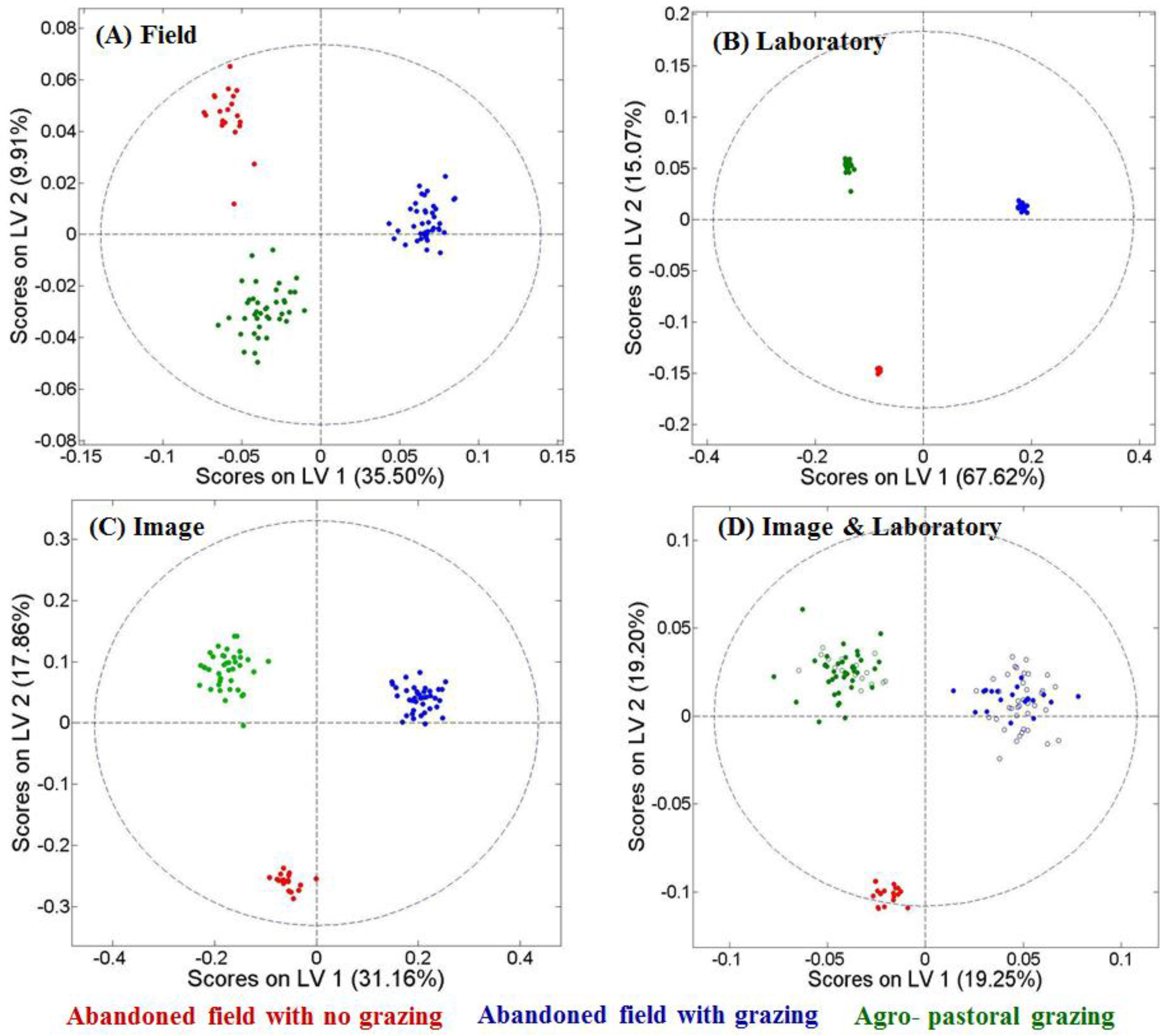
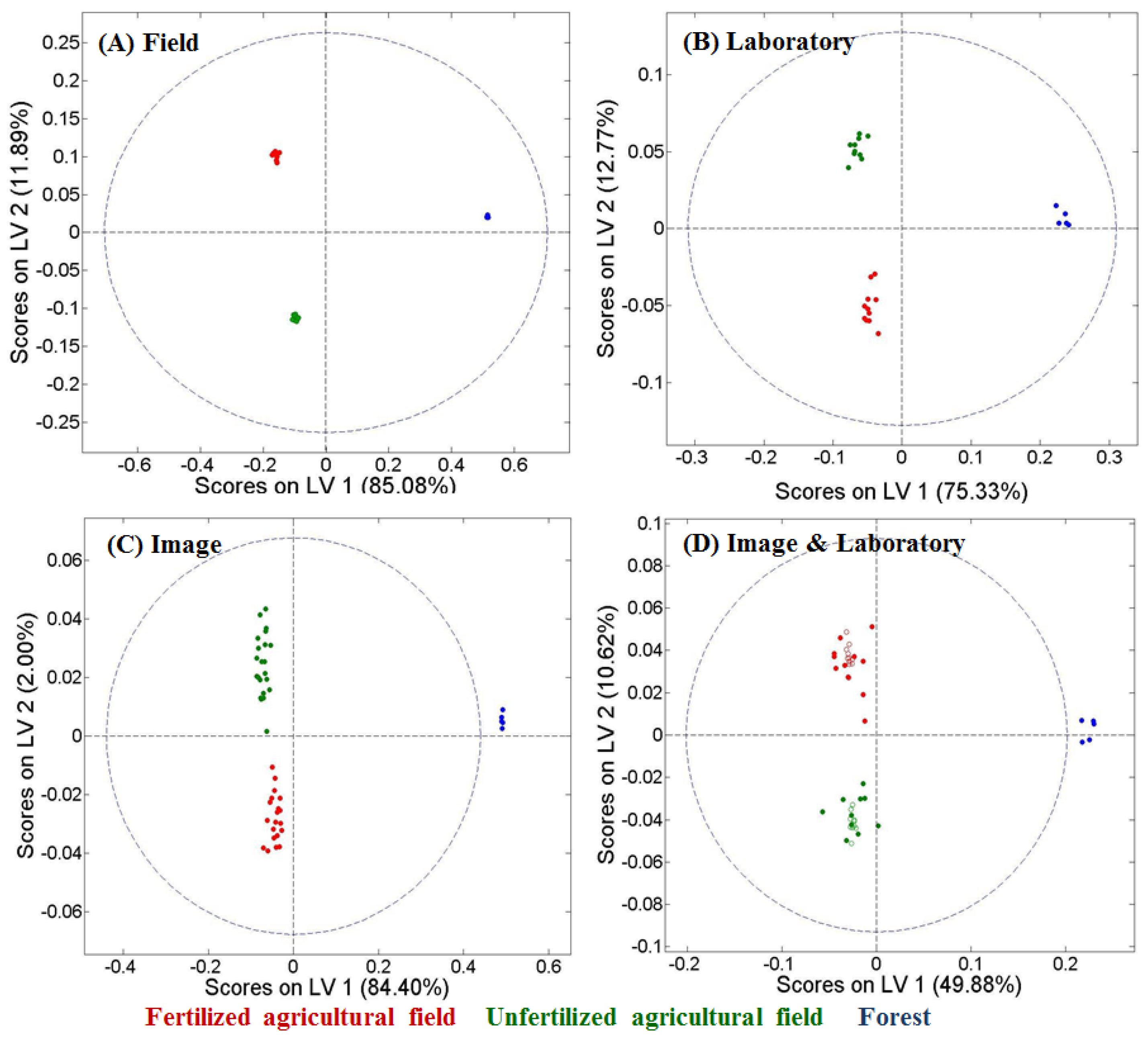
Table 8 shows the total accuracy and the kappa coefficient values of the field and laboratory models, and the prediction model of the whole image in the two sites. The proportional odds in the PLS-DA classification of the spectral samples are presented in
Figure 9 and
Figure 10 for the Migda and the Schäfertal sites, respectively. The results of the classification of the laboratory spectral data had a total accuracy of 1 and a kappa coefficient of 1 in the two sites. The same results were achieved after resampling the data to the AISA sensors (moving from 2000 to either 448 or 366 spectral bands). The results of the classification of the field spectral data had a total accuracy of 0.96 and 0.88, and a kappa coefficient of 0.93 and 0.88 in the Migda and Schäfertal sites, respectively. The results of the classification of the pixels that were extracted from the image showed the same results as the field spectral data, in the two sites. The results of the classification of the combined model (image and laboratory) had a total accuracy of 0.96 and 0.88, and a kappa coefficient of 0.94 and 0.82, in the Migda and Schäfertal sites, respectively. The results of the combined model (image and laboratory) improved the total accuracy. The PLS-DA provides an explicitly quantitative approach to predict the cumulative probability of soil spectral samples that belong to different soil conditions. The results show the ability to classify land uses according to soil function and the effect on the classification accuracy. As expected, moving from laboratory spectroscopy to field spectroscopy and further to IS reduces the classification accuracy.
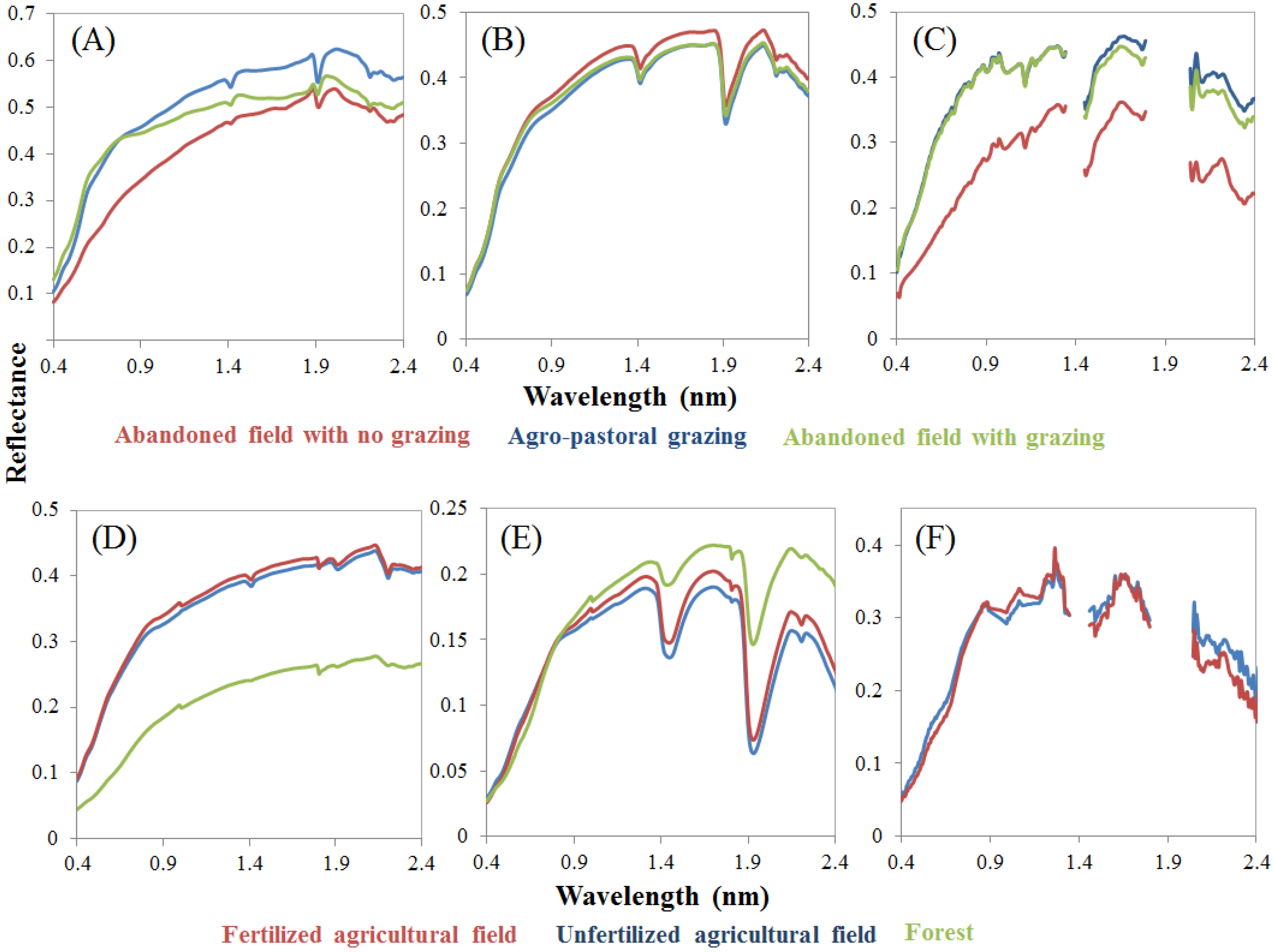
Figure 6.
Scatterplots of cross-validation (CV) predicted values versus measured values for several soil properties for the calibration dataset for all land uses in the Migda site, Israel. Calibration models were developed with a partial least squares-regression (PLS-R). RMSEC: root mean square error of calibration; RMSECV: root mean square error of cross-validation; P: phosphorus p; NH4: ammonium; NH3: nitrate, SH: surface hardness. The colors of the spots represent land-use types: abandoned field with grazing (blue), abandoned field with no grazing (red), agro-pastoral grazing (green).
Figure 7.
Scatterplots of cross-validation (CV) predicted values versus measured values for several soil properties for the calibration dataset for all land uses in the Schäfertal site, Germany. Calibration models were developed with a partial least squares-regression (PLS-R). RMSEC: root mean square error of calibration; RMSECV: root mean square error of cross-validation; EC: electric conductivity; K: potassium; NO3: nitrate; SOM: soil organic matter; SH: surface hardness. The colors of the spots represent land-use types: forest (blue), fertilized agricultural field (red), unfertilized agricultural field (green).
Figure 8.
Scatterplot correlation of soil quality indices (SQI) and reflectance spectroscopy values from the laboratory dataset for the changed land uses: (A) the Migda site, Israel; and (B) the Schäfertal site, Germany. Calibration models were developed with a partial least squares-regression (PLS-R). RMSEC: root mean square error of calibration; RMSECV: root mean square error of cross-validation.
Figure 9.
Partial least squares-discriminant analysis (PLS-DA) classification of the different land uses in the Migda site, Israel, using data of: (A) field spectroscopy; (B) laboratory spectroscopy; (C) airborne imaging spectroscopy; and (D) merged image and laboratory spectroscopy. Dashed circles indicate the 95% confidence level.
Figure 10.
Partial least squares-discriminant analysis (PLS-DA) classification of the different land uses in the Schäfertal site, Germany, using data of: (A) field spectroscopy; (B) laboratory spectroscopy; (C) airborne imaging spectroscopy; and (D) merged image and laboratory spectroscopy. Dashed circles indicate the 95% confidence level.
Table 8.
The results of the classification total accuracy and the kappa coefficient of PLS-DA models as derived for the different land uses of the soil spectral sampling, for the Migda, Israel and Schäfertal, Germany sites.
Table 8.
The results of the classification total accuracy and the kappa coefficient of PLS-DA models as derived for the different land uses of the soil spectral sampling, for the Migda, Israel and Schäfertal, Germany sites.
| Study Site | Spectral Sampling | PLS-DA (Total Accuracy) | PLS-DA (Kappa Coefficient) |
|---|
| Migda, Israel | Laboratory (2000 bands) | 1 | 1 |
| Resampled laboratory (448 bands) | 1 | 1 |
| Field (448 bands) | 0.96 | 0.93 |
| Image (358 bands) | 0.96 | 0.94 |
| Image and laboratory (358 bands) | 0.97 | 0.95 |
| Image prediction (358 bands) | 0.92 | 0.91 |
| Schäfertal, Germany | Laboratory (2000 bands) | 1 | 1 |
| Resampled laboratory (366 bands) | 1 | 1 |
| Field (366 bands) | 0.88 | 0.80 |
| Image (300 bands) | 0.88 | 0.82 |
| Image and laboratory (300 bands) | 0.90 | 0.85 |
| Image prediction (300 bands) | 0.82 | 0.80 |
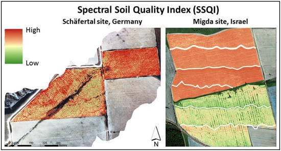
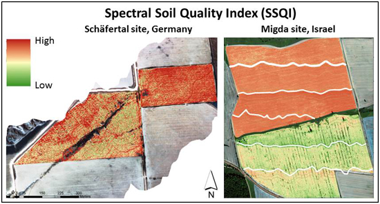
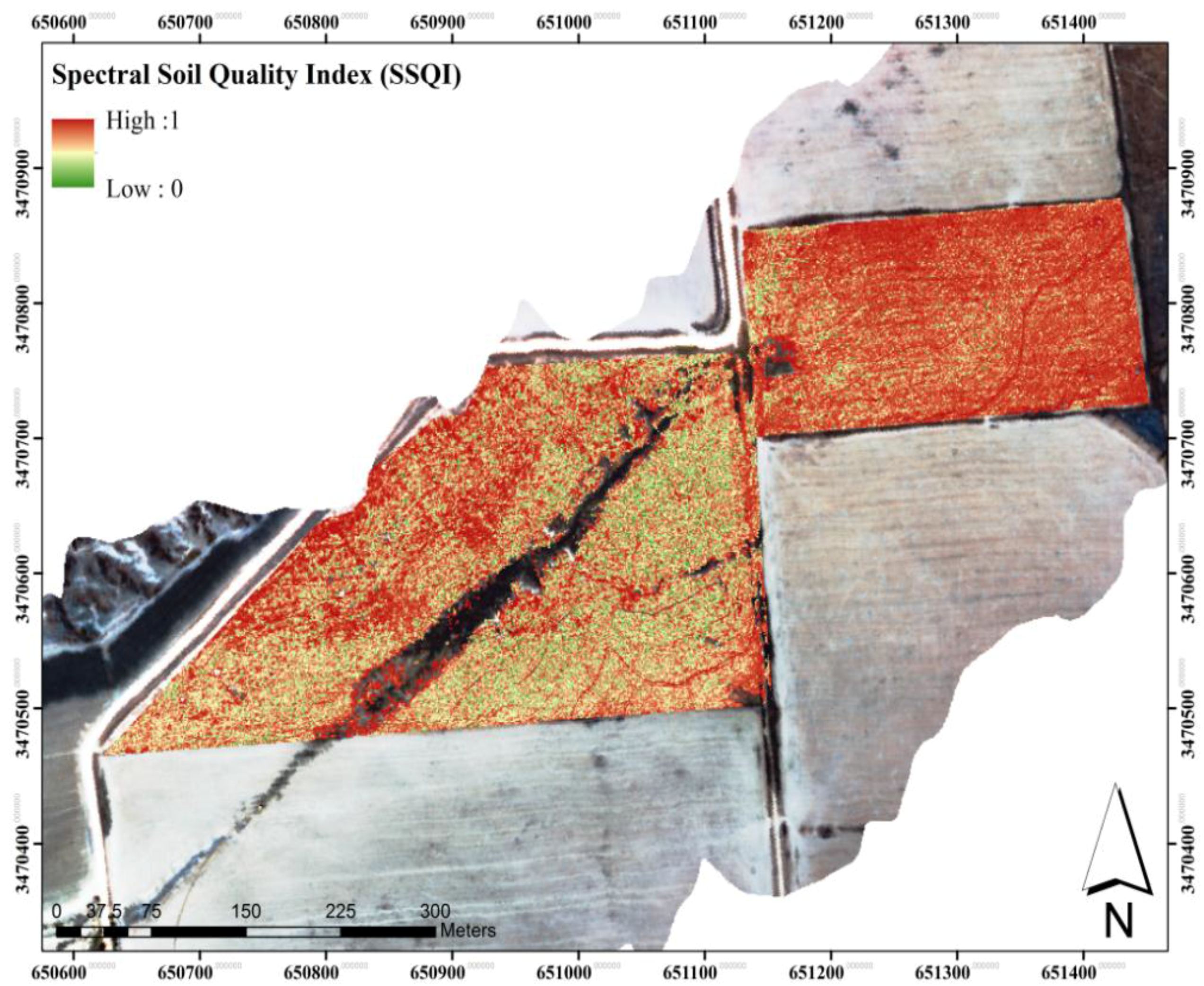
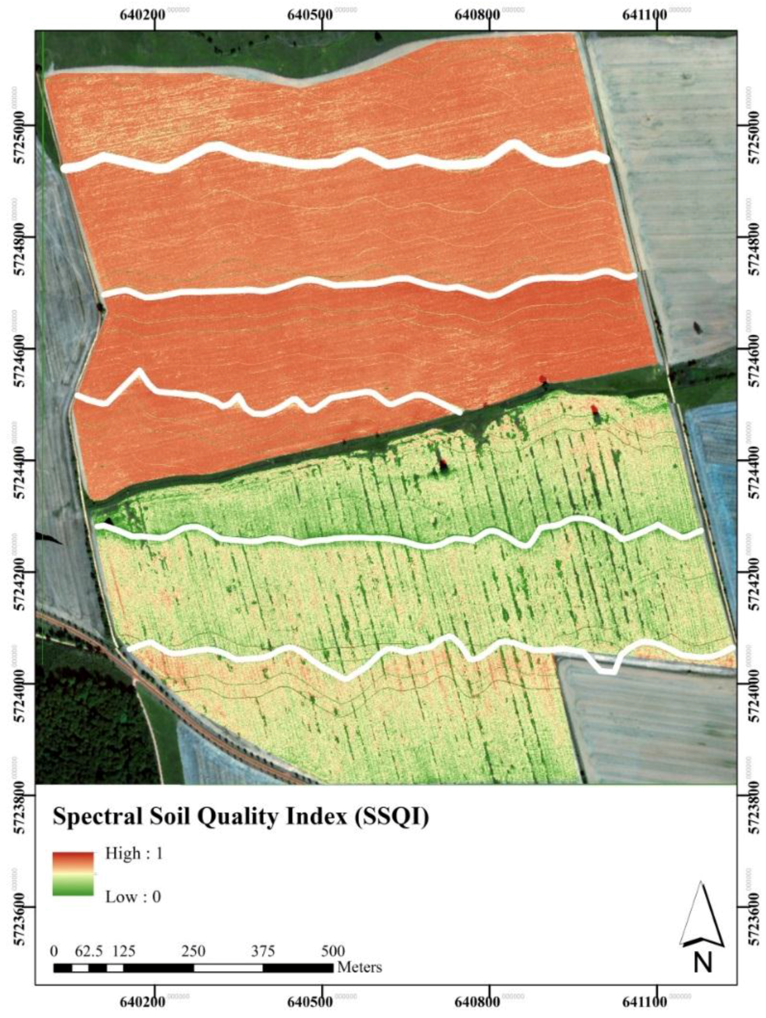
The classifications of the soil condition scores in the two systems were well separated, and each sample represents SSQI scores. The SSQI algorithm was implemented on the output results of the PLS-DA combined model (laboratory spectral data and the extracted pixels from the image). The predictions of the SSQI model in the two sites are shown in
Figure 11 and
Figure 12. The classification predictions of the image had a total accuracy of 0.92 and 0.82, and a kappa coefficient of 0.91 and 0.80, in the Migda and Schäfertal sites, respectively. The SSQI indicates a higher value than the SQI; the model of the SSQI is a proportional model that is not based on the individual probability of each class but on the cumulative probabilities. Therefore, the proportions between classes that explain the changes caused by management are more essential than the actual values. The extracted pixels from the SSQIs predicted from the spectral data were significantly correlated to the SQIs calculated from the laboratory-measured data in the two sites (F = 9.75,
p ≥ 0.01; F = 13.57,
p ≥ 0.01, respectively). The correlations between the SSQI and the SQI were R
2 = 0.71 and R
2 = 0.7, in the Migda and Schäfertal sites, respectively. The spatial selection of the sampling points and the number of sampling affect the strength of the correlation coefficient between the SSQI and SQI.
Figure 11.
Hyperspectral imaging spectroscopy of the spectral soil quality index (SSQI) at Migda site, Israel.
Figure 11.
Hyperspectral imaging spectroscopy of the spectral soil quality index (SSQI) at Migda site, Israel.
Figure 12.
Hyperspectral imaging spectroscopy of the spectral soil quality index (SSQI) at Schäfertal site, Germany.
Figure 12.
Hyperspectral imaging spectroscopy of the spectral soil quality index (SSQI) at Schäfertal site, Germany.


 ,
, 


