
A Hybrid Model for Mapping Relative Differences in Belowground Biomass and Root: Shoot Ratios Using Spectral Reflectance, Foliar N and Plant Biophysical Data within Coastal Marsh


Abstract
:
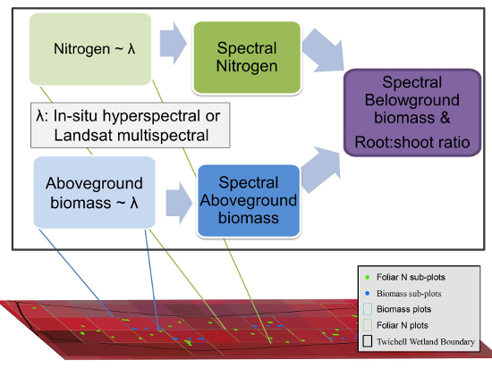
1. Background and Rationale
2. Goals and Objectives
3. Materials and Methods
3.1. Study Area

| Parameter | Twitchell West | Twitchell East | Mayberry |
|---|---|---|---|
| Percent S. acutus | 38 (0–100) | 52 (0–100) | 1 (0–7) |
| Percent Typha spp. | 62 (0–100) | 48 (0–53) | 99 (92–100) |
| S. acutus cover | 12 (0–38) | 18 (0–53) | 1 (0–6) |
| Typha cover | 23 (0–62) | 22 (0–69) | 58 (10–100) |
| Thatch cover | 61 (24–98) | 54 (13–94) | 22 (0–65) |
| Thatch height (cm) | 106 (22–189) | 93 (0–202) | 81 (0–167) |
| Water/Aqu. veg cover | 4 (0–22) | 7 (0–31) | 20 (0–57) |
| Water depth (cm) | 7 (0–30) | 6 (0–38) | 25 (0–66) |

3.2. Data Collection
3.2.1. Measurement of Belowground Biomass
3.2.2. Measurement of Aboveground Biomass
3.2.3. Measurement of Foliar Nitrogen Concentration

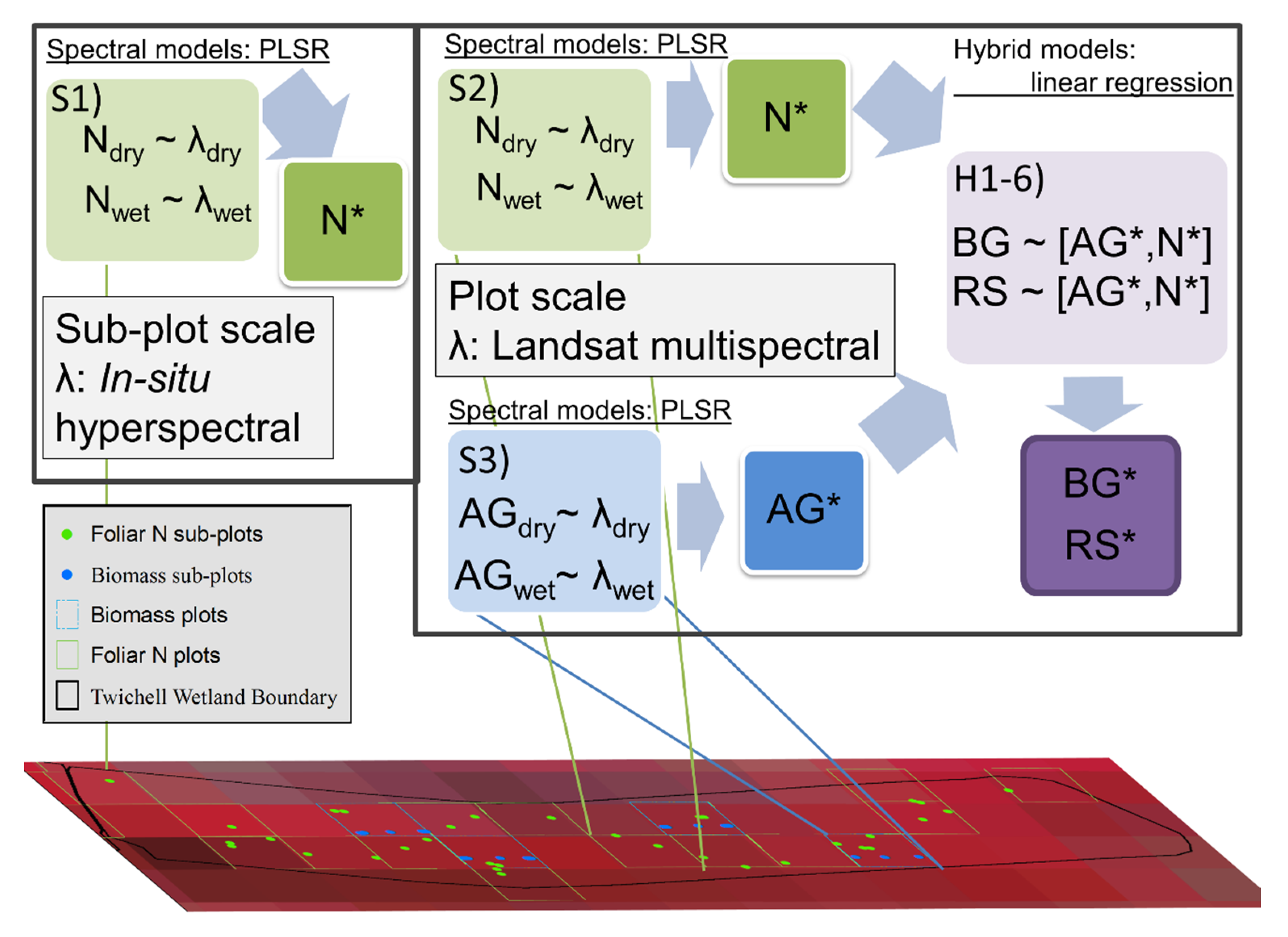
| Model Set | Model Description |
|---|---|
| PLS regression spectral reflectance models | |
| S1 | Predicted % foliar N ~ Hyperspectral reflectance |
| S2 | Predicted % foliar N ~ Multispectral Landsat 7 reflectance |
| S3 | Predicted aboveground biomass ~ Multispectral Landsat 7 reflectance |
| Hybrid models | |
| H1 | Field belowground biomass ~ Predicted N (model S2) |
| H2 | Field belowground biomass ~ Predicted aboveground biomass (model S3 ) |
| H3 | Field belowground biomass ~ Predicted aboveground biomass (model S3) + Predicted N (model S2) |
| H4 | Field root:shoot ratio ~ Predicted N (model S2) |
| H5 | Field root:shoot ratio ~ Predicted aboveground biomass (model S3) |
| H6 | Field root:shoot ratio ~ Predicted belowground biomass (best from models H1-H3)/Predicted aboveground biomass (model S3) |
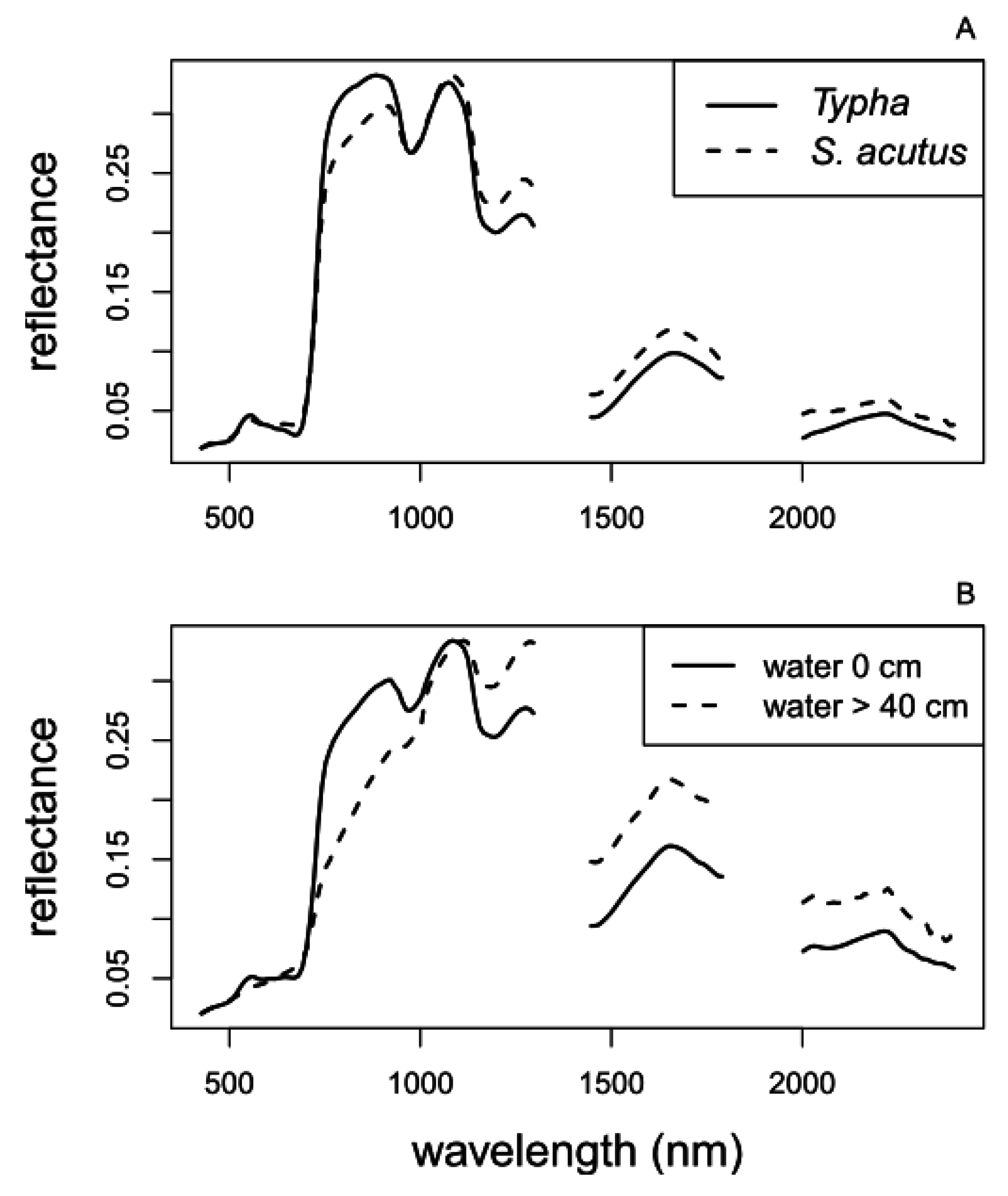
3.2.4. Field Spectroradiometer Reflectance Data Collection
3.2.5. Landsat Image Acquisition and Processing
3.3. Development of Models for Estimating Relative Differences in Belowground Biomass
3.3.1. Remote-Sensing-Based Estimates of Aboveground Biomass and % Foliar N
3.3.2. Hybrid Model Development: Estimating End of Season Belowground Biomass Trends from Remote-Sensing Estimates of Aboveground Biomass and Foliar N
4. Results
| Parameter | Scale | Mean | SD | Min | Max |
|---|---|---|---|---|---|
| S. acutus | |||||
| Belowground biomass | Field: 1 m2 sub-plot | 519 | 571 | 2.5 | 2316 |
| Field: 30 m × 30 m | 270 | 274 | 12.7 | 762 | |
| Landsat: 30 m × 30 m | 395 | 278 | 11 | 691 | |
| Aboveground biomass | Field: 1 m2 sub-plot | 346 | 179 | 72 | 653 |
| Field: 30 m × 30 m | 216 | 123 | 44 | 431 | |
| Landsat: 30 m × 30 m | 308 | 81 | 189 | 442 | |
| Root:shoot ratio | Field: 1 m2 sub-plot | 2.5 | 2.2 | 0.1 | 7.8 |
| Field: 30 m × 30 m | 2.1 | 2.9 | 0.1 | 7.7 | |
| Landsat: 30 m × 30 m | 2.6 | 2.5 | 0.9 | 6.0 | |
| Typha spp. | |||||
| Belowground biomass | Field: 1 m2 sub-plot | 98 | 172 | 1 | 918 |
| Field: 30 m × 30 m | 102 | 88 | 22 | 329 | |
| Landsat: 30 m × 30 m | 102 | 55 | 25 | 166 | |
| Aboveground biomass | Field: 1 m2 sub-plot | 653 | 589 | 20 | 2259 |
| Field: 30 m × 30 m | 625 | 476 | 119 | 1512 | |
| Landsat: 30 m × 30 m | 550 | 386 | 119 | 1061 | |
| Root:shoot ratio | Field: 1 m2 sub-plot | 0.3 | 0.2 | 0.1 | 1.2 |
| Field: 30 m × 30 m | 0.3 | 0.4 | 0.1 | 1.1 | |
| Landsat: 30 m × 30 m | 0.3 | 0.2 | 0.1 | 0.7 | |
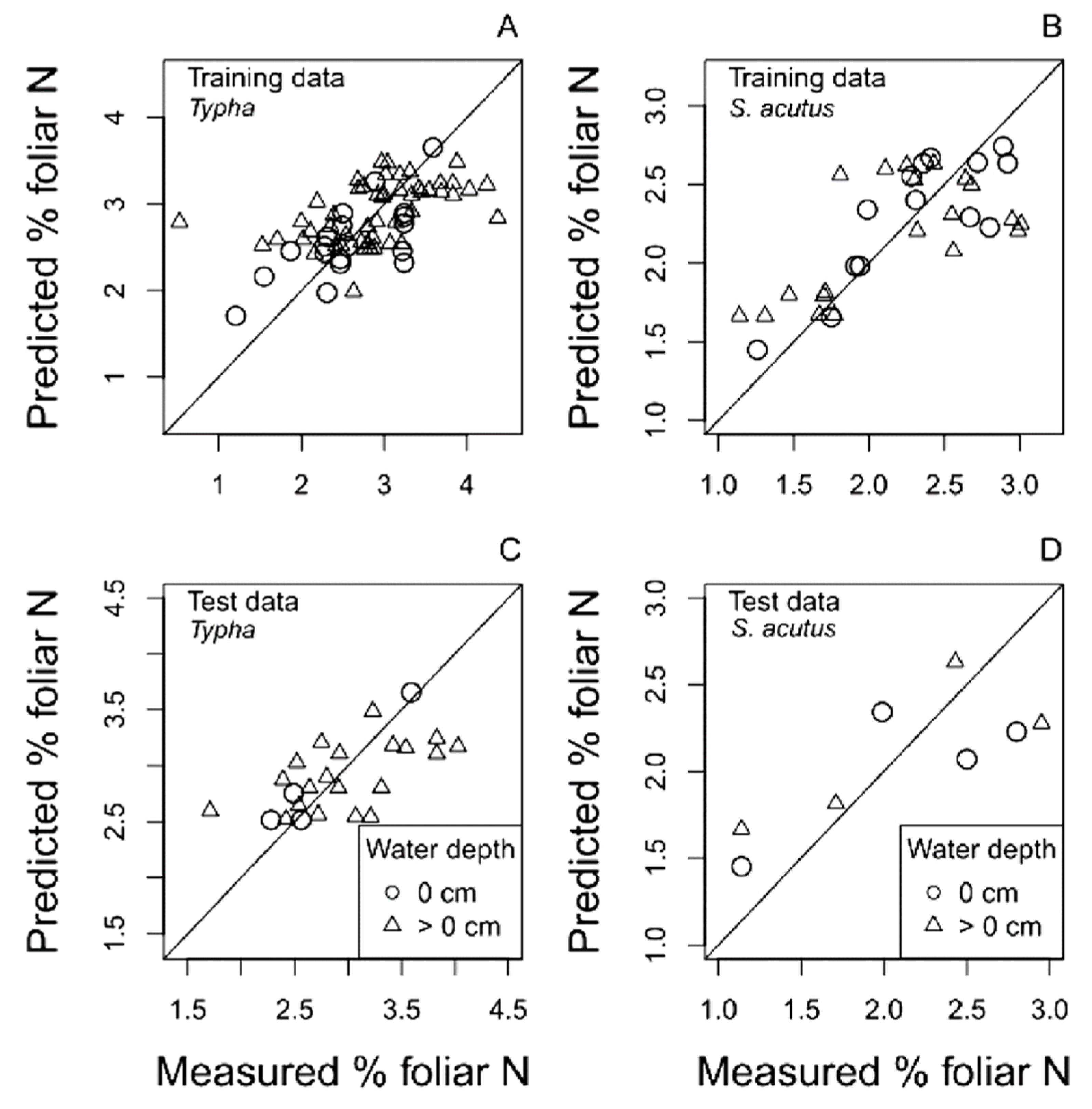
4.1. Foliar N and Aboveground Biomass Spectral Reflectance PLS Regression Models
4.1.1. Hyperspectral Reflectance Models

4.1.2. Multispectral Reflectance Models
| Model | Water depth | Training C. | EV | RMSEP | nRMSEP | N | Testing RMSEP nRMSEP | N | |||
|---|---|---|---|---|---|---|---|---|---|---|---|
| S1a. | % N mixed | = hyperspectral reflectance | 0 | 4 | 54 | 0.46 | 0.20 | 37 | 0.52 | 0.23 | 12 |
| >0 | 14 | 83 | 0.56 | 0.15 | 76 | 0.90 | 0.28 | 28 | |||
| S1b. | % N Typha sp. | = hyperspectral reflectance | 0 | 7 | 90 | 0.50 | 0.24 | 19 | 0.57 | 0.28 | 4 |
| >0 | 6 | 54 | 0.53 | 0.17 | 48 | 0.83 | 0.24 | 18 | |||
| S1c. | % N S. acutus | = hyperspectral reflectance | 0 | 3 | 63 | 0.45 | 0.26 | 15 | 0.43 | 0.33 | 4 |
| >0 | 4 | 62 | 0.47 | 0.23 | 23 | 0.48 | 0.31 | 7 | |||
| S2a. | % N mixed | = Landsat reflectance | 0 | 5 | 56 | 0.49 | 0.25 | 32 | 0.51 | 0.25 | 12 |
| >0 | 3 | 27 | 0.68 | 0.19 | 67 | 0.59 | 0.18 | 25 | |||
| S2b. | % N Typha sp. | = Landsat reflectance | 0 | 3 | 50 | 0.56 | 0.24 | 19 | 0.18 | 0.14 | 4 |
| >0 | 3 | 24 | 0.68 | 0.18 | 50 | 0.83 | 0.21 | 20 | |||
| S2c. | % N S. acutus | = Landsat reflectance | 0 | 3 | 70 | 0.43 | 0.26 | 14 | 0.43 | 0.26 | 4 |
| >0 | 3 | 42 | 0.55 | 0.29 | 20 | 0.44 | 0.24 | 4 | |||
| S3a. | AG mixed | = Landsat reflectance | all | 4 | 53 | 433.3 | 0.14 | 25 | 773.4 | 0.25 | 10 |
| S3a. | AG Typha spp. | = Landsat reflectance | all | 3 | 59 | 448.2 | 0.24 | 21 | 309.3 | 0.25 | 8 |
| S3c. | AG S. acutus | = Landsat reflectance | all | 2 | 67 | 155.5 | 0.20 | 12 | 262.7 | 0.34 | 5 |


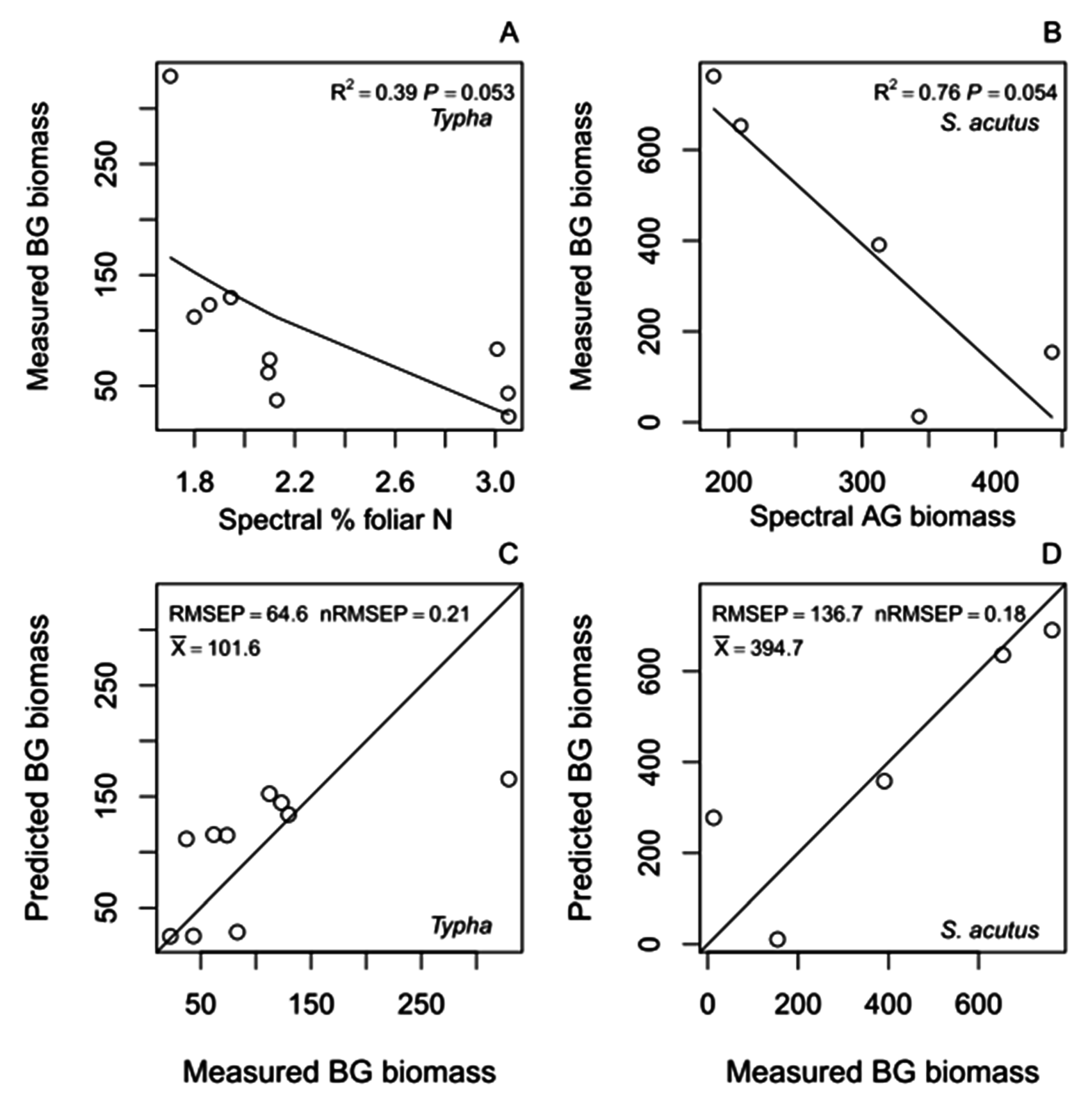
4.2. Predicting Trends in Belowground Biomass and Root:Shoot Ratio Using Satellite-Derived Multispectral Reflectance Hybrid Models
4.2.1. Belowground Biomass Hybrid Models
| Model | Predictors | N | F | df | P | RMSEP | nRMSEP | EV | β0 | L0 | H0 | β1 | L1 | H1 | β2 | L2 | H2 |
|---|---|---|---|---|---|---|---|---|---|---|---|---|---|---|---|---|---|
| Mixed spp. models | |||||||||||||||||
| H1a. BG ~ | log(%N) (S2a) | 12 | 3.4 | 1,10 | 0.094 | 231.1 | 0.29 | 26 | 571 | 282 | 943 | −430 | −904 | −12 | - | - | - |
| H2a. BG ~ | AG (S3a) | 12 | 2.3 | 1,10 | 0.163 | 241.6 | 0.3 | 19 | 1550 | −16 | 3254 | −199 | −446 | 73 | - | - | - |
| H3a. BG ~ | AG (S3a) + log(%N) (S2a) | 12 | 1.6 | 2,9 | 0.248 | 229.3 | 0.29 | 27 | 950 | −807 | 3414 | −69 | −465 | 283 | −342 | −1088 | 327 |
| H4a. RS ~ | log(%N) (S2a) | 12 | 6.9 | 1,10 | 0.026 | 0.4 | 0.27 | 41 | 1.7 | 0.8 | 2.6 | −0.6 | −1.0 | −0.2 | - | - | - |
| H5a. RS ~ | AG (S3a) | 12 | 3.1 | 1,10 | 0.111 | 0.5 | 0.31 | 23 | 1.0 | 0.5 | 1.7 | −0.0 | −0.0 | 0.0 | - | - | - |
| H6a. RS ~ | BG (H1a)/AG (S3a) | 12 | 2.8 | 1,10 | 0.126 | 0.5 | 0.31 | 22 | 0.3 | 0 | 0.8 | 0.3 | 0.1 | 0.8 | - | - | - |
| Typha spp. models | |||||||||||||||||
| H1b. BG ~ | log(%N) (S2b) | 10 | 5.1 | 1,8 | 0.053 | 64.6 | 0.21 | 39 | 294 | 148 | 516 | −242 | −442 | −14 | - | - | - |
| H2b. BG ~ | AG (S3b) | 9 | 2.7 | 1,7 | 0.145 | 71.4 | 0.23 | 28 | 171 | 109 | 308 | −0.1 | −0.2 | 0.1 | - | - | - |
| H3b. BG ~ | AG (S3b) + log(%N) (S2b) | 9 | 5.2 | 2,6 | 0.048 | 50.9 | 0.17 | 64 | 592 | 172 | 958 | 0.4 | −0.1 | 0.9 | −848 | −1698 | −142 |
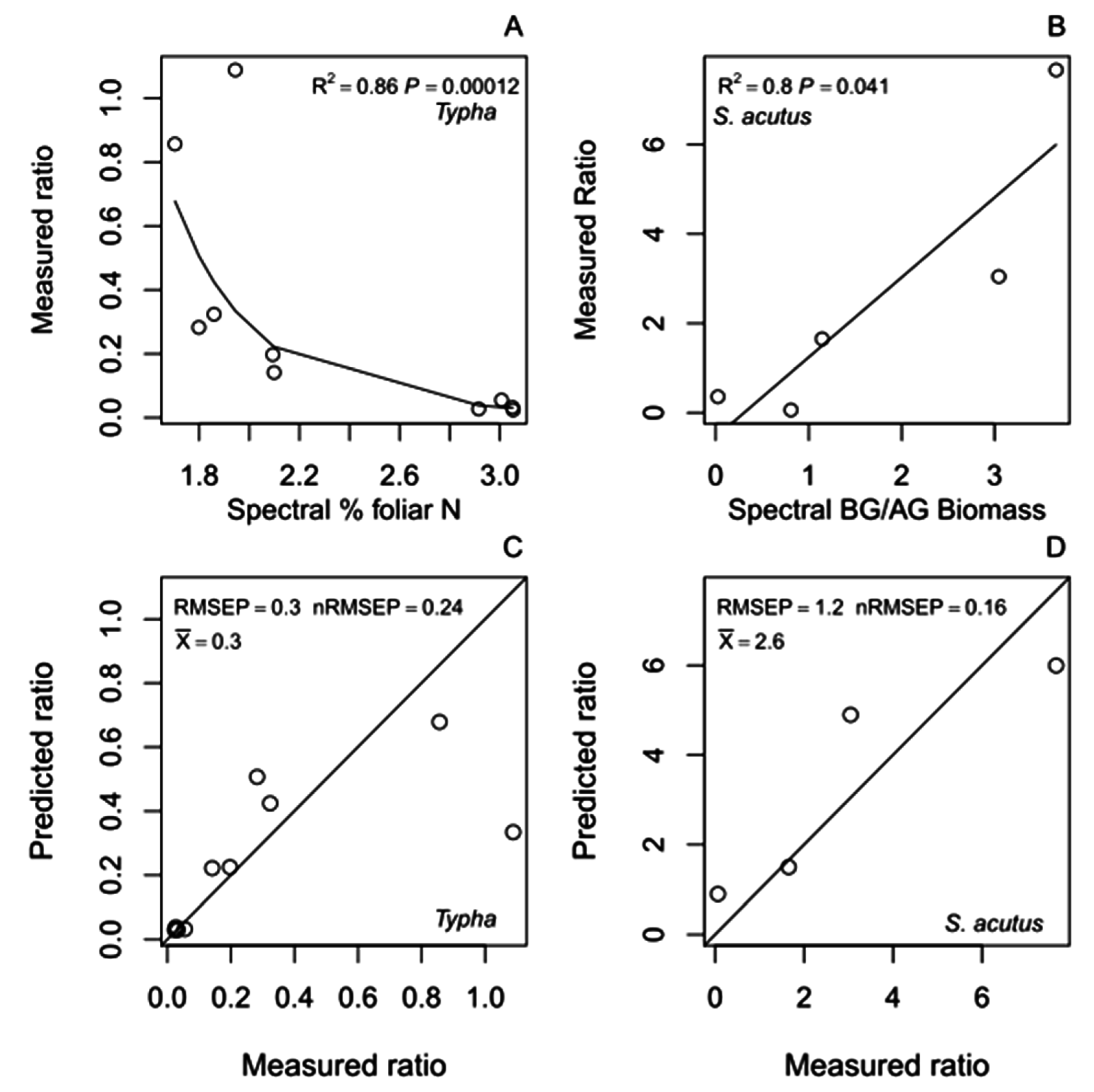
| H4b. RS ~ | log(%N) (S2b) | 10 | 47.7 | 1,8 | <0.001 | 0.3 | 0.24 | 86 | 2.5 | 1.4 | 4.1 | −5.4 | −7.0 | −4.0 | - | - | - |
| H5b. RS ~ | AG (S3b) | 10 | 5.0 | 1,8 | 0.056 | 0.3 | 0.26 | 38 | 0.6 | 0.4 | 1.1 | −0.0 | −0.0 | 0.0 | - | - | - |
| H6b. RS ~ | BG (H1b)/AG (S3b) | 9 | 4.5 | 1,7 | 0.071 | 0.3 | 0.26 | 39 | 0.1 | −0.1 | 0.6 | 0.6 | 0 | 1.2 | - | - | - |
| S. acutus models | |||||||||||||||||
| H1c. BG ~ | log(%N) (S2c) | 8 | 5.9 | 1,6 | 0.052 | 212.6 | 0.29 | 49 | 8 | 6 | 11 | −4 | −9 | −1 | - | - | - |
| H2c. BG ~ | AG (S3c) | 5 | 9.5 | 1,3 | 0.054 | 136.7 | 0.18 | 76 | 1196 | 512 | 1648 | −2 | −5 | −1 | - | - | - |
| H3c. BG ~ | AG (S3c) + log(%N) (S2c) | 5 | 4.5 | 2,2 | 0.181 | 119.3 | 0.16 | 82 | 388 | −2044 | 2237 | −3 | −5 | −1 | 1515 | −2264 | 5282 |
| H4c. RS ~ | log(%N) (S2c) | 5 | 0.5 | 1,3 | 0.537 | 2.5 | 0.33 | 14 | −9.0 | −38.1 | 23.7 | 22.4 | −40.0 | 79.6 | - | - | - |
| H5c. RS ~ | AG (S3c) | 5 | 6.0 | 1,3 | 0.093 | 1.6 | 0.21 | 67 | 9.8 | 4.0 | 16.9 | −0.0 | −0.1 | −0.0 | - | - | - |
| H6c. RS ~ | BG (H2c)/AG (S3c) | 5 | 11.9 | 1,3 | 0.041 | 1.2 | 0.16 | 80 | −0.5 | −2.9 | 1.8 | 1.8 | 0.7 | 2.8 | - | - | - |

4.2.2. Root:Shoot Ratio Hybrid Models

5. Discussion
5.1. Correlations among Foliar N, Aboveground Biomass and Spectral Reflectance
5.2. Estimating Trends in Belowground Biomass and Biomass Allocation Ratio Using Multispectral Hybrid Models
5.3. Applications of Multispectral Hybrid Modeling of Belowground Biomass and Root:Shoot Ratio
6. Conclusions
Acknowledgements
Author Contributions
Conflicts of Interest
Abbreviations Used in Text, Tables and Figures
References
- Smith, M.-L.; Ollinger, S.V.; Martin, M.E.; Aber, J.D.; Hallett, R.A.; Goodale, C.L. Direct estimation of aboveground forest productivity through hyperspectral remote sensing of canopy nitrogen. Ecol. Appl. 2002, 12, 1286–1302. [Google Scholar] [CrossRef]
- Lu, D.S. The potential and challenge of remote sensing-based biomass estimation. Int. J. Remote Sens. 2006, 27, 1297–1328. [Google Scholar] [CrossRef]
- Rasse, D.P.; Rumpel, C.; Dignac, M.-F. Is soil carbon mostly root carbon? Mechanisms for a specific stabilisation. Plant Soil 2005, 269, 341–356. [Google Scholar] [CrossRef]
- Post, W.M.; Emanuel, W.R.; Zinke, P.J.; Stangenberger, A.G. Soil carbon pools and world life zones. Nature 1982, 298, 156–159. [Google Scholar] [CrossRef]
- Moore, P.D. Ecological and hydrological aspects of peat formation. Geol. Soc. Spec. Publ. 1987, 32, 7–15. [Google Scholar] [CrossRef]
- Prokopovich, N.P. Subsidence of peat in California and Florida. Bull. Assoc. Eng. Geol. 1985, 22, 395–420. [Google Scholar] [CrossRef]
- Bridgham, S.D.; Megonigal, J.P.; Keller, J.K.; Bliss, N.B.; Trettin, C. The carbon balance of North American wetlands. Wetlands 2006, 26, 889–916. [Google Scholar] [CrossRef]
- DeLaune, R.D.; Nyman, J.A.; Patrick, W.H., Jr. Peat collapse, ponding and wetland loss in a rapidly submerging coastal marsh. J. Coast. Res. 1994, 10, 1021–1030. [Google Scholar]
- Törnqvist, T.E.; Wallace, D.J.; Storms, J.E.A.; Wallinga, J.; Dam, R.L.; van Blaauw, M.; Derksen, M.S.; Klerks, C.J.W.; Meijneken, C.; Snijders, E.M.A. Mississippi Delta subsidence primarily caused by compaction of Holocene strata. Nat. Geosci. 2008, 1, 173–176. [Google Scholar] [CrossRef]
- Deverel, S.J.; Leighton, D.A. Historic, recent, and future subside, Sacramento-San Joaquin Delta, CA, USA. San Franc. Estuary Watershed Sci. 2010, 8, 1–23. [Google Scholar]
- Nungesser, M.K. Reading the landscape: Temporal and spatial changes in a patterned peatland. Wetlands Ecol. Manag. 2011, 19, 475–493. [Google Scholar] [CrossRef]
- Nyman, J.A.; Delaune, R.D.; Roberts, H.H.; Patrick, W.H. Relationship between vegetation and soil formation in a rapidly submerging coastal marsh. Mar. Ecol. Prog. Ser. 1993, 96, 269–279. [Google Scholar] [CrossRef]
- Morris, J.T.; Sundareshwar, P.V.; Nietch, C.T.; Kjerfve, B.; Cahoon, D.R. Responses of coastal wetlands to rising sea level. Ecology 2002, 83, 2869–2877. [Google Scholar] [CrossRef]
- Miller, R.L.; Fram, M.; Fujii, R.; Wheeler, G. Subsidence reversal in a re-established wetland in the Sacramento-San Joaquin Delta, CA, USA. San Franc. Estuary Watershed Sci. 2008, 6, 1–16. [Google Scholar]
- Zedler, J.B.; Kercher, S. Wetland resources: Status, trends, ecosystem services, and restorability. Annu. Rev. Environ. Resour. 2005, 30, 39–74. [Google Scholar] [CrossRef]
- Benton, A.; Newman, R. Color aerial photography for aquatic plant monitoring. J. Aquat. Plant Manag. 1976, 14, 14–16. [Google Scholar]
- Adam, E.; Mutanga, O.; Rugege, D. Multispectral and hyperspectral remote sensing for identification and mapping of wetland vegetation: A review. Wetlands Ecol. Manag. 2010, 18, 281–296. [Google Scholar] [CrossRef]
- Klemas, V. Remote sensing of coastal wetland biomass: An overview. J. Coast. Res. 2013, 290, 1016–1028. [Google Scholar] [CrossRef]
- Klemas, V. Remote sensing of emergent and submerged wetlands: An overview. Int. J. Remote Sens. 2013, 34, 6286–6320. [Google Scholar] [CrossRef]
- Mishra, D.R.; Cho, H.J.; Ghosh, S.; Fox, A.; Downs, C.; Merani, P.B.T.; Kirui, P.; Jackson, N.; Mishra, S. Post-spill state of the marsh: Remote estimation of the ecological impact of the Gulf of Mexico oil spill on Louisiana Salt Marshes. Remote Sens. Environ. 2012, 118, 176–185. [Google Scholar] [CrossRef]
- Byrd, K.B.; O’Connell, J.L.; Di Tommaso, S.; Kelly, M. Evaluation of sensor types and environmental controls on mapping biomass of coastal marsh emergent vegetation. Remote Sens. Environ. 2014, 149, 166–180. [Google Scholar] [CrossRef]
- Ramsey, E.W., III; Sapkota, S.K.; Barnes, F.G.; Nelson, G.A. Monitoring the recovery of Juncus roemerianus marsh burns with the normalized difference vegetation index and Landsat Thematic Mapper data. Wetlands Ecol. Manag. 2002, 10, 85–96. [Google Scholar] [CrossRef]
- Turpie, K.R.; Klemas, V.V.; Byrd, K.B.; Kelly, M.; Jo, Y.-H. Prospective HyspIRI global observations of tidal wetlands. Remote Sens. Environ. 2015, 167, 206–217. [Google Scholar] [CrossRef]
- Rundquist, D.C.; Narumalani, S.; Narayanan, R.M. A review of wetlands remote sensing and defining new considerations. Remote Sens. Rev. 2001, 20, 207–226. [Google Scholar] [CrossRef]
- Phinn, S.R.; Stow, D.A.; Zedler, J.B. Monitoring wetland habitat restoration in southern California using airborne multi spectral video data. Restor. Ecol. 1996, 4, 412–422. [Google Scholar] [CrossRef]
- Phinn, S.R. A framework for selecting appropriate remotely sensed data dimensions for environmental monitoring and management. Int. J. Remote Sens. 1998, 19, 3457–3463. [Google Scholar] [CrossRef]
- Kearney, M.S.; Stutzer, D.; Turpie, K.; Stevenson, J.C. The effects of tidal inundation on the reflectance characteristics of coastal marsh vegetation. J. Coast. Res. 2009, 256, 1177–1186. [Google Scholar] [CrossRef]
- Turpie, K.R. Explaining the spectral red-edge features of inundated marsh vegetation. J. Coast. Res. 2013, 290, 1111–1117. [Google Scholar] [CrossRef]
- Geladi, P.; Kowalski, B.R. Partial least-squares regression: A tutorial. Anal. Chim. Acta 1986, 185, 1–17. [Google Scholar] [CrossRef]
- Mevik, B.-H.; Cederkvist, H.R. Mean squared error of prediction (MSEP) estimates for principal component regression (PCR) and partial least squares regression (PLSR). J. Chemom. 2004, 18, 422–429. [Google Scholar] [CrossRef]
- Chen, J.; Gu, S.; Shen, M.; Tang, Y.; Matsushita, B. Estimating aboveground biomass of grassland having a high canopy cover: An exploratory analysis of in situ hyperspectral data. Int. J. Remote Sens. 2009, 30, 6497–6517. [Google Scholar] [CrossRef]
- Mokany, K.; Raison, R.J.; Prokushkin, A.S. Critical analysis of root:shoot ratios in terrestrial biomes. Glob. Change Biol. 2006, 12, 84–96. [Google Scholar] [CrossRef]
- Deegan, L.A.; Johnson, D.S.; Warren, R.S.; Peterson, B.J.; Fleeger, J.W.; Fagherazzi, S.; Wollheim, W.M. Coastal eutrophication as a driver of salt marsh loss. Nature 2012, 490, 388–392. [Google Scholar] [CrossRef] [PubMed]
- Yu, Q.; Wu, H.; He, N.; Lü, X.; Wang, Z.; Elser, J.J.; Wu, J.; Han, X. Testing the growth rate hypothesis in vascular plants with above- and below-ground biomass. PLoS ONE 2012, 7, e32162. [Google Scholar] [CrossRef] [PubMed]
- O’Connell, J.L.; Byrd, K.B.; Kelly, M. Remotely-Sensed indicators of N-related biomass allocation in Schoenoplectus acutus. PLoS ONE 2014, 9, e90870. [Google Scholar] [CrossRef] [PubMed]
- Cohen, R.A.; Fong, P. Using opportunistic green macroalgae as indicators of nitrogen supply and sources to estuaries. Ecol. Appl. 2006, 16, 1405–1420. [Google Scholar] [CrossRef]
- Sheppard, J.K.; Carter, A.B.; McKenzie, L.J.; Pitcher, C.R.; Coles, R.G. Spatial patterns of sub-tidal seagrasses and their tissue nutrients in the Torres Strait, northern Australia: Implications for management. Cont. Shelf Res. 2008, 28, 2282–2291. [Google Scholar] [CrossRef]
- Siciliano, D.; Wasson, K.; Potts, D.C.; Olsen, R.C. Evaluating hyperspectral imaging of wetland vegetation as a tool for detecting estuarine nutrient enrichment. Remote Sens. Environ. 2008, 112, 4020–4033. [Google Scholar] [CrossRef] [Green Version]
- Suwandana, E.; Kawamura, K.; Sakuno, Y.; Evri, M.; Lesmana, A.H. Hyperspectral reflectance response of seagrass (Enhalus acoroides) and brown algae (Sargassum sp.) to nutrient enrichment at laboratory scale. J. Coast. Res. 2012, 28, 956–963. [Google Scholar] [CrossRef]
- Mozdzer, T.J.; McGlathery, K.J.; Mills, A.L.; Zieman, J.C. Latitudinal variation in the availability and use of dissolved organic nitrogen in Atlantic coast salt marshes. Ecology 2014, 95, 3293–3303. [Google Scholar] [CrossRef]
- Kobe, R.K.; Iyer, M.; Walters, M.B. Optimal partitioning theory revisited: Nonstructural carbohydrates dominate root mass responses to nitrogen. Ecology 2010, 91, 166–179. [Google Scholar] [CrossRef] [PubMed]
- Mccarthy, M.C.; Enquist, B.J. Consistency between an allometric approach and optimal partitioning theory in global patterns of plant biomass allocation. Funct. Ecol. 2007, 21, 713–720. [Google Scholar] [CrossRef]
- Dong, J.; Kaufmann, R.K.; Myneni, R.B.; Tucker, C.J.; Kauppi, P.E.; Liski, J.; Buermann, W.; Alexeyev, V.; Hughes, M.K. Remote sensing estimates of boreal and temperate forest woody biomass: Carbon pools, sources, and sinks. Remote Sens. Environ. 2003, 84, 393–410. [Google Scholar] [CrossRef]
- Thenkabail, P.S.; Stucky, N.; Griscom, B.W.; Ashton, M.S.; Diels, J.; van der Meer, B.; Enclona, E. Biomass estimations and carbon stock calculations in the oil palm plantations of African derived savannas using IKONOS data. Int. J. Remote Sens. 2004, 25, 5447–5472. [Google Scholar] [CrossRef]
- Townsend, P.A.; Foster, J.R.; Chastain, R.A.; Currie, W.S. Application of imaging spectroscopy to mapping canopy nitrogen in the forests of the central Appalachian Mountains using Hyperion and AVIRIS. IEEE Trans. Geosci. Remote Sens. 2003, 41, 1347–1354. [Google Scholar] [CrossRef]
- Martin, M.E.; Plourde, L.C.; Ollinger, S.V.; Smith, M.-L.; McNeil, B.E. A generalizable method for remote sensing of canopy nitrogen across a wide range of forest ecosystems. Remote Sens. Environ. 2008, 112, 3511–3519. [Google Scholar] [CrossRef]
- Kokaly, R.F.; Asner, G.P.; Ollinger, S.V.; Martin, M.E.; Wessman, C.A. Characterizing canopy biochemistry from imaging spectroscopy and its application to ecosystem studies. Remote Sens. Environ. 2009, 113 (Suppl. S1), S78–S91. [Google Scholar] [CrossRef]
- Liu, J.; Pattey, E.; Miller, J.R.; McNairn, H.; Smith, A.; Hu, B. Estimating crop stresses, aboveground dry biomass and yield of corn using multi-temporal optical data combined with a radiation use efficiency model. Remote Sens. Environ. 2010, 114, 1167–1177. [Google Scholar] [CrossRef]
- Mezzini, E. New Techniques for the Remote Sensing of Foliar Nitrogen Concentration in Forest Ecosystems. Ph.D. Thesis, University of Bologna, Bologna, Italy, 2013. [Google Scholar]
- Phillips, R.L.; Beeri, O.; Liebig, M. Landscape estimation of canopy C:N ratios under variable drought stress in Northern Great Plains rangelands. J. Geophys. Res.-Biogeosci. 2006, 111. [Google Scholar] [CrossRef]
- Zhao, C.J.; Liu, L.Y.; Wang, J.H.; Huang, W.J.; Song, X.Y.; Li, C.J. Predicting grain protein content of winter wheat using remote sensing data based on nitrogen status and water stress. Int. J. Appl. Earth Observ. Geoinf. 2005, 7, 1–9. [Google Scholar] [CrossRef]
- Curran, P.J. Remote sensing of foliar chemistry. Remote Sens. Environ. 1989, 30, 271–278. [Google Scholar] [CrossRef]
- Knyazikhin, Y.; Schull, M.A.; Stenberg, P.; Mõttus, M.; Rautiainen, M.; Yang, Y.; Marshak, A.; Carmona, P.L.; Kaufmann, R.K.; Lewis, P.; et al. Hyperspectral remote sensing of foliar nitrogen content. Proc. Natl. Acad. Sci. USA 2013, 110, E185–E192. [Google Scholar] [CrossRef] [PubMed]
- Stroppiana, D.; Fava, F.; Baschetti, M.; Brivio, P.A. Estimation of nitrogen content in crops and pastures using hyperspectral vegetation indices. In Hyperspectral Remote Sensing of Vegetation; Thenkabail, P.S., Lyon, J.G., Huete, A., Eds.; CRC Press: Boca Raton, FL, USA, 2012; pp. 245–262. [Google Scholar]
- Deverel, S.J.; Rojstaczer, S. Subsidence of agricultural lands in the Sacramento-San Joaquin Delta, California: Role of aqueous and gaseous carbon fluxes. Water Resour. Res. 1996, 32, 2359–2367. [Google Scholar] [CrossRef]
- McKee, K.L. Biophysical controls on accretion and elevation change in Caribbean mangrove ecosystems. Estuar. Coast. Shelf Sci. 2011, 91, 475–483. [Google Scholar] [CrossRef]
- Neill, C. Comparison of soil coring and ingrowth methods for measuring belowground production. Ecology 1992, 73, 1918–1921. [Google Scholar] [CrossRef]
- Hargis, T.G.; Twilley, R.R. Improved coring device for measuring soil bulk density in a Louisiana deltaic marsh. J. Sediment. Res. 1994, 64, 681–683. [Google Scholar] [CrossRef]
- Miller, R.L.; Fujii, R. Plant community, primary productivity, and environmental conditions following wetland re-establishment in the Sacramento-San Joaquin Delta, California. Wetlands Ecol. Manag. 2010, 18, 1–16. [Google Scholar] [CrossRef]
- Masek, J.G.; Vermote, E.F.; Saleous, N.; Wolfe, R.; Hall, F.G.; Huemmrich, F.; Gao, F.; Kutler, J.; Lim, T.K. LEDAPS Landsat Calibration, Reflectance, Atmospheric Correction Preprocessing Code; Oak Ridge National Laboratory Distributed Active: Oak Ridge, TN, USA, 2012; http://0-dx-doi-org.brum.beds.ac.uk/10.3334/ORNLDAAC/1080. [Google Scholar]
- Mevik, B.-H.; Wehrens, R. The PLS package: Principle component and partial least-squares regression in R. J. Stat. Softw. 2007, 18, 1–24. [Google Scholar] [CrossRef]
- Efron, B. Better bootstrap confidence intervals. J. Am. Stat. Assoc. 1987, 82, 171–185. [Google Scholar] [CrossRef]
- Abdel-Rahman, E.M.; Ahmed, F.B.; Ismail, R. Random forest regression and spectral band selection for estimating sugarcane leaf nitrogen concentration using EO-1 Hyperion hyperspectral data. Int. J. Remote Sens. 2013, 34, 712–728. [Google Scholar] [CrossRef]
- Tian, Y.C.; Yao, X.; Yang, J.; Cao, W.X.; Hannaway, D.B.; Zhu, Y. Assessing newly developed and published vegetation indices for estimating rice leaf nitrogen concentration with ground- and space-based hyperspectral reflectance. Field Crops Res. 2011, 120, 299–310. [Google Scholar] [CrossRef]
- Thenkabail, P.S.; Smith, R.B.; De-Pauw, E. Evaluation of narrowband and broadband vegetation indices for determining optimal hyperspectral wavebands for agricultural crop characteristics. Photogramm. Eng. Remote Sens. 2002, 68, 607–621. [Google Scholar]
- Thenkabail, P.S.; Lyon, J.G.; Huete, A. Advances in hyperspectral remote sensing of vegetation and agricultural croplands. In Hyperspectral Remote Sensing of Vegetation; Thenkabail, P.S., Lyon, J.G., Huete, A., Eds.; Taylor and Francis Group: Boca Raton, FL, USA, 2012; pp. 28–29. [Google Scholar]
- Xu, H. Modification of normalised difference water index (NDWI) to enhance open water features in remotely sensed imagery. Int. J. Remote Sens. 2006, 27, 3025–3033. [Google Scholar] [CrossRef]
- Stroppiana, D.; Boschetti, M.; Brivio, P.A.; Bacchi, S. Plant nitrogen concentration in paddy rice from field canopy hyperspectral radiometry. Field Crops Res. 2009, 111, 119–129. [Google Scholar] [CrossRef]
- Ryu, C.; Suguri, M.; Umeda, M. Model for predicting the nitrogen content of rice at panicle initiation stage using data from airborne hyperspectral remote sensing. Biosyst. Eng. 2009, 104, 465–475. [Google Scholar] [CrossRef] [Green Version]
- Mokhele, T.A.; Ahmed, F.B. Estimation of leaf nitrogen and silicon using hyperspectral remote sensing. J. Appl. Remote Sens. 2010, 4, 043560-043560-18. [Google Scholar]
- Sartoris, J.J.; Thullen, J.S.; Barber, L.B.; Salas, D.E. Investigation of nitrogen transformations in a southern California constructed wastewater treatment wetland. Ecol. Eng. 1999, 14, 49–65. [Google Scholar] [CrossRef]
- Bedford, B.L.; Walbridge, M.R.; Aldous, A. Patterns in nutrient availability and plant diversity of temperate North American wetlands. Ecology 1999, 80, 2151–2169. [Google Scholar] [CrossRef]
- Kao, J.T.; Titus, J.E.; Zhu, W.-X. Differential nitrogen and phosphorus retention by five wetland plant species. Wetlands 2003, 23, 979–987. [Google Scholar] [CrossRef]
- Larkin, D.J.; Lishawa, S.C.; Tuchman, N.C. Appropriation of nitrogen by the invasive cattail Typha × glauca. Aquat. Bot. 2012, 100, 62–66. [Google Scholar] [CrossRef]
- Darby, F.A.; Turner, R.E. Below- and aboveground biomass of Spartina alterniflora: Response to nutrient addition in a Louisiana salt marsh. Estuar. Coasts 2008, 31, 326–334. [Google Scholar] [CrossRef]
- Turner, R.E.; Howes, B.L.; Teal, J.M.; Milan, C.S.; Swenson, E.M.; Toner, D.D.G. Salt marshes and eutrophication: An unsustainable outcome. Limnol. Oceanogr. 2009, 54, 1634–1642. [Google Scholar] [CrossRef]
- Morris, J.T.; Shaffer, G.P.; Nyman, J.A. Brinson review: Perspectives on the influence of nutrients on the sustainability of coastal. Wetlands 2013, 33, 975–988. [Google Scholar] [CrossRef]
- Gross, M.F.; Hardisky, M.A.; Wolf, P.L.; Klemas, V. Relationship between aboveground and belowground biomass of Spartina alterniflora (smooth cordgrass). Estuaries 1991, 14, 180–191. [Google Scholar] [CrossRef]
- Valiela, I.; Teal, J.M.; Persson, N.Y. Production and dynamics of experimentally enriched salt marsh vegetation: Belowground biomass. Limnol. Oceanogr. 1976, 21, 245–252. [Google Scholar] [CrossRef]
- Morris, J. A model of growth responses by Spartina alterniflora to nitrogen limitation. J. Ecol. 1982, 70, 25–42. [Google Scholar] [CrossRef]
- Dunbabin, V.; Postma, J.; Schnepf, A.; Pagès, L.; Javaux, M.; Wu, L.; Leitner, D.; Chen, Y.; Rengel, Z.; Diggle, A. Modelling root-soil interactions using three–dimensional models of root growth, architecture and function. Plant Soil 2013, 372, 93–124. [Google Scholar] [CrossRef]
- Morris, J.T. The Marsh Equilibrium Model MEM 3.4. Available online: http://jellyfish.geol.sc.edu/model/marsh/mem.asp (accessed on 3 November 2014).
- Warren Pinnacle Consulting, Inc. SLAMM: Sea Level Affecting Marshes Model. Available online: http://www.warrenpinnacle.com/prof/SLAMM/ (accessed on 4 November 2013).
- Schile, L.M.; Callaway, J.C.; Morris, J.T.; Stralberg, D.; Parker, V.T.; Kelly, M. Modeling tidal marsh distribution with sea-level rise: Evaluating the role of vegetation, sediment, and upland habitat in marsh resiliency. PLoS ONE 2014, 9, e88760. [Google Scholar] [CrossRef] [PubMed]
- Stralberg, D.; Brennan, M.; Callaway, J.C.; Wood, J.K.; Schile, L.M.; Jongsomjit, D.; Kelly, M.; Parker, V.T.; Crooks, S. Evaluating tidal marsh sustainability in the face of sea-level rise: A hybrid modeling approach applied to San Francisco Bay. PLoS ONE 2011, 6, e27388. [Google Scholar] [CrossRef] [PubMed]
- Darby, F.A.; Turner, R.E. Effects of eutrophication on salt marsh root and rhizome biomass accumulation. Mar. Ecol. Prog. Ser. 2008, 363, 63–70. [Google Scholar] [CrossRef]
- Turner, R.E. Wetland loss in the northern Gulf of Mexico: Multiple working hypotheses. Estuaries 1997, 20, 1–13. [Google Scholar] [CrossRef]
- Turner, R.E. Coastal wetland subsidence arising from local hydrologic manipulations. Estuaries 2004, 27, 265–272. [Google Scholar] [CrossRef]
- Day, J.; Britsch, L.; Hawes, S.; Shaffer, G.; Reed, D.; Cahoon, D. Pattern and process of land loss in the Mississippi Delta: A Spatial and temporal analysis of wetland habitat change. Estuar. Coasts 2000, 23, 425–438. [Google Scholar] [CrossRef]
- Weston, N.B. Declining sediments and rising seas: An unfortunate convergence for tidal wetlands. Estuar. Coasts 2014. [Google Scholar] [CrossRef]
- Lane, R.R.; Day, J.W.; Thibodeaux, B. Water quality analysis of a freshwater diversion at Caernarvon, Louisiana. Estuaries 1999, 22, 327–336. [Google Scholar] [CrossRef]
- Wulder, M.A.; Masek, J.G.; Cohen, W.B.; Loveland, T.R.; Woodcock, C.E. Opening the archive: How free data has enabled the science and monitoring promise of Landsat. Remote Sens. Environ. 2012, 122, 2–10. [Google Scholar] [CrossRef]
© 2015 by the authors; licensee MDPI, Basel, Switzerland. This article is an open access article distributed under the terms and conditions of the Creative Commons by Attribution (CC-BY) license (http://creativecommons.org/licenses/by/4.0/).
Share and Cite
O’Connell, J.L.; Byrd, K.B.; Kelly, M. A Hybrid Model for Mapping Relative Differences in Belowground Biomass and Root: Shoot Ratios Using Spectral Reflectance, Foliar N and Plant Biophysical Data within Coastal Marsh. Remote Sens. 2015, 7, 16480-16503. https://0-doi-org.brum.beds.ac.uk/10.3390/rs71215837
O’Connell JL, Byrd KB, Kelly M. A Hybrid Model for Mapping Relative Differences in Belowground Biomass and Root: Shoot Ratios Using Spectral Reflectance, Foliar N and Plant Biophysical Data within Coastal Marsh. Remote Sensing. 2015; 7(12):16480-16503. https://0-doi-org.brum.beds.ac.uk/10.3390/rs71215837
Chicago/Turabian StyleO’Connell, Jessica L., Kristin B. Byrd, and Maggi Kelly. 2015. "A Hybrid Model for Mapping Relative Differences in Belowground Biomass and Root: Shoot Ratios Using Spectral Reflectance, Foliar N and Plant Biophysical Data within Coastal Marsh" Remote Sensing 7, no. 12: 16480-16503. https://0-doi-org.brum.beds.ac.uk/10.3390/rs71215837