Bottom Reflectance in Ocean Color Satellite Remote Sensing for Coral Reef Environments

Abstract

Most ocean color algorithms are designed for optically deep waters, where the seafloor has little or no effect on remote sensing reflectance. This can lead to inaccurate retrievals of inherent optical properties (IOPs) in optically shallow water environments. Here, we investigate in situ hyperspectral bottom reflectance signatures and their separability for coral reef waters, when observed at the spectral resolutions of MODIS and SeaWiFS sensors. We use radiative transfer modeling to calculate the effects of bottom reflectance on the remote sensing reflectance signal, and assess detectability and discrimination of common coral reef bottom classes by clustering modeled remote sensing reflectance signals. We assess 8280 scenarios, including four IOPs, 23 depths and 45 bottom classes at MODIS and SeaWiFS bands. Our results show: (i) no significant contamination (R_rscorr < 0.0005) of bottom reflectance on the spectrally-averaged remote sensing reflectance signal at depths >17 m for MODIS and >19 m for SeaWiFS for the brightest spectral reflectance substrate (light sand) in clear reef waters; and (ii) bottom cover classes can be combined into two distinct groups, “light” and “dark”, based on the modeled surface reflectance signals. This study establishes that it is possible to efficiently improve parameterization of bottom reflectance and water-column IOP retrievals in shallow water ocean color models for coral reef environments.

1. Introduction

Water clarity, or transparency, is an important characteristic of marine ecosystem health, affecting the primary resource (light) required by photosynthetic organisms. Ecosystems such as coral reefs and seagrass meadows are built by photosynthetic organisms, and are therefore highly sensitive to changes in water clarity [1]. Recently, ocean color remote sensing techniques have complemented field sampling to monitor water clarity in coral reefs. Ocean color remote sensing allows large scale, synoptic water clarity monitoring where in situ physical sampling is difficult and costly [2,3]. Satellite sensors provide spectral radiometric measurements of the color of the ocean that can be directly related to the relative concentrations of optically-active constituents, such as phytoplankton, dissolved organic matter or suspended particulate matter [4].

Empirical and physics-based algorithms relate sensor-observed remote-sensing reflectance signals to in situ marine components. The radiative transfer problem of optically deep waters has been widely researched, with deep-water ocean color algorithms meeting NASA mission required accuracies for water-leaving radiance and chlorophyll-a retrievals, e.g., [5,6,7,8]. On the other hand, deriving reliable ocean color products for optically shallow water masses, where light reflected from the seafloor contributes to the net water-leaving radiance, is more challenging and requires specialized algorithms. Water clarity monitoring of optically shallow waters using ocean color imagery data requires an understanding of the effects of bottom reflectance on the surface reflectance signal.

Initial efforts in the development of shallow water inversion algorithms focused primarily on the simultaneous retrieval of bathymetry and bottom cover. Less attention was given to the derivation of the inherent optical properties (IOPs) of the water column [9,10,11,12,13]. More recently, effort has focused on the development of ocean color inversion algorithms for IOP retrievals in optically shallow waters [14,15,16,17]. One example is the newly developed Shallow Water Inversion Model (SWIM) algorithm, currently implemented as an evaluation product in NASA’s ocean color processing code, L2GEN [17]. SWIM is based on the shallow water optical model of Lee et al. [18]; however, the SWIM algorithm does not retrieve water depth and bottom reflectance as free parameters. Instead, estimates of water column depth and benthic albedo (reflectance) are supplied to SWIM as ancillary data inputs. The current implementation of SWIM for the Great Barrier Reef (GBR), Australia, has been developed with the requirement of two specific regional input datasets, bathymetry and benthic albedo: Reliable bathymetry data at 100 m spatial resolution are available over the full extent of the GBR [19]. Prior to this study, an existing benthic biodiversity database [20] was used to derive the bottom reflectance signatures for a simple two-component “light” and “dark” reflectance map [21].

However, the optimal parameterization of bottom reflectance in shallow water inversion models is still not well constrained, particularly with respect to the spectral signature and number of required spectral classes. There remains a need to resolve spectral separability for current ocean color sensors to optimize bottom reflectance parameterization, and thus IOP retrievals in shallow water inversion models.

Quantifying the bottom reflectance contribution to the remote-sensing reflectance signals is challenging due to heterogeneous bottom cover and differences in spatial and spectral resolutions of common ocean color sensors. Current ocean color satellite sensors have limited capabilities to resolve bottom types or communities, such as sand, seagrass, algae or coral, due to the limited number and placement of their spectral bands [22]. Most sensors have 6–15 spectral bands in the 400–1050 nm optical range, spatial pixel resolutions ranging from 250 m to 1.1 km and spatial swath extents of 1000s of kilometers. Whilst planned next generation satellite sensors with improved spectral and/or spatial resolution, such as the Pre-Aerosol Cloud and ocean Ecosystem (PACE) and the Ocean Land Color Instrument (OLCI) (Sentinel-3) missions [23], may be able to better differentiate bottom cover spectral signatures, data acquisition from such sensors is still likely to be coarse, with pixels sizes of 300 m to 1 km in size. Moderate resolution satellite sensors, such as the Moderate Resolution Imaging Spectroradiometer (MODIS), Medium Resolution Imaging Spectrometer (MERIS) and Sea-Viewing Wide Field-of-View Sensor (SeaWiIFS), are currently used by the satellite remote sensing community due to ease of data accessibility and large spatial (global) and temporal (daily) coverage. Numerous previous studies have assessed the spectral separability of different bottom types based on pure endmembers (single organisms or substrate types) within a small area (<1 m²) [24,25,26,27,28,29]. Only a few such investigations, however, have assessed the impact of bottom type mixtures on the remote-sensing reflectance signal [30,31]. Those studies have focused on higher spatial resolution sensors with pixel sizes of <50 m. Data from moderate resolution sensors are represented by 6-to-7 visible bands (Table 1) and relatively large pixel sizes (1 km × 1 km), which typically contain a mixture of bottom types in one pixel. Therefore, it is particularly important to assess the impact of mixed substrate pixels on their spectral separability, rather than analyzing single bottom covers.

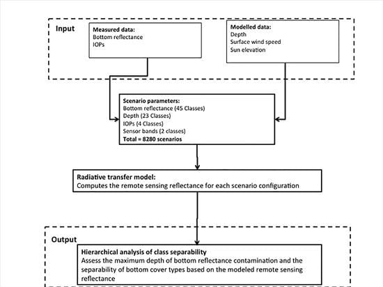
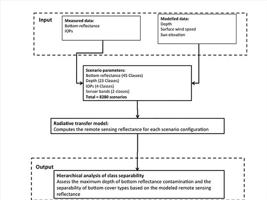
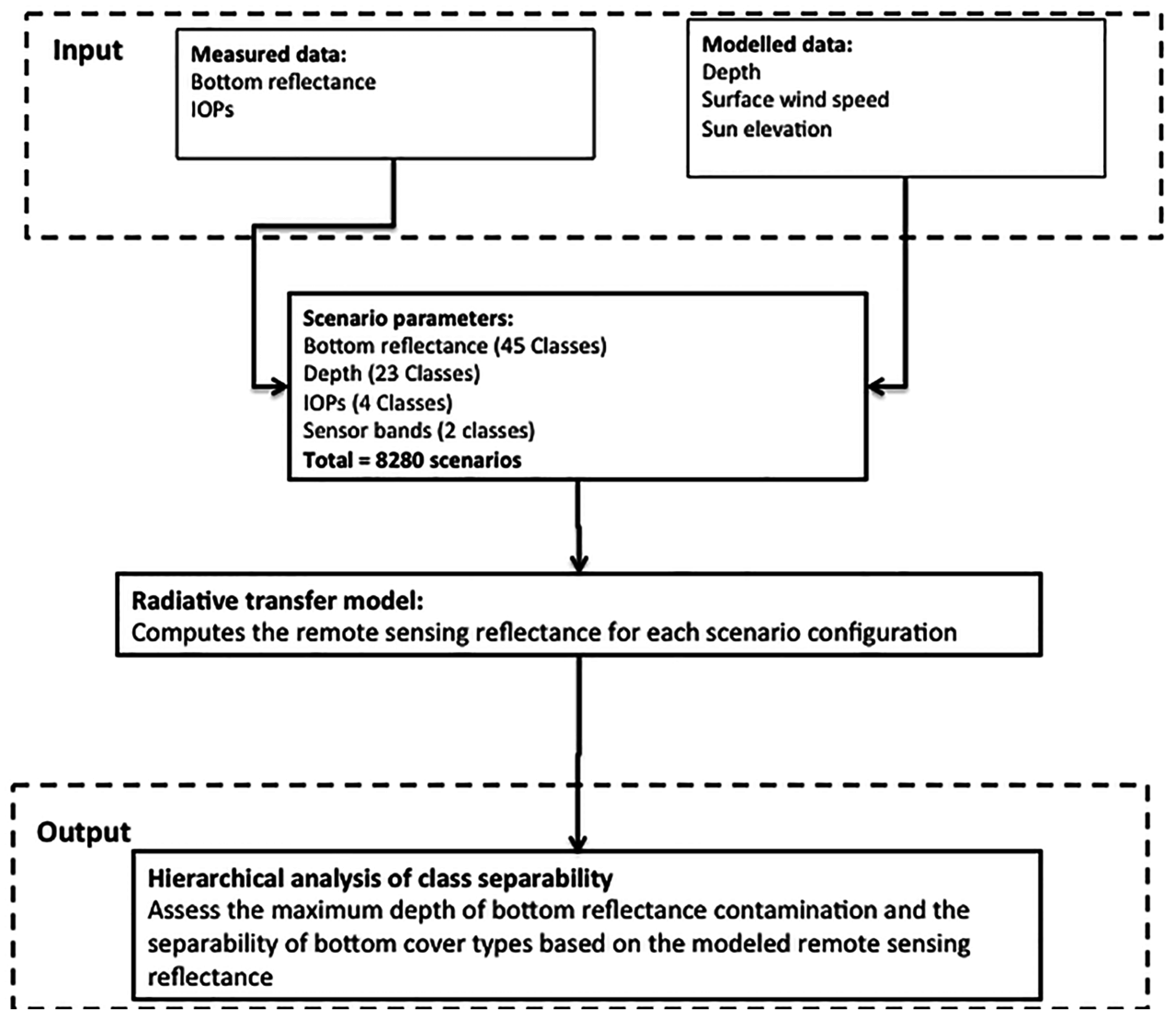
The primary objective of this study therefore was to determine a reliable and efficient approach to discern the optimal bottom cover spectral parameterization for shallow water inversion algorithms. Specifically, we have focused on shallow water inversion algorithms applied to moderate resolution ocean color remote sensing of coral reef environments by: (1) determining threshold depths at which the bottom reflectance signal of individual and mixed bottom types can contribute to the remote-sensing reflectance signal; and (2) determining the number of bottom spectral signatures required to accurately characterize bottom reflectance in shallow water inversion models. We applied the methodology to the MODIS and SeaWiFS spectral bands. Due to project restraints, MERIS data were not used in this study, however the methods are similarly applicable.

Table 1. Assessed band center and bandwidths (nm) used for the statistical analysis of spectral separability and detectability of bottom types.

Sensor	Band Center (Band Width) (units: nm)
MODIS	412.5 (15)	443 (10)	488 (10)	531 (10)	551 (10)	667 (10)	677.5 (10)
SeaWiFS	412 (20)	443 (20)	490 (20)	510 (20)	555 (20)	670 (20)

Table 1. Assessed band center and bandwidths (nm) used for the statistical analysis of spectral separability and detectability of bottom types.

Sensor	Band Center (Band Width) (units: nm)
MODIS	412.5 (15)	443 (10)	488 (10)	531 (10)	551 (10)	667 (10)	677.5 (10)
SeaWiFS	412 (20)	443 (20)	490 (20)	510 (20)	555 (20)	670 (20)

2. Data and Methods

2.1. Methods Overview

Radiative transfer modeling was used to determine the detectability and spectral separability of bottom cover classes through a variety of water column types. The radiative transfer model used, Hydrolight-Ecolight 5 (HE5) [32], was parameterized based on combinations of IOPs, bottom reflectance, depth and sensor type. Output remote-sensing reflectances were then statistically analyzed to determine the detectability and spectral separability of bottom cover classes. The overall modeling approach is illustrated in Figure 1.

Figure 1. Flowchart showing an overview of the input variables for the radiative transfer modeling framework used to conduct a hierarchical analysis of the class spectral separability of common bottom types. The Hydrolight model scenario setup is further described in Table 2.

Figure 1. Flowchart showing an overview of the input variables for the radiative transfer modeling framework used to conduct a hierarchical analysis of the class spectral separability of common bottom types. The Hydrolight model scenario setup is further described in Table 2.

Table 2. Separability scenario description.

Input	Description
Bottom Classes (45 Classes)
Light Sand (carbonate)	Eight endmember (pure bottom) classes were mixed with one another in 25% increments. We then selected 45 classes, eight pure endmember classes and 37 mixed classes. Each class was represented by five spectral reflectance signatures constructed as proportional linear mix from in situ data, except for the coral class, which had ten spectral signatures. A total of 230 bottom scenarios were tested (44 classes * 5 spectral signatures + 10 coral spectral signatures = 230 bottom cover scenarios). Spectra for the scenario classes were derived from existing sources [33,34,35].
Sand (largely terrigenous)
Seagrass
Rock
Rubble
Green Algae
Brown Algae
Live Coral
Depth (23 Classes)
5–49 m	The depth classes were in geometric depth, modeled in 2 m increments.
IOPs (4 Classes)
Reef Waters (Dry Season)	The IOP parameters represent typical optically shallow water environments for the GBR, and were based on field data published in Blondeau-Patissier et al. [36]. As shown in Figure 2 below: “Reef Waters” were located on the outer shelf, within the reef matrix; “Coastal” data were from the inshore Whitsundays region; “Lagoonal” data were from shallow lagoonal stations in the Townsville region with no impact of any estuary or flood plume; “Estuarine” data were collected from the Mossman-Daintree region.
Coastal (Dry Season)
Lagoonal (Dry Season)
Estuarine (Wet Season)
Sensors (2 Classes)
MODIS	The sensors were selected as commonly used in ocean color remote sensing.
SeaWiFS

Table 2. Separability scenario description.

Input	Description
Bottom Classes (45 Classes)
Light Sand (carbonate)	Eight endmember (pure bottom) classes were mixed with one another in 25% increments. We then selected 45 classes, eight pure endmember classes and 37 mixed classes. Each class was represented by five spectral reflectance signatures constructed as proportional linear mix from in situ data, except for the coral class, which had ten spectral signatures. A total of 230 bottom scenarios were tested (44 classes * 5 spectral signatures + 10 coral spectral signatures = 230 bottom cover scenarios). Spectra for the scenario classes were derived from existing sources [33,34,35].
Sand (largely terrigenous)
Seagrass
Rock
Rubble
Green Algae
Brown Algae
Live Coral
Depth (23 Classes)
5–49 m	The depth classes were in geometric depth, modeled in 2 m increments.
IOPs (4 Classes)
Reef Waters (Dry Season)	The IOP parameters represent typical optically shallow water environments for the GBR, and were based on field data published in Blondeau-Patissier et al. [36]. As shown in Figure 2 below: “Reef Waters” were located on the outer shelf, within the reef matrix; “Coastal” data were from the inshore Whitsundays region; “Lagoonal” data were from shallow lagoonal stations in the Townsville region with no impact of any estuary or flood plume; “Estuarine” data were collected from the Mossman-Daintree region.
Coastal (Dry Season)
Lagoonal (Dry Season)
Estuarine (Wet Season)
Sensors (2 Classes)
MODIS	The sensors were selected as commonly used in ocean color remote sensing.
SeaWiFS

The HE5 models spectral remote sensing reflectance (R_rs) based on user-specified geometric depth, spectral values of water-column IOPs, and bottom reflectance. Here, HE5 was configured to calculate R_rs for the spectral bands of the SeaWiFS and MODIS sensors. We used built-in HE5 sensor spectral bands for MODIS and SeaWiFS, which include the sensor bands as well as some intermediate bands. For the statistical analysis of bottom type spectral separability and detectability, we only used the spectral bands listed in Table 1.

The R_rs values were calculated for each bottom class (i), IOP configuration (w) and specific sensor bands (W) at incremental depths (z) from 5 m to 49 m (see Table 2). A baseline model, where the bottom reflectance was set to zero (black/non-reflective), was used to calculate the water column contribution to the R_rs for each IOP, depth increment and sensor band combination.

Our study excluded depths shallower than 5 m, where benthic reflectance is likely to dominate the surface reflectance signal potentially causing sensor saturation. In these very shallow waters (<5 m), IOP retrievals are expected to be unreliable because the water column optical interactions contribute less to the remote-sensing reflectance than bottom reflectance. The deepest depth modeled, 49 m, was expected to be deep enough such that there would be no benthic reflectance contribution the water-leaving signal.

To parameterize the spectral shape and magnitude of IOPs used in the HE5 simulations, the concentration of constituent matter (Chl and total suspended solids) and the spectral slope of the colored dissolved organic matter absorption coefficient were required. For this study, typical values for the four optical classed were based on in situ measurements in GBR waters, as reported by Blondeau-Patissier et al. [36], with locations shown in Figure 2. Table 3 provides a summary of the constituent concentrations representative of the four optical scenarios used in our study. The built-in MODIS and SeaWiFS bands in HE5 were used to simulate the spectral R_rs signals for each scenario.

Figure 2. Map showing sampling locations for the four inherent optical property scenarios used: Coastal, Estuarine, Lagoonal and Reef Waters of the Great Barrier Reef (adapted from Blondeau-Patissier et al. [36]).

Figure 2. Map showing sampling locations for the four inherent optical property scenarios used: Coastal, Estuarine, Lagoonal and Reef Waters of the Great Barrier Reef (adapted from Blondeau-Patissier et al. [36]).

Table 3. Optically active constituent matter values used in Hydrolight 5 to calculate inherent optical properties. Values are from Blondeau-Patissier et al. [36].

Parameter	Abbreviation	Units	Estuarine	Lagoonal	Coastal	Reef
Chlorophyll concentration	Chl	mg·m−3	3.165	0.441	0.7605	0.1345
Total Suspended Solids concentration	TSS	mg·L−1	11.63	3.65	6.35	1.4
Colored Dissolved Organic Matter Spectral Slope	SCDOM	nm−1	0.016	0.0215	0.0185	0.0145

Table 3. Optically active constituent matter values used in Hydrolight 5 to calculate inherent optical properties. Values are from Blondeau-Patissier et al. [36].

Parameter	Abbreviation	Units	Estuarine	Lagoonal	Coastal	Reef
Chlorophyll concentration	Chl	mg·m−3	3.165	0.441	0.7605	0.1345
Total Suspended Solids concentration	TSS	mg·L−1	11.63	3.65	6.35	1.4
Colored Dissolved Organic Matter Spectral Slope	SCDOM	nm−1	0.016	0.0215	0.0185	0.0145

2.2. Bottom Reflectance Dataset

Our study used published datasets of in situ spectral reflectance signatures for selected biotic and abiotic coral reef features and communities from various global locations representative of coral reef environments. These environments included the GBR, Australia, Fiji, the Cook Islands and Belize [33,34,35]. The datasets comprised reflectance spectra of different bottom types obtained in situ, using a spectrometer in a custom-made underwater housing. All the bottom cover spectra were considered also representative of bottom cover classes occurring in the GBR. Eight endmember classes were selected: light sand (carbonate), darker (largely terrigenous) sand, rock, rubble, live coral, green algae, brown algae, and seagrass. These endmember classes were selected based on their frequency of occurrence in the GBR, and their potential spectral separability based on previous research [25,30,31,37,38,39,40]. The eight classes were then linearly mixed by percentage with each other in 25%:75%, 50%:50% and 75%:25% proportions, to provide a total of 84 mixed classes. The mixed bottom classes were calculated using two different bottom classes only.

The following linear mixing method was applied:

$$M_i={\displaystyle \sum _{\mathrm{j}=1}^{\mathrm{n}}}({\mathrm{R}}_{\text{ij}}\cdot {\mathrm{F}}_{\mathrm{j}})$$

(1)

where i = 1, …, m represents the number of bands, j = 1, …, n is number of endmembers (for our study n = 2), M_i is the spectral reflectance of the i^th spectral band of a spectral mixture, R_ij is the spectral reflectance of the j^th component and F_j is the fraction coefficient of the j^th component.

A selection (47) of mixed bottom classes were then subjectively eliminated from further consideration because they are less common in shallow coral reef environments. For example, seagrass does not grow on coral or rock, and light sand does not generally occur in the same pixel as terrigenous sand. A total of 37 remaining mixed bottom classes were used in this study. Table 4 shows the assessed bottom classes, comprising eight endmember and 37 mixed classes, as well as mixed classes excluded from the study.

Table 4. Assessed endmember and mixed bottom classes, and excluded mixed bottom classes.

Assessed Endmembers (8 Classes)
Coral (100)	Light sand (100)
Green algae (100)	Rock (100)
Brown algae (100)	Rubble (100)
Seagrass (100)	Sand (100)
Assessed Mixed Bottom Classes (37 Classes)
Brown algae: Green algae (50:50, 25:75)	Sand: Coral (75:25)
Brown algae: Coral (50:50, 75:25)	Sand: Rock (50:50, 75:25)
Green algae: Coral (75:25)	Sand: Rubble (50:50, 75:25)
Light sand: Brown algae (50: 50, 75:25)	Sand: Brown algae (50:50, 75:25)
Light sand: Green algae (50: 50, 75:25)	Sand: Green algae (50:50, 75:25)
Light sand: Rock (50:50, 75:25)	Sand: Seagrass (50:50, 75:25)
Light sand: Rubble (50:50, 75:25)	Seagrass: Rubble (50:50, 75:25)
Light sand: Seagrass (50:50, 75:25)	Seagrass: Brown algae (75:25)
Light sand: Coral (75:25)	Seagrass: Green algae (75:25)
Rubble: Brown algae (50:50, 75:25)	Seagrass: Rock (75:25)
Rubble: Green algae (50:50, 75:25)
Rubble: Coral (75:25)
Excluded Bottom Classes (47)
Brown algae: Green algae (25:75)	Rubble: Rock (50:50, 75:25, 25:75)
Brown algae: Coral (25:75)	Rock: Coral (50:50, 75:25, 25:75)
Coral: Seagrass (50:50, 75:25, 25:75)	Rock: Brown algae (50:50, 75:25, 25:75)
Green algae: Coral (50:50, 25:75)	Rock: Green algae (50:50, 75:25 , 25:75)
Light sand: Coral (50:50, 25:75)	Sand: Coral (50:50, 25:75)
Light sand: Brown algae (25:75)	Sand: Brown algae (25:75)
Light sand: Green algae (25:75)	Sand: Green algae (25:75)
Light sand: Rock (25:75)	Sand: Rock (25:75)
Light sand: Rubble (25:75)	Sand: Rubble (25:75)
Light sand: Seagrass (25:75)	Sand: Seagrass (25:75)
Light sand: Sand (50:50, 75:25, 25:75)	Seagrass: Rubble (25:75)
Rubble: Brown algae (25:75)	Seagrass: Brown algae (50:50, 25:75)
Rubble: Green algae (25:75)	Seagrass: Green algae (50:50, 25:75)
Rubble: Coral (50:50, 25:75)	Seagrass: Rock (50:50, 25:75)

Table 4. Assessed endmember and mixed bottom classes, and excluded mixed bottom classes.

Assessed Endmembers (8 Classes)
Coral (100)	Light sand (100)
Green algae (100)	Rock (100)
Brown algae (100)	Rubble (100)
Seagrass (100)	Sand (100)
Assessed Mixed Bottom Classes (37 Classes)
Brown algae: Green algae (50:50, 25:75)	Sand: Coral (75:25)
Brown algae: Coral (50:50, 75:25)	Sand: Rock (50:50, 75:25)
Green algae: Coral (75:25)	Sand: Rubble (50:50, 75:25)
Light sand: Brown algae (50: 50, 75:25)	Sand: Brown algae (50:50, 75:25)
Light sand: Green algae (50: 50, 75:25)	Sand: Green algae (50:50, 75:25)
Light sand: Rock (50:50, 75:25)	Sand: Seagrass (50:50, 75:25)
Light sand: Rubble (50:50, 75:25)	Seagrass: Rubble (50:50, 75:25)
Light sand: Seagrass (50:50, 75:25)	Seagrass: Brown algae (75:25)
Light sand: Coral (75:25)	Seagrass: Green algae (75:25)
Rubble: Brown algae (50:50, 75:25)	Seagrass: Rock (75:25)
Rubble: Green algae (50:50, 75:25)
Rubble: Coral (75:25)
Excluded Bottom Classes (47)
Brown algae: Green algae (25:75)	Rubble: Rock (50:50, 75:25, 25:75)
Brown algae: Coral (25:75)	Rock: Coral (50:50, 75:25, 25:75)
Coral: Seagrass (50:50, 75:25, 25:75)	Rock: Brown algae (50:50, 75:25, 25:75)
Green algae: Coral (50:50, 25:75)	Rock: Green algae (50:50, 75:25 , 25:75)
Light sand: Coral (50:50, 25:75)	Sand: Coral (50:50, 25:75)
Light sand: Brown algae (25:75)	Sand: Brown algae (25:75)
Light sand: Green algae (25:75)	Sand: Green algae (25:75)
Light sand: Rock (25:75)	Sand: Rock (25:75)
Light sand: Rubble (25:75)	Sand: Rubble (25:75)
Light sand: Seagrass (25:75)	Sand: Seagrass (25:75)
Light sand: Sand (50:50, 75:25, 25:75)	Seagrass: Rubble (25:75)
Rubble: Brown algae (25:75)	Seagrass: Brown algae (50:50, 25:75)
Rubble: Green algae (25:75)	Seagrass: Green algae (50:50, 25:75)
Rubble: Coral (50:50, 25:75)	Seagrass: Rock (50:50, 25:75)

The eight “pure” endmember classes were each represented by five field-measured spectra, except for the live coral class that was represented by ten field-measured spectra. The number of spectral signatures used was chosen based on data availability and quality for each endmember. For each mixed bottom class, five spectral signatures were calculated. The use of multiple sample spectra for each mixed and pure endmember class accounted for within-class variability. Figure 3 shows the “pure” endmember spectra used in this study, with light sand representing the brightest bottom cover, and green algae the darkest. In this study, we used seagrass to represent the darkest bottom cover as it is the most spatially distributed bottom cover in the GBR and hence most relevant to this study.

Figure 3. In situ reflectances for the eight pure endmember bottom types used in this study. Each line represents a sub-sample spectrum for the respective bottom type category.

Figure 3. In situ reflectances for the eight pure endmember bottom types used in this study. Each line represents a sub-sample spectrum for the respective bottom type category.

2.3. Data Analysis

HE5-modeled R_rs were used to determine: (1) bottom detectability, by calculating the difference between R_rs for a black bottom and R_rs for the substrate being tested; and (2) bottom separability, where separability was determined by cluster analysis of spectral characteristics of the substrate classes.

2.3.1. Maximum Depth of Bottom Reflectance Detectability

A water-column-only baseline scenario was simulated for each IOP and depth combination. This allowed us to ascertain the depth at which bottom reflectance becomes negligible in the R_rs signal. The water-column-only simulations were performed using a black bottom to represent a non-reflective seafloor. The resulting water-column-only remote-sensing reflectance spectra were then subtracted from R_rs modeled with a reflective seafloor, to give R_rscorr. We chose two reflective seafloors for this analysis: light sand and seagrass as representative of a light and a dark class, respectively, of the GBR shallow water environment. The band-averaged water column-corrected remote sensing reflectance, R_rscorr,z,w, was calculated as follows:

$${\mathrm{R}}_{\text{rscorr},\mathrm{z},\mathrm{w}}=\frac{{\sum }_{\mathrm{W}=1}^{\mathrm{n}}(|{\mathrm{R}}_{\text{rsAlbedo},\mathrm{z},\mathrm{w},\mathrm{W}}-{\mathrm{R}}_{\text{rsB},\mathrm{z},\mathrm{w},\mathrm{W}}|)}{\mathrm{n}}$$

(2)

where R_rsAlbedo is the simulated remote sensing signal for the respective bottom type, light sand or seagrass, R_rsB is the modeled remote sensing reflectance using a black bottom, z is the water-column depth, w is the IOP configuration, W is the sensor band, and n is the number of bands. We denoted the depth of maximum detectability (zmax) for each IOP scenario where the water column-corrected, band-averaged, absolute bottom reflectance signal was less than 0.0005 sr⁻¹ or less than 2% of the maximum band-averaged, modeled R_rs (0.025 sr⁻¹). Assessment of the modeled data below this threshold showed uncorrelated noise, most likely due to bottom boundary conditions within Hydrolight and water column interaction.

2.3.2. Bottom Cover Separability

There are several approaches to compare and differentiate spectral signatures. Some of the most common are the Spectral Correlation Measure (SCM) [41], the Spectral Angle Mapper (SAM) [29,37,42], spectral clustering [37], derivative analysis [26,43], spectral mixture analysis [44,45] and linear discriminant analysis [30]. For this study, we were interested in both the absolute detectability of a bottom type and also the ability to spectrally distinguish one substrate type from another. For appropriate bottom reflectance parameterization, it was essential to know the number of different spectral classes and which spectral signatures were appropriate model inputs.

The similarity between pure endmember spectra and spectral mixtures, or between clusters of similar spectra, can be mathematically assessed using distance metrics such as the Euclidean distance, the spectral angle or the Mahalanobis distance [46]. These metrics indicate which spectral features can be differentiated and/or identified by different satellite image processing methods. Here, a cluster analysis using the cosine dissimilarity (spectral angle) was used to quantitatively analyze the similarity and hierarchical clustering of our bottom reflectance spectra. The cosine similarity was used because it is widely accepted in the remote sensing research community for application in various disciplines [28,46,47,48,49,50]. The cosine dissimilarity was calculated as follows:

$$S\left(x_i,x_j\right)={cos}^{-1} \frac{{\sum }_{k=1}^p{x}_{i,k} x_{j,k}}{\sqrt{{\sum }_{k=1}^p{x}_{i,j}^2} \sqrt{{\sum }_{k=1}^p{x}_{j,k}^2}}$$

(3)

where the cosine dissimilarity, S, is a metric based on the angle between two observations x_i and x_j, with p representing the number of spectral bands per observation. If the value for S is zero, the angle between the two modeled R_rs spectra is 90 degrees and they are dissimilar. If the value is one, the two modeled R_rs spectra have the same shape, but not necessarily the same magnitude. This method provides a good estimate of spectral separability and has been used in a number of spectral classification studies, e.g., [37,42]). However, it is to be noted that the spectral angle is based on differences in spectral shape rather than magnitude.

Firstly, the spectral angle algorithm was applied to the shallowest depth scenarios (5 m) to find the dissimilarity matrix based on each IOP and sensor combination for each of the 45 pure and mixed bottom classes. We only considered the shallowest depth as we expected the most separation between individual bottom classes here, hence providing the most detailed information for bottom reflectance parameterization. To account for possible within-class variability, the five (ten for live coral) spectral signatures per bottom class were analyzed as individual samples and not averaged for each class, providing a total of 230 sample spectra.

In a second step, agglomerative hierarchical clustering [51], was applied to the dissimilarity matrix to determine how many bottom sample spectra, as well as which spectra, could be differentiated. The agglomerative hierarchical clustering method is based on a series of fusions, where each bottom class spectrum (230) is considered as individual cluster at the start. It then merges bottom spectra until all the substrate spectra belong to the same cluster. The clusters are merged based on the Ward’s method [52], which calculates the total within-cluster variance.

Cluster accuracy, based on the modeled R_rs values, was interpreted using silhouette plots [53] to determine the optimal cluster configuration for each scenario set. A silhouette plot acts as a graphical means to identify how well each bottom type fits into the cluster to which it was assigned. Each cluster represents similarly modeled subsurface reflectance spectra. The silhouette plot allows one to compare how similar any one bottom class spectrum is to other bottom class spectra within its own cluster, as well as how close it is to bottom spectra in other clusters. In this study, the average silhouette width was used to select the appropriate number of clusters. The average silhouette width, also called the silhouette coefficient (SC), is a dimensionless measure quantifying the cluster structuring of the modeled remote sensing reflectance data. The silhouette width lies in the interval (−1, 1). Values near one mean that the bottom type spectrum is well placed in its cluster; values near zero mean that it is likely that the bottom spectrum might belong in some other cluster, while negative values mean that the bottom spectrum has been misclassified. Here, we used the silhouette width to determine how many bottom class spectra were distinguishable from each other. We compared the silhouette widths for different numbers of clusters, selecting the largest silhouette width to indicate the most appropriate number of clusters to use in the bottom reflectance parameterization.

3. Results

3.1. Cluster Analysis of Bottom Classes and Silhouette Plots

Cluster analysis of modeled R_rs revealed that the most distinct spectral separation of the 230 modeled bottom cover spectra was achieved by separation into two clusters. These two clusters can be described as “light” and “dark”, with the light cluster mainly containing scenarios of light sand and light sand dominated mixtures, while the dark cluster consisted of the remaining bottom class spectra.

3.1.1. Results for MODIS Spectral Resolution

Figure 4 shows the silhouette plots for clustering of the modeled R_rs signals for 5 m deep Reef Waters at MODIS bands, with clusters visually separated by color from top-to-bottom. We present only the silhouette plots for the shallowest depth (5 m) where the sensors can differentiate spectral separation most distinctly. The number of spectra grouped into each cluster, as well as the mean cluster width, is indicated alongside each plot. We used the silhouette width to determine how many clusters optimally represented the different spectral classes. We compared the silhouette widths for different numbers of clusters and selected the largest silhouette widths as indicative of the most appropriate number of clusters (2–5) to use in the bottom reflectance map. The top-left silhouette plot in Figure 4, which displays the results for a two-cluster configuration, dark and light, (shaded black and grey, respectively), shows two distinct clusters for the 230 bottom sample spectra considered, with cluster silhouette average widths of 0.85 (123 spectra) and 0.69 (107 spectra). Only a few (5) bottom sample spectra were “misclassified” in this scenario, as shown by the negative tail at the base of the plot, indicating that they are outliers that cannot clearly be classified in the two-cluster structure (Note that misclassified bottom covers are still counted towards the respective cluster.) The three-, four- and five-cluster results (top-right, bottom-left, and bottom-right, respectively in Figure 4) also clearly show two dominant clusters, with 123 of the 230 bottom sample spectra consistently grouped in Cluster 1 (C1) and between 107 and 90 bottom spectra grouped in Cluster 2 (C2). Only three to ten bottom spectra were assigned to each of the additional clusters, each with low average cluster widths (0.13 to 0.46), indicating poor separability.

Figure 4. Silhouette plots for Reef Waters at 5 m geometric depth using MODIS bands. Each cluster is represented by a different color (Cluster-1 (C1)-Black, Cluster-2 (C2)-Grey, Cluster-3 (C3)-Green, Cluster-4 (C4)-Blue and Cluster-5 (C5)-Red). The cluster statistics represent the number of bottom spectra assigned to each cluster, followed by the cluster silhouette width. Misclassified spectra are counted toward the cluster they are assigned to but represented as negative, hence to the left of the graphics.

Figure 4. Silhouette plots for Reef Waters at 5 m geometric depth using MODIS bands. Each cluster is represented by a different color (Cluster-1 (C1)-Black, Cluster-2 (C2)-Grey, Cluster-3 (C3)-Green, Cluster-4 (C4)-Blue and Cluster-5 (C5)-Red). The cluster statistics represent the number of bottom spectra assigned to each cluster, followed by the cluster silhouette width. Misclassified spectra are counted toward the cluster they are assigned to but represented as negative, hence to the left of the graphics.

3.1.2. Results for SeaWiFS Spectral Resolution

Figure 5 shows the silhouette plots for the clustering of the modeled R_rs signals for 5 m deep Reef Waters, using SeaWiFS bands. The two-cluster configuration shows relatively high silhouette widths of 0.80 (130 spectra) and 0.77 (100 spectra) for the two clusters, C1 and C2, indicating strong within-cluster structures [38]. The three, four and five clusters have lower silhouette widths for C3 to C5, ranging from 0.27 to 0.48 Overall, the cluster partitioning for the R_rs with SeaWiFS spectral resolution in 5 m deep clear Reef Waters were similar to those for R_rs with MODIS spectral resolution, namely that only two clusters presented a strong within-cluster structure. Any clusters beyond two resulted in silhouette widths less than 0.5, thus negligible or weak within-cluster structure was indicated [38]. Further, these other clusters contained only a small number of bottom spectra (three to nine) compared to the two dominant clusters, as for the MODIS band results.

Figure 5. Silhouette plots for Reef Waters at 5 m geometric depth at SeaWiFS bands. Each cluster is represented by a different color (Cluster-1 (C1)-Black, Cluster-2 (C2)-Grey, Cluster-3 (C3)-Green, Cluster-4 (C4)-Blue and Cluster-5 (C5)-Red). The cluster statistics represent the number of bottom spectra assigned to each cluster, followed by the cluster silhouette width. Misclassified spectra are counted toward the cluster they are assigned to but represented as negative, hence to the left of the graphics.

Figure 5. Silhouette plots for Reef Waters at 5 m geometric depth at SeaWiFS bands. Each cluster is represented by a different color (Cluster-1 (C1)-Black, Cluster-2 (C2)-Grey, Cluster-3 (C3)-Green, Cluster-4 (C4)-Blue and Cluster-5 (C5)-Red). The cluster statistics represent the number of bottom spectra assigned to each cluster, followed by the cluster silhouette width. Misclassified spectra are counted toward the cluster they are assigned to but represented as negative, hence to the left of the graphics.

3.2. Cluster Analysis of Bottom Classes for Different IOP Scenarios

One may also consider the average width of all clusters in each analysis, and compare results for the different IOP scenarios. The average cluster width of all clusters is indicated underneath each cluster plot in Figure 4 and Figure 5. The average silhouette widths are provided in Table 5 for each cluster configuration for each of the assessed IOP scenarios and satellite sensors at 5 m depth. With respect to MODIS bands, the average silhouette width was greatest for a two-cluster configuration for Reef Waters (0.78) and Lagoonal (0.76) IOP scenarios whereas, for the Coastal scenario, a three-cluster configuration resulted in the highest silhouette width (0.65). However, the two-cluster configuration was the only one that did not have any misclassified bottom spectra in the Coastal scenario. No bottom signal was detected at 5 m in Estuarine waters, thus no separation of bottom types resulted here. Examination of the individual silhouettes of each cluster showed that two clusters consistently contained the majority (>92%) of the bottom class spectra, with the remaining clusters containing only a few bottom spectra. For SeaWiFS, like MODIS bands, two clusters contained the majority (>93%) of the bottom classes and also had higher mean silhouette width values, indicating stronger within cluster agreement of the modeled remote sensing reflectances compared to the remaining clusters with much lower silhouette widths and therefore considered dissimilar.

Table 5. Average silhouette widths based on the different cluster configurations, where each cluster represents statistically similar modeled R_rs spectra for the four optical water types: Reef Waters, Lagoonal, Coastal and Estuarine.

Optical Scenario	2 Cluster	3 Cluster	4 Cluster	5 Cluster
MODIS
Reef Waters	0.78	0.7	0.68	0.67
Lagoonal	0.76	0.69	0.69	0.69
Coastal	0.6	0.65	0.59	0.61
Estuarine	No separation possible
SeaWiFS
Reef Waters	0.79	0.7	0.69	0.65
Lagoonal	0.77	0.65	0.65	0.63
Coastal	0.66	0.63	0.65	0.62
Estuarine	No separation possible

Table 5. Average silhouette widths based on the different cluster configurations, where each cluster represents statistically similar modeled R_rs spectra for the four optical water types: Reef Waters, Lagoonal, Coastal and Estuarine.

Optical Scenario	2 Cluster	3 Cluster	4 Cluster	5 Cluster
MODIS
Reef Waters	0.78	0.7	0.68	0.67
Lagoonal	0.76	0.69	0.69	0.69
Coastal	0.6	0.65	0.59	0.61
Estuarine	No separation possible
SeaWiFS
Reef Waters	0.79	0.7	0.69	0.65
Lagoonal	0.77	0.65	0.65	0.63
Coastal	0.66	0.63	0.65	0.62
Estuarine	No separation possible

3.3. Cluster Analysis and Intermediate Classes

The silhouette plots (Figure 4 and Figure 5) presented clustering based on 230 sample spectra of the 45 bottom classes used in this study. However, some of the bottom classes might have had individual sample spectra assigned to two clusters. For example, of the five sample spectra for the rubble bottom class, some might have been assigned to C1 and some to C2 and therefore the bottom class could not clearly be identified as belonging to C1, the dark cluster, or C2, the light cluster. Table 6 and Table 7 show the individual 45 bottom classes assigned to the two dominant clusters based on the two-cluster partitioning of their sample spectra. Using the silhouette plots, we assessed how well each bottom class fit into C1 or C2 and, where there were bottom classes which could not unambiguously be assigned to either C1 or -2, placed them in an “intermediary” cluster. The intermediary cluster category included classes where more than two of the five bottom class spectral signatures were assigned to the opposite class, and therefore no clear placement of the bottom class into C1 or C2 could be made. For SeaWiFS bands, the cluster analysis of the remote-sensing reflectance signal produced a higher number of intermediary classes (n = 13) than for MODIS bands (n = 5), which allowed for a clearer assignment of each bottom class to either C1 or -2 for MODIS bands. For the radiative transfer scenarios for SeaWiFS bands, a large proportion (~60%) of sand and rubble classes could not be clearly assigned to C1 or C2. In addition, fewer bottom classes (19) were assigned to C1, the dark cluster, in the scenarios modeled for SeaWiFS bands compared to MODIS bands (21), where more sand mixture classes were assigned to C1.

Table 6. Bottom class partitioning for the two-cluster configuration for MODIS bands. For example, Rubble: Green algae (50:50) refers to 50% rubble and 50% green algae mixed linearly to calculate the bottom spectra for that class.

Cluster 1-DARK (n = 21)	Intermediary (n = 5)	Cluster 2-LIGHT (n = 19)
Endmembers
Coral (100)		Light sand (100)
Green algae (100)		Rock (100)
Brown algae (100)		Rubble (100)
Seagrass (100)		Sand (100)
Mixed bottom classes
Brown algae: Green algae (50:50, 25:75)	Rubble: Brown algae (75:25)	Light sand: Brown algae (50: 50, 75:25)
Brown algae: Coral (50:50, 75:25)		Light sand: Green algae (50: 50, 75:25)
Green algae: Coral (75:25)	Rubble: Coral (75:25)	Light sand: Rock (50:50, 75:25)
Rubble: Green algae (50:50)		Light sand: Rubble (50:50, 75:25)
Rubble: Brown algae (50:50, 75:25)	Rubble: Green algae (75:25)	Light sand: Seagrass (50:50, 75:25)
Sand: Brown algae (50:50, 75:25)		Light sand: Coral (75:25)
Sand: Green algae (50:50, 75:25)	Sand: Coral (75:25)	Sand: Rock (50:50, 75:25)
Sand: Seagrass (50:50, 75:25)		Sand: Rubble (50:50, 75:25)
Seagrass: Brown algae (75:25)	Seagrass: Rubble (50:50)
Seagrass: Green algae (75:25)
Seagrass: Rock (75:25)
Seagrass: Rubble (75:25)

Table 6. Bottom class partitioning for the two-cluster configuration for MODIS bands. For example, Rubble: Green algae (50:50) refers to 50% rubble and 50% green algae mixed linearly to calculate the bottom spectra for that class.

Cluster 1-DARK (n = 21)	Intermediary (n = 5)	Cluster 2-LIGHT (n = 19)
Endmembers
Coral (100)		Light sand (100)
Green algae (100)		Rock (100)
Brown algae (100)		Rubble (100)
Seagrass (100)		Sand (100)
Mixed bottom classes
Brown algae: Green algae (50:50, 25:75)	Rubble: Brown algae (75:25)	Light sand: Brown algae (50: 50, 75:25)
Brown algae: Coral (50:50, 75:25)		Light sand: Green algae (50: 50, 75:25)
Green algae: Coral (75:25)	Rubble: Coral (75:25)	Light sand: Rock (50:50, 75:25)
Rubble: Green algae (50:50)		Light sand: Rubble (50:50, 75:25)
Rubble: Brown algae (50:50, 75:25)	Rubble: Green algae (75:25)	Light sand: Seagrass (50:50, 75:25)
Sand: Brown algae (50:50, 75:25)		Light sand: Coral (75:25)
Sand: Green algae (50:50, 75:25)	Sand: Coral (75:25)	Sand: Rock (50:50, 75:25)
Sand: Seagrass (50:50, 75:25)		Sand: Rubble (50:50, 75:25)
Seagrass: Brown algae (75:25)	Seagrass: Rubble (50:50)
Seagrass: Green algae (75:25)
Seagrass: Rock (75:25)
Seagrass: Rubble (75:25)

Table 7. Bottom class partitioning for the two-cluster configuration for SeaWiFS bands.

Cluster 1-DARK (n = 19)	Intermediary (n = 13)	Cluster 2-LIGHT (n = 13)
Endmembers
Coral (100)	Sand (100)	Light sand (100)
Green algae (100)	Rubble (100)	Rock (100)
Brown algae (100)
Seagrass (100)
Mixed bottom classes
Brown algae: Green algae (50:50, 25:75)	Sand: Rock (50:50)	Light sand: Brown algae (50:50, 75:25)
Brown algae: Coral (50:50, 75: 25)	Sand: Rubble (50:50)	Light sand: Rock (50:50, 75:25)
Green algae: Coral (75:25)	Sand: Rock (75:25)	Light sand: Rubble (50:50, 75:25)
Rubble: Green algae (50:50)	Sand: Brown algae (75:25)	Light sand: Seagrass (50:50, 75:25)
Sand: Brown algae (50:50)	Sand: Coral (75:25)	Light sand: Coral (75:25)
Sand: Green algae (50:50, 75:25)	Seagrass: Rubble (50:50)	Light sand: Green algae (75:25)
Sand: Seagrass (50:50, 75:25)	Rubble: Green algae (75:25)	Sand: Rubble (75:25)
Seagrass: Brown algae (75:25)	Light sand: Green algae (50:50)
Seagrass: Green algae (75:25)	Rubble: Brown algae (50:50,75:25)
Seagrass: Rock (75:25)	Rubble: Coral (75:25)
Seagrass: Rubble (75:25)

Table 7. Bottom class partitioning for the two-cluster configuration for SeaWiFS bands.

Cluster 1-DARK (n = 19)	Intermediary (n = 13)	Cluster 2-LIGHT (n = 13)
Endmembers
Coral (100)	Sand (100)	Light sand (100)
Green algae (100)	Rubble (100)	Rock (100)
Brown algae (100)
Seagrass (100)
Mixed bottom classes
Brown algae: Green algae (50:50, 25:75)	Sand: Rock (50:50)	Light sand: Brown algae (50:50, 75:25)
Brown algae: Coral (50:50, 75: 25)	Sand: Rubble (50:50)	Light sand: Rock (50:50, 75:25)
Green algae: Coral (75:25)	Sand: Rock (75:25)	Light sand: Rubble (50:50, 75:25)
Rubble: Green algae (50:50)	Sand: Brown algae (75:25)	Light sand: Seagrass (50:50, 75:25)
Sand: Brown algae (50:50)	Sand: Coral (75:25)	Light sand: Coral (75:25)
Sand: Green algae (50:50, 75:25)	Seagrass: Rubble (50:50)	Light sand: Green algae (75:25)
Sand: Seagrass (50:50, 75:25)	Rubble: Green algae (75:25)	Sand: Rubble (75:25)
Seagrass: Brown algae (75:25)	Light sand: Green algae (50:50)
Seagrass: Green algae (75:25)	Rubble: Brown algae (50:50,75:25)
Seagrass: Rock (75:25)	Rubble: Coral (75:25)
Seagrass: Rubble (75:25)

3.4. Detectability of Bottom Cover

The maximum depth of bottom detectability was found to be 17 m for MODIS and 19 m for SeaWiFS for light sand (the most reflective bottom cover considered) in clear Reef Waters optical scenario of the GBR. In this paper, we present results for the light sand and seagrass bottom covers only: light sand represents the bright spectral reflectance substrate with the highest reflectance averaged over 400–700 nm of all coral reef bottom classes considered. Seagrass was chosen to represent the dark spectral group since it has a low spectral reflectance and occurs over considerably larger spatial scales in the GBR relative to green algae, the darkest spectral class (Figure 3).

The maximum depths of bottom detectability were similar for both MODIS and SeaWiFS sensors for both bottom classes. For the clear Reef Water optical scenario, light sand was detected at slightly greater depth using SeaWiFS (19 m) than when using MODIS (17 m), while the opposite was true for seagrass, which was detected at greater depth for MODIS (15 m) than for SeaWiFS (11 m) (Figure 6). For the Lagoonal optical scenario, the maximum depth at which light sand bottom reflectance was detected was 9 m for both sensors (Figure 6), while seagrass was detectable up to 7 m for SeaWiFS and 5 m using MODIS. For the Coastal and Estuarine scenarios, no bottom contamination was recorded using a seagrass bottom cover for either MODIS or SeaWiFS bands. For the Coastal optical scenario light sand bottom contamination was detected up to 7 m depth for both MODIS and SeaWiFS bands, while no bottom contamination was recorded for Estuarine optical scenarios for either sensor.

Figure 6. Maximum depth of detectability for light sand and seagrass under four different optical domain scenarios: Estuarine, Lagoonal, Coastal and Reef waters for depths assessed between 5 m and 49 m.

Figure 6. Maximum depth of detectability for light sand and seagrass under four different optical domain scenarios: Estuarine, Lagoonal, Coastal and Reef waters for depths assessed between 5 m and 49 m.

The R_rscorr values for MODIS and SeaWiFS are shown in Figure 7 for depths from 5 to 20 m for the four optical scenarios. The contribution of sand and seagrass bottom reflectance to the net remote-sensing reflectance was greatest for the Reef Waters optical scenario for both MODIS and SeaWiFS sensors. The R_rscorr values for the Estuarine and Coastal optical scenarios were close to zero for light sand, even at shallow depths, as illustrated in Figure 7. For seagrass, the R_rscorr values for the Estuarine, Coastal and also the Lagoonal optical scenarios were close to zero at all depths.

Figure 7. Water column-corrected (a black bottom scenario was subtracted from the model run), average surface reflectance signals for two extremes of substrate brightness: light sand (left panel) and seagrass (right panel) for the four optical water property scenarios for SeaWiFS and MODIS sensors. For light sand, the R_rscorr values for the Estuarine and Coastal scenarios are close to zero even at shallow depths, while for seagrass, R_rscorr values are close to zero at all depths for the Estuarine, Coastal and Lagoonal scenarios.

Figure 7. Water column-corrected (a black bottom scenario was subtracted from the model run), average surface reflectance signals for two extremes of substrate brightness: light sand (left panel) and seagrass (right panel) for the four optical water property scenarios for SeaWiFS and MODIS sensors. For light sand, the R_rscorr values for the Estuarine and Coastal scenarios are close to zero even at shallow depths, while for seagrass, R_rscorr values are close to zero at all depths for the Estuarine, Coastal and Lagoonal scenarios.

4. Discussion

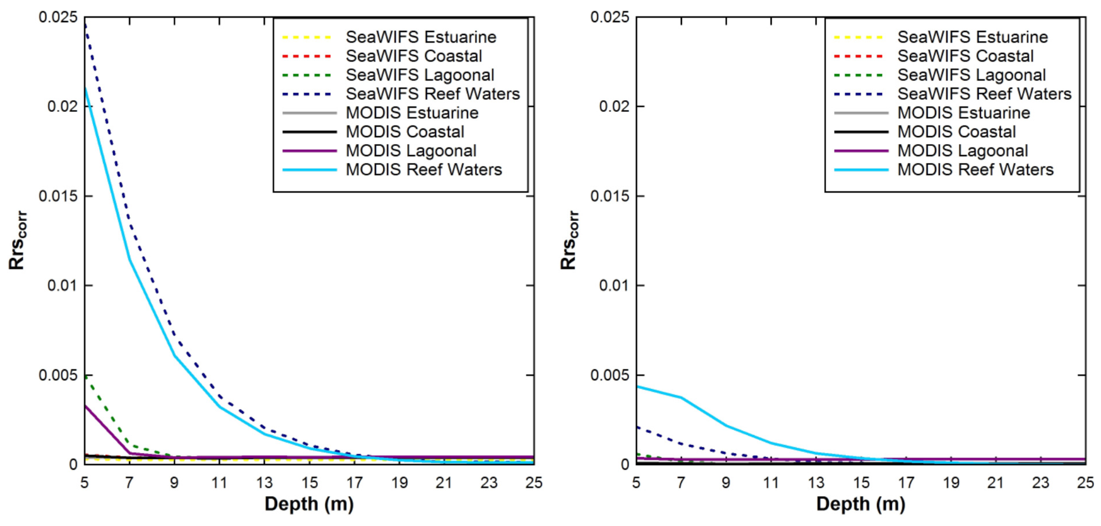
This study assessed the influence of bottom reflectance on the spectrally-averaged R_rs signal measured by the moderate resolution SeaWiFS and MODIS sensors in optically shallow waters of coral reef environments. The results showed: (i) that there was no significant (R_rscorr < 0.0005 sr⁻¹) influence of bottom reflectance on the R_rs signal for depths >19 m for either sensor; and (ii) that the assessed bottom cover classes can be amalgamated into two distinct functional groups, “light” and “dark”, based on the modeled R_rs surface reflectance signals. Only R_rs spectra dominated by light sand and its mixtures can be clearly discriminated from other bottom cover types typically found in coral reef waters.

SeaWiFS and MODIS R_rs data are routinely used to derive IOPs and a number of IOP-based geophysical products such as Chla and the diffuse attenuation coefficient (K_d). Light reflected off the seafloor in optically shallow waters contaminates the sensor-observed R_rs signal and subsequently causes errors in the derived IOPs. The recently-developed semi-analytical SWIM algorithm was specifically devised to improve IOP retrievals in optically shallow coral reef waters, such as the GBR. An essential input component of the SWIM algorithm is a bottom reflectance map [17]. To construct a bottom reflectance map, it is essential to know the number of distinct spectral classes to be mapped and which spectra best represent these classes [17]. Further, it is useful to know in which geographic areas bottom reflectance is most likely to contaminate R_rs and therefore needs to be included in the bottom reflectance map. To address this, we determined the maximum geometric depth at which bottom reflectance may be detectable under different IOP/water clarity scenarios.

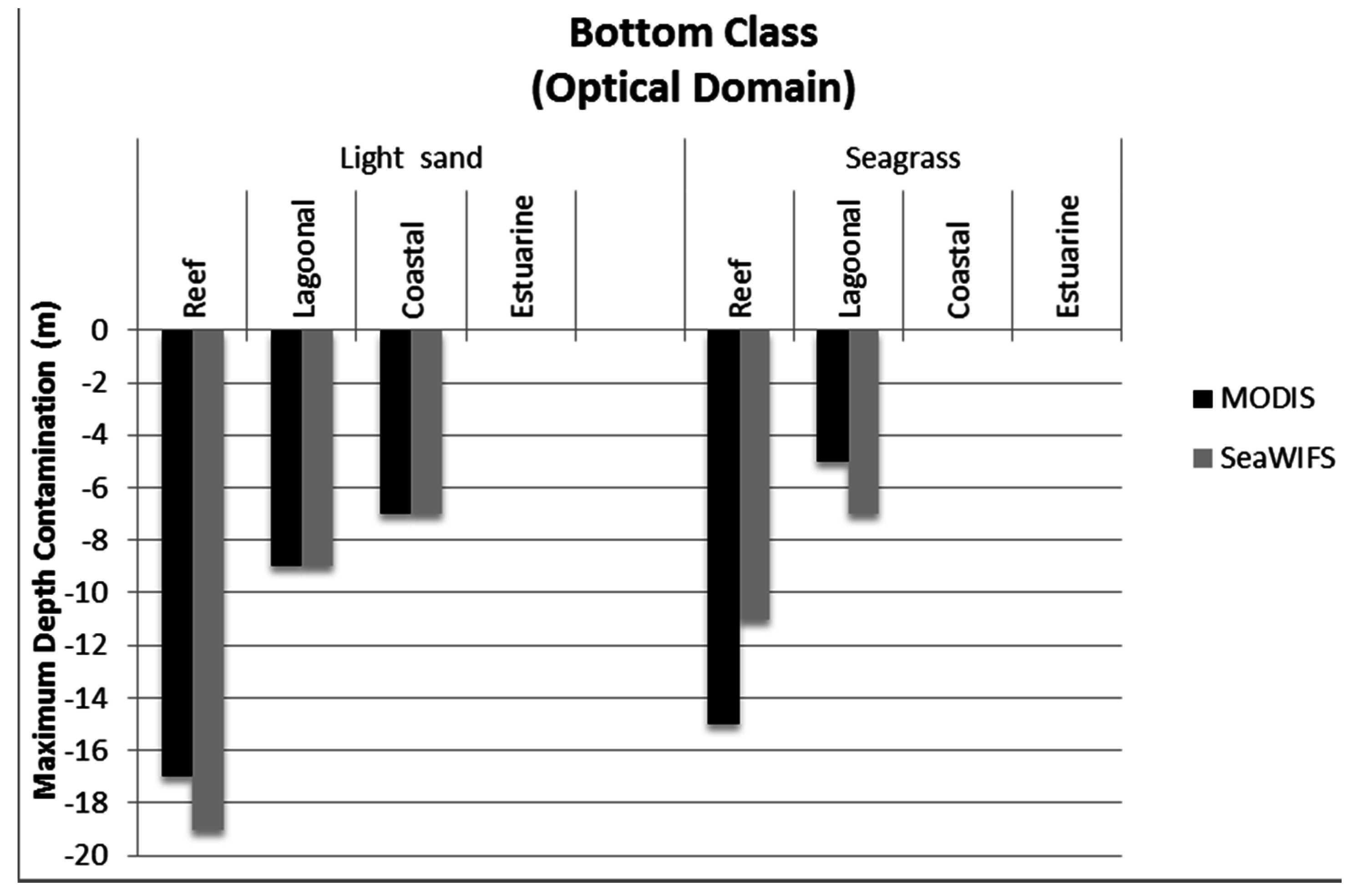
The maximum depth of bottom detectability for clear reefal waters of the GBR was determined to be 17 m and 19 m for spectrally-averaged MODIS band SeaWiFS bands, respectively. However, the depth of bottom detectability was reduced substantially in highly attenuating, inshore waters. Hence the SWIM algorithm may not need to account for bottom reflectance where the water column depth exceeds 19 m. We found bottom reflectance from seagrass, a relatively dark substrate, had no influence on spectrally-averaged R_rs at depths exceeding 15 m for MODIS bands and depths exceeding 11 m for SeaWiFS. 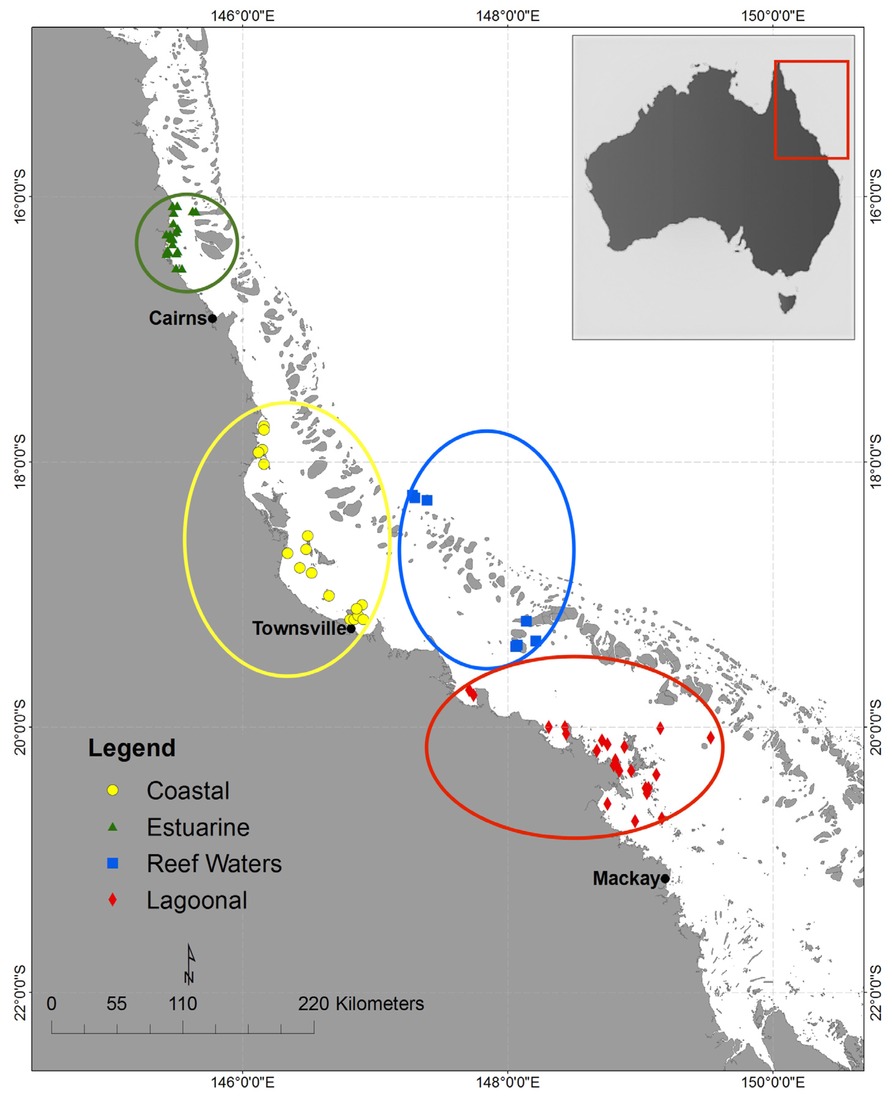Seagrass occurrence is prevalent in coral reef waters and has been recorded down to depths of 61 m in the GBR [54]. In Estuarine waters, which are dominated by terrigenous runoff, particularly in the summer wet season, bottom reflectance contamination was found to be minimal and undetectable in waters >5 m. In Coastal water types, darker bottom covers such as seagrass were also undetectable at depths >5 m.

The minor differences in the maximum depth of bottom detectability between MODIS and SeaWiFS may be explained by the placement of their spectral bands. For example, for Reef Waters using the light sand bottom spectra, SeaWiFS provided a slightly deeper maximum depth than MODIS (19 m vs. 17 m), which is likely due to the placement and width of the assessed bands. The differences in the bands 490/488 (SeaWiFS band 3 and MODIS/Aqua band 10, respectively) and 555/551 (SeaWiFS band 5 and MODIS/Aqua band 12, respectively) result in different radiance retrievals for these blue-green bands [55], which may have caused the minor differences in maximum depth of detectability. Further, the minor difference in maximum depth of bottom reflectance detectability might be due to band-averaging, as MODIS has two red bands compared to one for SeaWiFS. In addition, our study used 2 m depth increments, thus the real difference in maximum depth of bottom reflectance detectability lies within a 0–2 m depth range. Even a 2 m depth difference in a 1km × 1 km pixel is relatively minor and is not expected to make much difference to IOP retrievals using semi-analytical inversion algorithms.

We focused on the band-averaged maximum depth of bottom reflectance detectability to investigate to which depth MODIS and SeaWiFS satellite sensors could detect bottom signals affecting shallow water inversion models. We selected a cutoff threshold of 0.00005 sr⁻¹, which was 2% of the maximum, band-averaged, modeled remote sensing reflectance, 0.025 sr⁻¹. Anything below this threshold was considered noise. Therefore, one could argue that no signal from the bottom was recorded below this threshold. However, a minimal influence of benthic albedo was detected at the red bands (>650 nm), where pure water absorption is high. The bottom reflectance contribution was primarily detected in bands at 488 nm, 531 nm and 551 nm for modeled MODIS R_rs and at 490 nm, 510 nm and 555 nm for modeled SeaWiFS R_rs.

The four optical environments used in this study are defined on the basis of chlorophyll, suspended matter and CDOM, rather than on the optical properties themselves. We acknowledge that the simulations of the optical properties are computed within HE5, using conversions to absorption, scattering and backscattering, and therefore may not be always appropriate in coastal waters.

Further, it should be noted that at the resolution of MODIS and SeaWiFS, one would expect mixed depth pixels, as well as mixed bottom types. This might lead to increasing or decreasing detectability and separability of bottom types and thus lead to uncertainties in IOP retrievals.

However, to date there are no studies known to the authors that have ascertained the maximum depth at which MODIS or SeaWiFS-observed R_rs are contaminated by benthic reflectance despite these moderate resolution sensors being commonly used in near-coastal waters by the international scientific community. Some recently developed ocean color shallow water inversion models that retrieve IOPs, such as SWIM, require input of bottom reflectance parameters as model input. Hence, determining the maximum depth of bottom detection at moderate resolution sensor bands is essential to the implementation of shallow water inversion models to coral reef ecosystems.

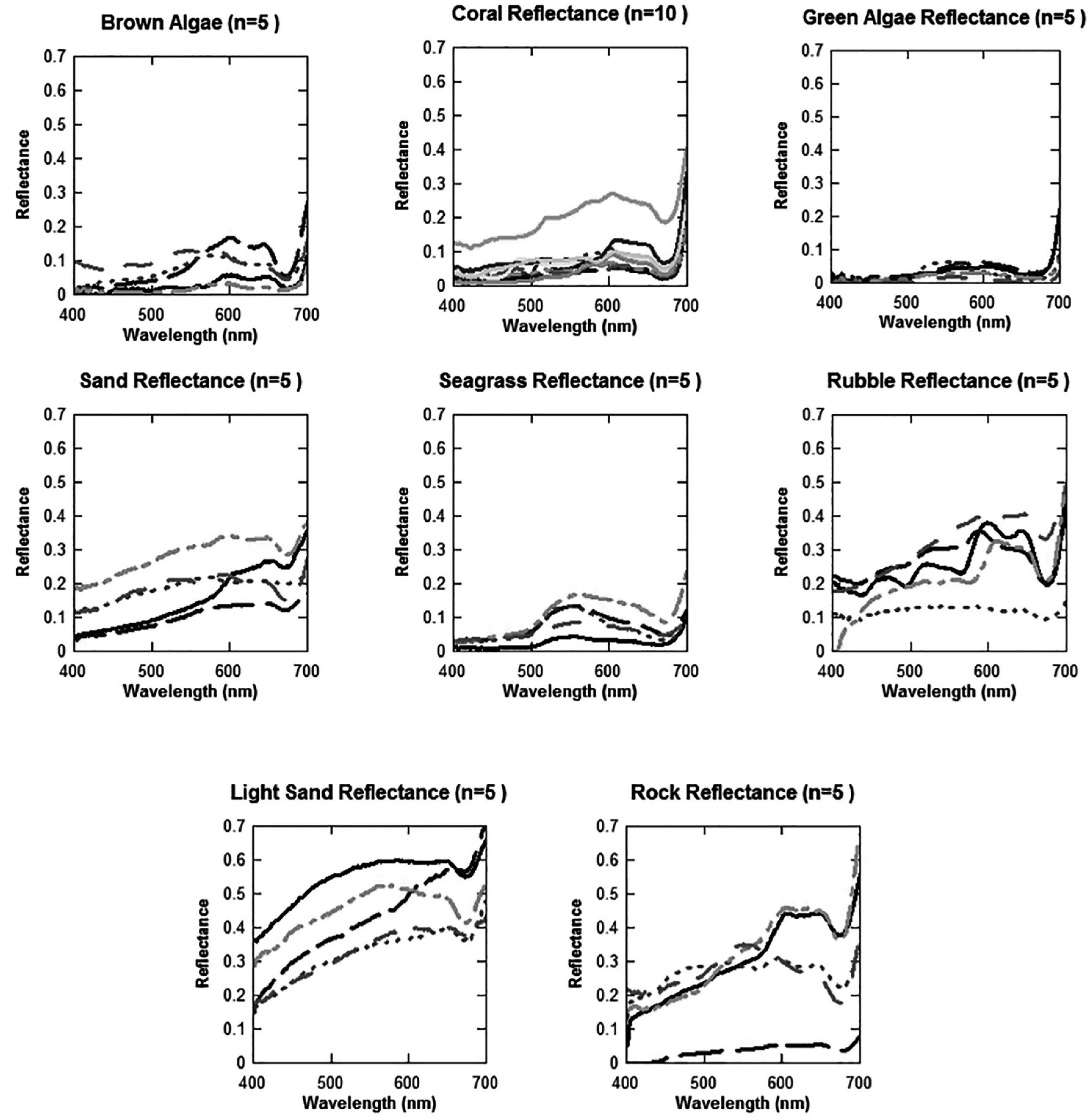
Here, we presented the maximum depth of bottom reflectance contribution to spectrally-averaged R_rs for light sand and seagrass spectra only. We found these to represent two contrasting groups in coral reef waters, light versus dark substrates, based on their average spectral reflectance. Seagrass best represented the dark spectra group for the GBR as seagrass meadows can be thick and extensive there. Besides being the most common bottom cover of the dark spectral group in the GBR, seagrass is also closest to the average spectra of the dark spectral group. In the GBR, seagrass accounts for an estimated 40,000 km² of bottom cover [56] compared to coral reef and algae cover of ~24,158 km² [57], with the remaining ~280,242 km² (81%) of the GBR Marine Park comprising primarily sand and mud.

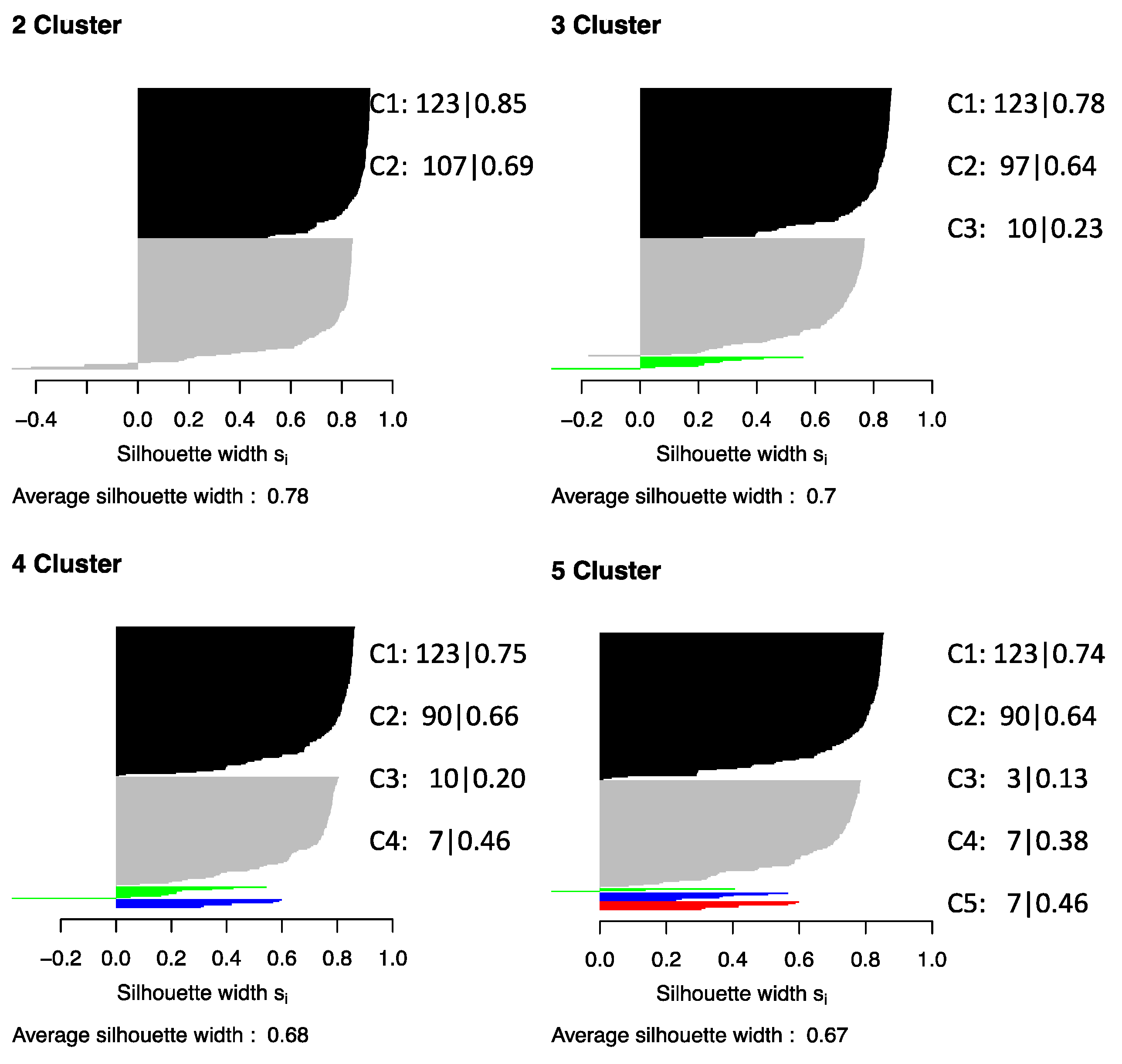
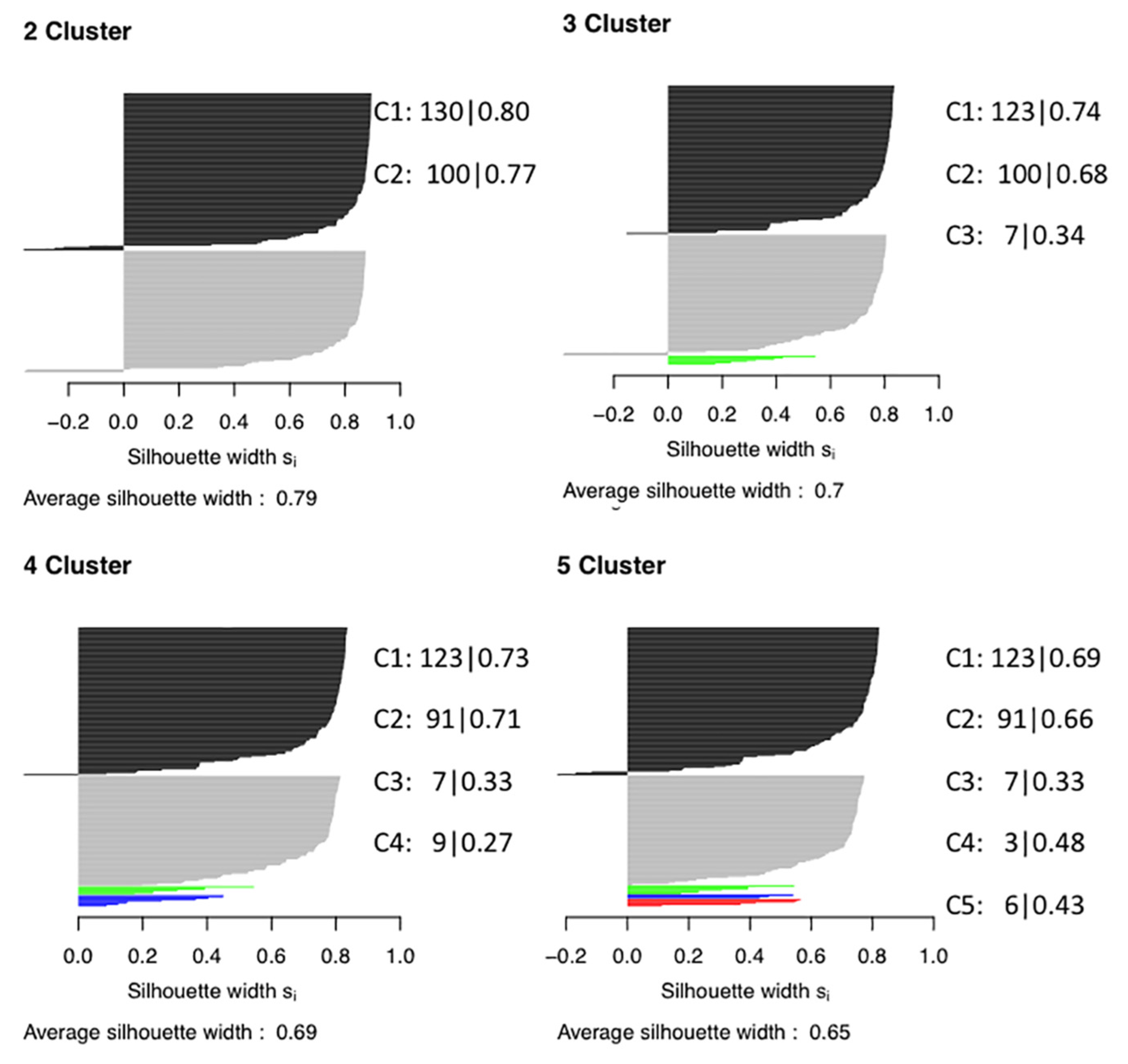
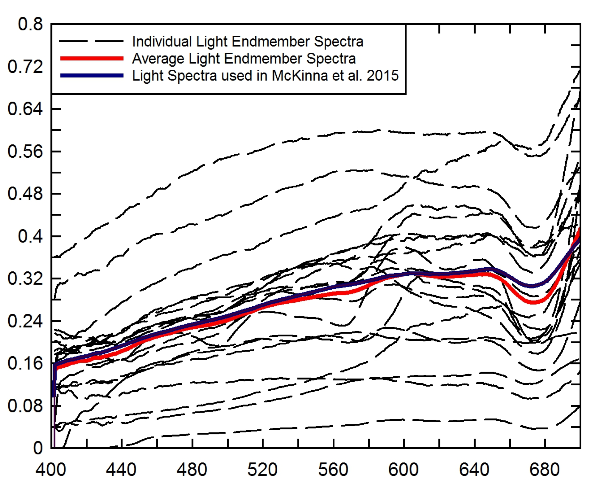
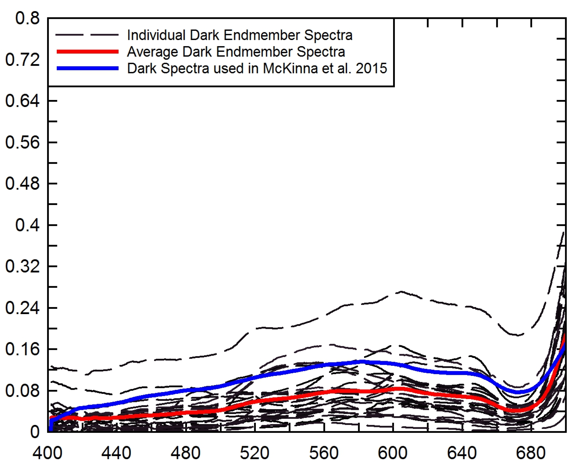
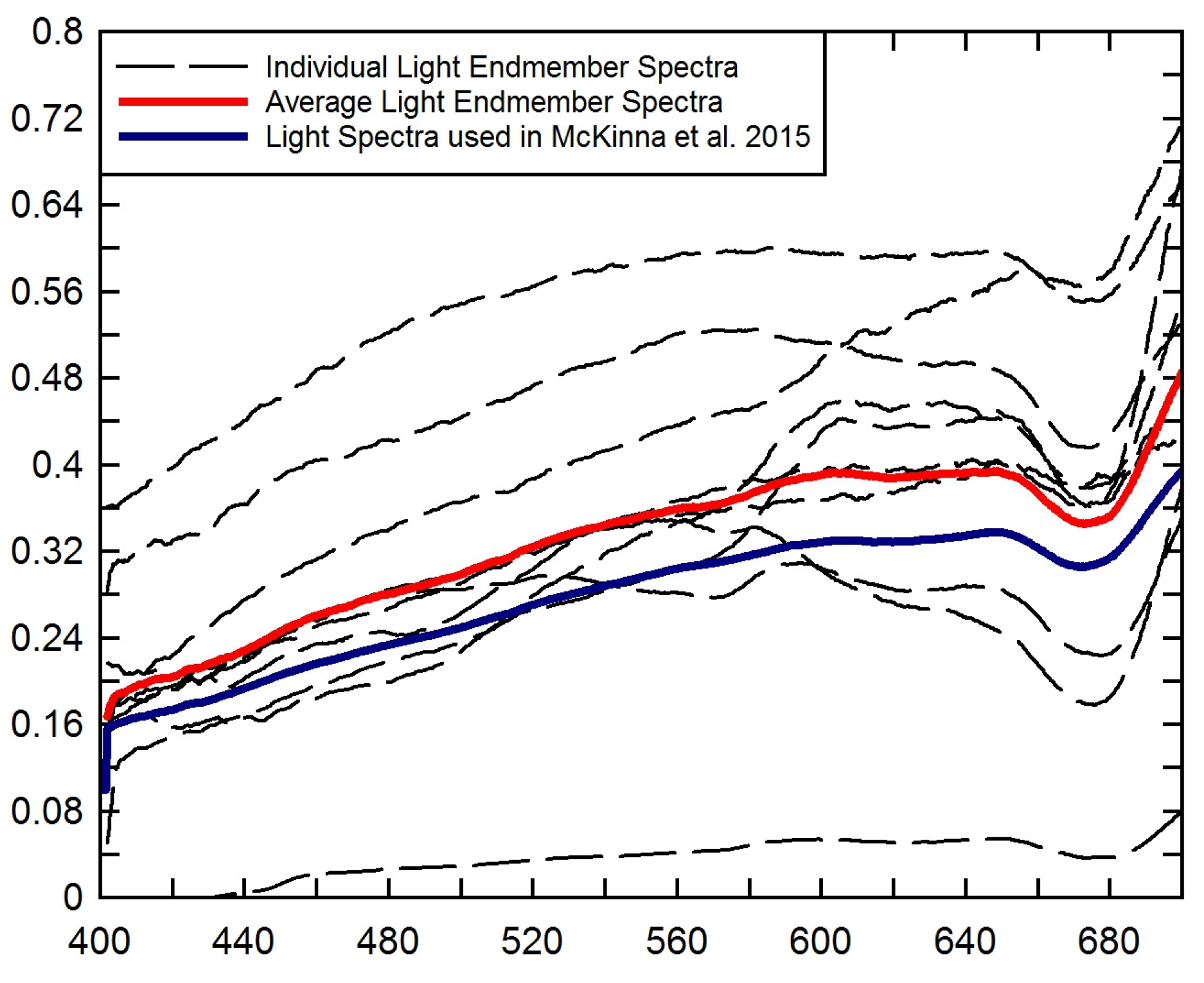
Clustering analysis showed that a two-cluster bottom reflectance input configuration, light and dark, is sufficient for parameterizing a shallow water inversion algorithm for MODIS and SeaWiFS sensors. Assessment of spectral uniqueness based on clustering showed that more clusters resulted in weak cluster structures and misclassified bottom types. Using several spectral samples for each bottom reflectance class allowed us to examine whether particular bottom classes might be ambiguously assigned to a specific cluster and hence misclassified. Modeled R_rs signals at MODIS bands assigned to two primary clusters allowed more consistent grouping of the individual bottom reflectances, with less bottom classes assigned to an “intermediary” cluster group, than at SeaWiFS bands. The intermediary cluster group contained bottom classes that could not be clearly assigned to C1 (dark) or C2 (light) because some of the five (ten for coral) spectral samples from one bottom class were assigned to C1 while others were assigned to C2. Using SeaWiFS bands, the majority of sand and rubble classes could not be clearly assigned to C1 or C2 as their spectral signatures lay between C1 and C2 (not as light as light sand but also not as dark as seagrass or similar). For either sensor, there was no bottom reflectance detected from seagrass for the Coastal or Estuarine optical scenarios, where the water is turbid, even at a shallow depth of 5 m. However, bottom contamination from light sand was still recorded in coastal waters by MODIS. The results provide insight into the optimal substrate clustering for bottom reflectance parameterization in shallow water models. The endmember and average spectra for the light and dark clusters are presented in the Appendix.

To date, there have been no bottom cover spectral reflectance studies focusing on spectral separability or spectral uniqueness of bottom reflectance spectra at MODIS or SeaWiFS spectral and spatial resolutions known to the authors. Indeed, most comparative studies of bottom reflectance in shallow waters have focused on habitat classification mapping, e.g., [26,38,58,59,60]) that requires a greater level of spatial and spectral detail. Generally, research on substrate spectral uniqueness has been undertaken using sensors with higher spatial resolution (pixel size < 50 m and mostly < 4 m) as they are commonly used to map benthic habitat or bathymetry at higher resolution, e.g., [15,28,29,61,62]). The spatial area imaged by these sensors is typically much smaller than the scale of larger coral reef ecosystems such as the GBR. Most high spatial resolution multi- and hyperspectral satellite-borne sensors do not have the temporal or spatial coverage provided by MODIS and SeaWiFS. Indeed, the broad swath and regular repeat orbits afforded by MODIS and SeaWiFS are needed to monitor and manage the ecosystem health of the GBR waters on a near-daily basis.

Higher resolution sensors are typically able to discern smaller objects and image pixels often contain signals from a single substrate class. These smaller objects cannot be distinguished by MODIS or SeaWiFS satellite sensors, as image pixels frequently contain signals from a mixture of substrate types. In order for a homogeneous bottom cover to contribute to sensor-observed R_rs, its size has to be larger than several pixels in a specific satellite image. We made the assumption that, if the bottom cover extent was smaller than the pixel size, the signal detected represented the average brightness of all bottom covers in that pixel. Nevertheless, smaller percentages of particular types of bottom cover, such as small patches of sand between extensive seagrass beds, may be detectable if their reflectance signal dominates a particular pixel. MODIS and SeaWiFS have a coarser spatial resolution than most of the commonly used higher resolution satellite sensors (such as IKONOS, WorldView2, etc.). Thus, bottom covers considered in this study generally occur on spatial scales > 1000 m and are not based on specific species per habitat classification, but rather classified into broader bottom classes, such as algae. A number of pure endmember bottom spectra were combined into mixed bottom types most commonly observed in the GBR at MODIS and SeaWiFS scales.

From an ocean color perspective, we may consider the GBR to be divided into three distinct zones based on water depth and geological features: (1) an inner shelf zone with a depth range of 0–20 m dominated by terrigenous sediment; (2) a middle shelf zone with a depth range of 20–40 m of mixed carbonate-siliciclastic sediment; and (3) an outer shelf zone with a depth range of 40–90 m of carbonate-dominated sediment [63,64]. The maximum depth of bottom contamination of 19 m found in this study corresponds primarily to the inner shelf region of 0–20 m. This region, with a width of <60 km, is therefore of primary concern for benthic contamination in ocean color algorithms. Because of resuspension and other processes, this is also the zone where optically complex ocean color remote sensing challenges are the greatest. However, our results showed that the most significant bottom contamination is recorded from light (carbonate) sand, which is mainly found in the middle and outer shelf zones of the GBR [65]. Hence, this study suggests that the primary areas of concern for benthic contamination of the R_rs signal may be shallow waters adjacent to coral reefs on the mid- to outer shelf of the GBR, rather than the shallow inner shelf region.

5. Conclusions

This study has considered spectral separability or classification in the context of improving bottom cover benthic albedo (reflectance) parameterization in shallow water inversion models. To date ocean color algorithms have primarily been developed for moderate resolution sensors, such as MODIS or SeaWiFS, which are typically employed to provide data on the global oceans on a daily basis. It is well known by the research community that the frequency and placement of the current ocean color satellite sensor bands are inadequate and do not capture most of the variability of the remote sensing reflectance caused by differences in IOPs and bottom cover [22,66,67,68]. This study confirms that the separability of common bottom covers is limited using the existing set of visible bands of the MODIS and SeaWiFS satellite sensors. The only bottom cover group that could be confidently separated from other bottom cover classes was light sand and its mixtures. This separability deteriorated in Lagoonal and Coastal water optical scenarios. In Estuarine waters, no bottom cover class could be separated even though some bottom contamination was recorded up to 5 m depth. These findings are consistent with previous studies that noted that light and dark features can be separated, but finer class separability would require higher spectral resolution [29]. The results show that bottom reflectance in shallow water models only needs to be considered up to 19 m depth for MODIS and SeaWiFS based on spectrally averaged results. This would exclude a large area of the GBR, and similarly of other coral reef systems, which are deeper than 19 m and hence, not significantly affected by bottom reflectance. In addition, we can conclude that only two spectral signatures have to be considered in the parameterization of bottom reflectance in shallow water inversion algorithms when applied to sensors such as SeaWiFS and MODIS. A light and a dark spectral signature should provide sufficient detail to improve the IOP retrievals. The outcomes of this work will guide the development of improved bottom reflectance datasets required by shallow water ocean color inversion algorithms such as SWIM. Such improved parameterization will assist in better estimating how much light is reflected from the bottom, contaminating ocean color satellite imagery used for water clarity monitoring, and thus lead to improved retrievals of IOPs and water column constituent concentrations.

References

1. Fabricius, K.E. Effects of terrestrial runoff on the ecology of corals and coral reefs: Review and synthesis. Mar. Pollut. Bull. 2005, 50, 125–146. [Google Scholar] [CrossRef] [PubMed]
2. Weeks, S.; Werdell, P.J.; Schaffelke, B.; Canto, M.; Lee, Z.; Wilding, J.G.; Feldman, G.C. Satellite-derived photic depth on the great barrier reef: Spatio-temporal patterns of water clarity. Remote Sens. 2012, 4, 3781–3795. [Google Scholar] [CrossRef]
3. Loisel, H.; Vantrepotte, V.; Jamet, C.; Dat, D.N. Challenges and new advances in ocean color remote sensing of coastal waters. In Topics in Oceanography; Intech: Rijeka, Croatia, 2013; pp. 953–980. [Google Scholar]
4. Mobley, C.; Boss, E.; Roesler, C. Ocean Optics Web Book. 2010. Available online: http://www.oceanopticsbook.info (accessed on 10 June 2015).
5. O‘Reilly, J.E.; Maritorena, S.; Mitchell, B.G.; Siegel, D.A.; Carder, K.L.; Garver, S.A.; Kahru, M.; McClain, C. Ocean color chlorophyll algorithms for SeaWiFS. J. Geophys. Res. Oceans 1998, 103, 24937–24953. [Google Scholar] [CrossRef]
6. Lee, Z.; Carder, K.L.; Arnone, R.A. Deriving inherent optical properties from water color: A multiband quasi-analytical algorithm for optically deep waters. Appl. Opt. 2002, 41, 5755–5772. [Google Scholar] [CrossRef] [PubMed]
7. Werdell, P.J.; Bailey, S.W. An improved in-situ bio-optical data set for ocean color algorithm development and satellite data product validation. Remote Sens. Environ. 2005, 98, 122–140. [Google Scholar] [CrossRef]
8. Maritorena, S.; Siegel, D.A.; Peterson, A.R. Optimization of a semianalytical ocean color model for global-scale applications. Appl. Opt. 2002, 41, 2705–2714. [Google Scholar] [CrossRef] [PubMed]
9. Bierwirth, P.; Lee, T.; Burne, R. Shallow sea-floor reflectance and water depth derived by unmixing multispectral imagery. Photogramm. Eng. Remote Sens. 1993, 59, 331–338. [Google Scholar]
10. Dierssen, H.M.; Zimmerman, R.C.; Leathers, R.A.; Downes, T.V.; Davis, C.O. Ocean color remote sensing of seagrass and bathymetry in the Bahamas Banks by high-resolution airborne imagery. Limnol. Oceanogr. 2003, 48, 444–455. [Google Scholar] [CrossRef]
11. Louchard, E.M.; Reid, R.P.; Stephens, F.C.; Davis, C.O.; Leathers, R.A.; Downes, T.V. Optical remote sensing of benthic habitats and bathymetry in coastal environments at Lee Stocking Island, Bahamas: A comparative spectral classification approach. Limnol. Oceanogr. 2003, 48, 511–521. [Google Scholar]
12. Werdell, P.J.; Roesler, C.S. Remote assessment of benthic substrate composition in shallow waters using multispectral reflectance. Limnol. Oceanogr. 2003, 48, 557–567. [Google Scholar] [CrossRef]
13. Lee, Z.; Hu, C.; Casey, B.; Shang, S.; Dierssen, H.; Arnone, R. Global shallow water bathymetry from satellite ocean color data. Eos Trans. Am. Geophys. Union 2010, 91, 429–430. [Google Scholar] [CrossRef]
14. Wettle, M.; Brando, V.E. SAMBUCA: Semi-Analytical Model for Bathymetry, Un-Mixing and Concentration Assessment; CSIRO Land and Water: Canberra, ACT, Austrilia, 2006. [Google Scholar]
15. Dekker, A.G.; Phinn, S.R.; Anstee, J.; Bissett, P.; Brando, V.E.; Casey, B.; Fearns, P.; Hedley, J.; Klonowski, W.; Lee, Z.P. Intercomparison of shallow water bathymetry, hydro-optics, and benthos mapping techniques in Australian and Caribbean coastal environments. Limnol. Oceanogr. Methods 2011, 9, 396–425. [Google Scholar] [CrossRef]
16. Barnes, B.B.; Hu, C.; Schaeffer, B.A.; Lee, Z.; Palandro, D.A.; Lehrter, J.C. MODIS-derived spatiotemporal water clarity patterns in optically shallow Florida Keys waters: A new approach to remove bottom contamination. Remote Sens. Environ. 2013, 134, 377–391. [Google Scholar] [CrossRef]
17. McKinna, L.I.W.; Fearns, P.R.C.; Weeks, S.J.; Werdell, P.J.; Reichstetter, M.; Franz, B.A.; Shea, D.M.; Feldman, G.C. A semianalytical ocean color inversion algorithm with explicit water column depth and substrate reflectance parameterization. J. Geophys. Res. Oceans 2015, 120, 1741–1770. [Google Scholar] [CrossRef]
18. Lee, Z.; Carder, K.L.; Mobley, C.D.; Steward, R.G.; Patch, J.S. Hyperspectral remote sensing for shallow waters. I. A semianalytical model. Appl. Opt. 1998, 37, 6329–6338. [Google Scholar] [CrossRef] [PubMed]
19. Beaman, R. Great Barrier Reef and Coral Sea Bathymetry. Available online: http://deepreef.org/bathymetry.html (accessed on 14 December 2012).
20. Pitcher, C.R.; Doherty, P.; Arnold, P.; Hooper, J.; Gribble, N.; Bartlett, C.; Browne, M.; Campbell, N.; Cannard, T.; Cappo, M.; et al. Seabed Biodiversity on the Continental Shelf of the Great Barrier Reef World Heritage Area; CSIRO Marine and Atmospheric Research: Canberra, ACT, Austrilia, 2007. [Google Scholar]
21. Reichstetter, M.; McKinna, L.; Fearns, P.; Weeks, S.J.; Roelfsema, C.M.; Furnas, M. Seafloor Brightness Map of the Great Barrier Reef, Australia, Derived from Biodiversity Data; Pangaea: Bremerhaven, Germany, 2015. [Google Scholar]
22. Lee, Z.; Carder, K.; Arnone, R.; He, M. Determination of primary spectral bands for remote sensing of aquatic environments. Sensors 2007, 7, 3428–3441. [Google Scholar] [CrossRef]
23. Malenovský, Z.; Rott, H.; Cihlar, J.; Schaepman, M.E.; García-Santos, G.; Fernandes, R.; Berger, M. Sentinels for science: Potential of Sentinel-1, -2, and-3 missions for scientific observations of ocean, cryosphere, and land. Remote Sens. Environ. 2012, 120, 91–101. [Google Scholar] [CrossRef]
24. Andréfouët, S.; Muller-Karger, F.E.; Hochberg, E.J.; Hu, C.; Carder, K.L. Change detection in shallow coral reef environments using Landsat 7 ETM+ data. Remote Sens. Environ. 2001, 78, 150–162. [Google Scholar] [CrossRef]
25. Hochberg, E.J.; Atkinson, M.J.; Apprill, A.; Andrefouet, S. Spectral reflectance of coral. Coral Reefs 2004, 23, 84–95. [Google Scholar] [CrossRef]
26. Holden, H.; LeDrew, E. Spectral discrimination of healthy and non-healthy corals based on cluster analysis, principal components analysis, and derivative spectroscopy. Remote Sens. Environ. 1998, 65, 217–224. [Google Scholar] [CrossRef]
27. Joyce, K.; Phinn, S.; Roelfsema, C.; Neil, D.; Dennison, W. Combining Landsat ETM+ and reef check classifications for mapping coral reefs: A critical assessment from the southern Great Barrier Reef, Australia. Coral Reefs 2004, 23, 21–25. [Google Scholar] [CrossRef]
28. Kutser, T.; Miller, I.; Jupp, D.L.B. Mapping coral reef benthic substrates using hyperspectral space-borne images and spectral libraries. Estuar. Coast. Shelf Sci. 2006, 70, 449–460. [Google Scholar] [CrossRef]
29. Botha, E.J.; Brando, V.E.; Anstee, J.M.; Dekker, A.G.; Sagar, S. Increased spectral resolution enhances coral detection under varying water conditions. Remote Sens. Environ. 2013, 131, 247–261. [Google Scholar] [CrossRef]
30. Hedley, J.D.; Roelfsema, C.M.; Phinn, S.R.; Mumby, P.J. Environmental and sensor limitations in optical remote sensing of coral reefs: Implications for monitoring and sensor design. Remote Sens. 2012, 4, 271–302. [Google Scholar] [CrossRef]
31. Leiper, I.; Phinn, S.; Dekker, A.G. Spectral reflectance of coral reef benthos and substrate assemblages on Heron Reef, Australia. Int. J. Remote Sens. 2011, 33, 3946–3965. [Google Scholar] [CrossRef]
32. Mobley, C.D.; Sundman, L.K. Hydrolight 5 Ecolight 5 Users’ Guide; Sequoia Scientific Inc: Bellvue, WA, USA, 2008. [Google Scholar]
33. Roelfsema, C.M.; Phinn, S.R. Spectral Reflectance Library of Selected Biotic and Abiotic Coral Reef Features in Heron Reef; Pangaea: Bremerhaven, Germany, 2012. [Google Scholar]
34. Roelfsema, C.M.; Phinn, S.R. Spectral Reflectance Library of Selected Biotic and Abiotic Coral Reef Features in Glovers Reef, Belize; Pangaea: Bremerhaven, Germany, 2013. [Google Scholar]
35. Roelfsema, C. Spectral Reflectance Library; University of Queensland: Queensland, QLD, Australia, 2012. [Google Scholar]
36. Blondeau-Patissier, D.; Brando, V.E.; Oubelkheir, K.; Dekker, A.G.; Clementson, L.A.; Daniel, P. Bio-optical variability of the absorption and scattering properties of the Queensland inshore and reef waters, Australia. J. Geophys. Res. Oceans 2009, 114. [Google Scholar] [CrossRef]
37. Kutser, T.; Jupp, D.L. On the possibility of mapping living corals to the species level based on their optical signatures. Estuar. Coast. Shelf Sci. 2006, 69, 607–614. [Google Scholar] [CrossRef]
38. Hochberg, E.J.; Atkinson, M.J.; Andréfouėt, S. Spectral reflectance of coral reef bottom-types worldwide and implications for coral reef remote sensing. Remote Sens. Environ. 2003, 85, 159–173. [Google Scholar] [CrossRef]
39. Hedley, J.D.; Mumby, P.J.; Joyce, K.E.; Phinn, S.R. Spectral unmixing of coral reef benthos under ideal conditions. Coral Reefs 2004, 23, 60–73. [Google Scholar] [CrossRef]
40. Hedley, J.D.; Mumby, P.J. Biological and remote sensing perspectives of pigmentation in coral reef organisms. Adv. Mar. Biol. 2002, 43, 277–317. [Google Scholar] [PubMed]
41. Gardner, W. Measurement of spectral correlation. IEEE Trans. Acoust. Speech Signal Process. 1986, 34, 1111–1123. [Google Scholar] [CrossRef]
42. Casal, G.; Kutser, T.; Domínguez-Gómez, J.; Sánchez-Carnero, N.; Freire, J. Mapping benthic macroalgal communities in the coastal zone using CHRIS-PROBA mode 2 images. Estuar. Coast. Shelf Sci. 2011, 94, 281–290. [Google Scholar] [CrossRef]
43. Karpouzli, E.; Malthus, T.; Place, C. Hyperspectral discrimination of coral reef benthic communities in the western Caribbean. Coral Reefs 2004, 23, 141–151. [Google Scholar] [CrossRef]
44. Van Der Meer, F. Iterative spectral unmixing (ISU). Int. J. Remote Sens. 1999, 20, 3431–3436. [Google Scholar] [CrossRef]
45. Goodman, J.; Ustin, S.L. Classification of benthic composition in a coral reef environment using spectral unmixing. J. Appl. Remote Sens. 2007, 1. [Google Scholar] [CrossRef]
46. Sohn, Y.; Rebello, N.S. Supervised and unsupervised spectral angle classifiers. Photogramm. Eng. Remote Sens. 2002, 68, 1271–1282. [Google Scholar]
47. Keshava, N. Distance metrics and band selection in hyperspectral processing with applications to material identification and spectral libraries. IEEE Trans. Geosci. Remote Sens. 2004, 42, 1552–1565. [Google Scholar] [CrossRef]
48. Kruse, F.A.; Boardman, J.W.; Huntington, J.F. Comparison of airborne hyperspectral data and EO-1 Hyperion for mineral mapping. IEEE Trans. Geosci. Remote Sens. 2003, 41, 1388–1400. [Google Scholar] [CrossRef]
49. Sohn, Y.; Moran, E.; Gurri, F. Deforestation in North-Central Yucatan(1985–1995): Mapping secondary succession of forest and agricultural land use in Sotuta using the cosine of the angle concept. Photogramm. Eng. Remote Sens. 1999, 65, 947–958. [Google Scholar]
50. Lass, L.W.; Thill, D.C.; Shafii, B.; Prather, T.S. Detecting Spotted Knapweed (Centaurea maculosa) with Hyperspectral Remote Sensing Technology. Weed Technol. 2002, 16, 426–432. [Google Scholar] [CrossRef]
51. Kaufman, L.; Rousseeuw, P.J. Finding Groups in Data: An Introduction to Cluster Analysis; John Wiley & Sons: Hoboken, NY, USA, 2009. [Google Scholar]
52. Batagelj, V. Generalized ward and related clustering problems. In Classification and Related Methods of Data Analysis; North-Holland: Amsterdam, the Netherlands, 1988; pp. 67–74. [Google Scholar]
53. Rousseeuw, P.J. Silhouettes: A graphical aid to the interpretation and validation of cluster analysis. J. Comput. Appl. Math. 1987, 20, 53–65. [Google Scholar] [CrossRef]
54. Coles, R.; McKenzie, L.; De’ath, G.; Roelofs, A.; Lee Long, W. Spatial distribution of deepwater seagrass in the inter-reef lagoon of the Great Barrier Reef World Heritage Area. Mar. Ecol. Prog. Ser. 2009, 392, 57–68. [Google Scholar] [CrossRef]
55. Franz, B.A.; Werdell, P.J.; Meister, G.; Bailey, S.W.; Eplee, R.E., Jr.; Feldman, G.C.; Kwiatkowskaa, E.; McClain, C.R.; Patt, F.S.; Thomas, D. The continuity of ocean color measurements from SeaWiFS to MODIS. In Proceedings of the 2005 International Society for Optics and Photonic, San Diego, CA, USA, 31 July–4 August 2005.
56. Schaffelke, B.; Mellors, J.; Duke, N.C. Water quality in the Great Barrier Reef region: Responses of mangrove, seagrass and macroalgal communities. Mar. Pollut. Bull. 2005, 51, 279–296. [Google Scholar] [CrossRef] [PubMed]
57. Beaman, R.J. Project 3DGBR: A High-Resolution Depth Model for the Great Barrier Reef and Coral Sea; Marine and Tropical Sciences Facility (MTSRF): Cairns, QLA, Austrilia, 2010. [Google Scholar]
58. Mumby, P.; Green, E.; Edwards, A.; Clark, C. Coral reef habitat mapping: How much detail can remote sensing provide? Mar. Biol. 1997, 130, 193–202. [Google Scholar] [CrossRef]
59. Hochberg, E.J.; Atkinson, M.J. Capabilities of remote sensors to classify coral, algae, and sand as pure and mixed spectra. Remote Sens. Environ. 2003, 85, 174–189. [Google Scholar] [CrossRef]
60. Kutser, T.; Dekker, A.G.; Skirving, W. Modeling spectral discrimination of Great Barrier Reef benthic communities by remote sensing instruments. Limnol. Oceanogr. 2003, 48, 497–510. [Google Scholar] [CrossRef]
61. Mishra, D.; Narumalani, S.; Rundquist, D.; Lawson, M. Benthic habitat mapping in tropical marine environments using QuickBird multispectral data. Photogramm. Eng. Remote Sens. 2006, 72, 1037–1048. [Google Scholar] [CrossRef]
62. Stumpf, R.P.; Holderied, K.; Sinclair, M. Determination of water depth with high-resolution satellite imagery over variable bottom types. Limnol. Oceanogr. 2003, 48, 547–556. [Google Scholar] [CrossRef]
63. Belperio, A.; Searle, D. Terrigenous and carbonate sedimentation in the Great Barrier Reef province. Dev. Sedimentol. 1988, 42, 143–174. [Google Scholar]
64. Mathews, E.; Heap, A.; Woods, M. Inter-Reefal Seabed Sediments and Geomorphology of the Great Barrier Reef: A Spatial Analysis; Geoscience Australia: Canberra, ACT, 2007; p. 140. [Google Scholar]
65. Belperio, A. Terrigenous sedimentation in the central Great Barrier Reef lagoon: A model from the Burdekin region. BMR J. Aust. Geolog Geophys. 1983, 8, 179–190. [Google Scholar]
66. Lee, Z.; Carder, K.L. Effect of spectral band numbers on the retrieval of water column and bottom properties from ocean color data. Appl. Opt. 2002, 41, 2191–2201. [Google Scholar] [CrossRef] [PubMed]
67. Decker, A.; Malthus, T.; Wijnen, M.; Seyhan, E. The effect of spectral bandwidth and positioning on the spectral signature analysis of inland waters. Remote Sens. Environ. 1992, 41, 211–225. [Google Scholar] [CrossRef]
68. Wernand, M.; Shimwell, S.; de Munck, J. A simple method of full spectrum reconstruction by a five-band approach for ocean colour applications. Int. J. Remote Sens. 1997, 18, 1977–1986. [Google Scholar] [CrossRef]