Comparison of Spatiotemporal Fusion Models: A Review

Chen, Bin; Huang, Bo; Xu, Bing

doi:10.3390/rs70201798

Open AccessReview

Comparison of Spatiotemporal Fusion Models: A Review

by

Bin Chen

¹

,

Bo Huang

² and

Bing Xu

^1,3,*

¹

State Key Laboratory of Remote Sensing Science, College of Global Change and Earth System Science, Beijing Normal University, Beijing 100875, China

²

Department of Geography and Resource Management and Institute of Space and Earth Information Science, The Chinese University of Hong Kong, Shatin, N.T., Hong Kong

³

Ministry of Education Key Laboratory for Earth System Modelling, Center of Earth System Science, Tsinghua University, Beijing 100084, China

^*

Author to whom correspondence should be addressed.

Remote Sens. 2015, 7(2), 1798-1835; https://0-doi-org.brum.beds.ac.uk/10.3390/rs70201798

Submission received: 8 October 2014 / Accepted: 29 January 2015 / Published: 5 February 2015

Download

Browse Figures

Versions Notes

Abstract

:

Simultaneously capturing spatial and temporal dynamics is always a challenge for the remote sensing community. Spatiotemporal fusion has gained wide interest in various applications for its superiority in integrating both fine spatial resolution and frequent temporal coverage. Though many advances have been made in spatiotemporal fusion model development and applications in the past decade, a unified comparison among existing fusion models is still limited. In this research, we classify the models into three categories: transformation-based, reconstruction-based, and learning-based models. The objective of this study is to (i) compare four fusion models (STARFM, ESTARFM, ISTAFM, and SPSTFM) under a one Landsat-MODIS (L-M) pair prediction mode and two L-M pair prediction mode using time-series datasets from the Coleambally irrigation area and Poyang Lake wetland; (ii) quantitatively assess prediction accuracy considering spatiotemporal comparability, landscape heterogeneity, and model parameter selection; and (iii) discuss the advantages and disadvantages of the three categories of spatiotemporal fusion models.

Keywords:

spatiotemporal fusion; comparison; prediction modes; assessment

1. Introduction

The quantity of remotely sensed data acquired from satellite instruments has greatly increased, contributing to multi-source and multi-resolution image sequences at regional or global scales. However, given the tradeoff between spatial resolution and temporal revisiting cycles [1,2], there is so far no single satellite sensor that can produce images with both fine spatial and temporal resolutions. A comparison of existing sensors and their spatial and temporal resolutions is given in Table 1. For example, SPOT series and Landsat TM/ETM+ multispectral data with spatial resolutions from 6 to 30 m have proven useful in monitoring forest and ecosystem dynamics [3,4,5,6,7], land cover classifications [8,9], and land cover/use change detection [10,11]. However, long revisit frequencies (16 days for Landsat series and 26 days for SPOT), frequent cloud contamination [12], complex topographic effects, and equipment failure make it difficult to acquire sequenced remotely sensed data that target the same region, and have prevented us from applying it to rapid monitoring of disturbance and change detection [2]. In contrast, the NOAA Advanced Very High Resolution Radiometer (AVHRR), SPOT-Vegetation (SOPT-VGT), and Moderate Resolution Imaging Spectroradiometer (MODIS) provide global multispectral imagery of land surface at 1–2-day revisit frequencies [13]. However, their relatively low spatial resolutions, from 250 m to 1 km, are not sufficient for quantitative monitoring of landscape changes that occur at sub-pixel resolutions. A possible cost-effective approach is to generate synthetic data with both fine spatial resolution and temporal frequency by blending the multi-sensor spatial and temporal characteristics. It has aroused great interest within the remote sensing community [2,14,15,16].

Image fusion can be generally divided into spatial and spectral fusion, and spatial and temporal fusion [17]. Spatiospectral fusion, or pan-sharpening, blends a lower spatial resolution multispectral image with a higher spatial resolution panchromatic image. Many spatiospectral fusion models have been developed and have matured during the past three decades. However, spatiospectral fusion methods are not efficient in enhancing the spatial resolution and temporal frequency simultaneously. Spatiotemporal fusion is a relatively new concept addressing this problem. Several spatiotemporal fusion models have been recently proposed. Based on the characteristics of the model framework and procedures for implementing the models, we classify them into three categories: (i) transformation-based; (ii) reconstruction-based; and (iii) learning-based models.

Transformation-based methods include wavelet and tasseled cap transformations [18,19]. Acerbi-Junior et al. [20] increased the spatial resolution of MODIS by integrating Landsat imagery using a three-level coupled wavelet decomposition scheme. Tasseled cap transformation [19] is widely used in detecting land cover change and phenology disturbances [6]. It has been regarded as a standard technique for spectral variation based on the three axes of brightness, greenness, and wetness. Hilker et al. [21] used a tasseled cap transformation of both Landsat TM/ETM+ and MODIS reflectance data to capture change information with a fine spatial resolution in a transformed space.

In reconstruction-based methods, synthetic fusion data are generated by a weighted sum of the spectrally similar neighboring information from fine spatial but coarse temporal resolution, and fine temporal but coarse spatial resolution data [2,15,21]. Gao et al. [2] proposed a spatial and temporal adaptive reflection fusion model (STARFM) to blend Landsat and MODIS imagery to generate daily synthetic Landsat-like data with 30 m spatial resolution. Several improved models have since been developed. Hilker et al. [21] presented a spatial and temporal adaptive algorithm for mapping reflectance change (STAARCH) to identify highly detailed spatiotemporal patterns in land cover change. STAARCH also produces synthetic Landsat-like images for each available date of MODIS data based on an extended STARFM [21]. However, the prediction accuracy of the STARFM and STARRCH models is sensitively correlated with landscape heterogeneity [15]. Based on STARFM, Zhu et al. [15] developed an enhanced spatial and temporal adaptive reflectance fusion model (ESTARFM), considering conversion coefficients, so that homogeneous and heterogeneous pixels have different conversion coefficients in the prediction [22]. Shen et al. [23] proposed an extended spatiotemporal method for reflectance blending prediction within the STARFM framework. It took sensor observation differences for varied land cover types into consideration. However, it requires a prior unsupervised classification for the fine spatial resolution data. A customized blending model was developed by Michishita et al. based on the ESTARFM. Reflectance of the moderate-resolution image pixels on the target dates can be predicted more accurately by the proposed customized model than the original ESTARFM [15]. In another branch of reconstruction-based methods, Hansen et al. [24] integrated Landsat and MODIS imagery on a 16-day repeat time to monitor forest cover change in the Congo Basin using a regression tree method. Roy et al. [25] proposed a semi-physical approach that integrates a bidirectional reflectance distribution function spectral model for Landsat gap-filling and relative normalization production. Zurita-Milla et al. [26] proposed an unmixing-based data fusion technique to reconstruct synthetic images with the spectral and temporal resolution provided by Medium Resolution Imaging Spectrometer (MERIS), but a Landsat-like spatial resolution. Zurita-Milla et al. [27] then applied a linear mixing model to a time series of MERIS images to produce synthetic fused images. Nonetheless, these proposed methods required a prior unsupervised classification for input high/medium spatial resolution remotely sensed images, or a high spatial resolution land use database as auxiliary materials for pixel unmixing.

In learning-based methods, compressive sensing and sparse representation have garnered wide interest in various fields in the last decade, especially in image processing. Yang et al. [28] presented a new super-resolution method to generate high-resolution images based on sparse representation. Huang and Song [29] developed a sparse representation based on a spatiotemporal reflectance fusion model (SPSTFM) to produce a synthetic prediction using both prior and posterior pairs of Landsat and MODIS images and one MODIS image on the prediction date. Song and Huang [30] further presented a spatiotemporal fusion model using one-pair image learning. This model was implemented in two stages: first, the spatial resolution of MODIS data on prior and posterior dates is improved through sparse representation; second, the observed Landsat and enhanced MODIS data were fused via a high-pass modulation [30].

Spatiotemporal fusion was originally designed for blending shortwave reflectance bandwidths from Landsat and MODIS data to produce daily Landsat-like surface reflectance [2,31,32,33]. However, it appears to hold great utility and potential for interdisciplinary fields that require fine resolution data. Anderson et al. [33] used STARFM, infusing Landsat thermal infrared (TIR) with MODIS TIR, to get daily evapotranspiration mapping with the ALEXI, which demonstrated its reliable application in fine resolution evapotranspiration mapping. Watts et al. [34] used synthetic data derived from STARFM to improve the classification accuracy of conservation arable land and to produce high frequency data series compensating for degraded synthetic spectral values when classifying field-based tillage. Liu and Weng [35] applied STARFM to simulate a series of ASTER-like datasets to derive the urban variables of the normalized difference vegetation index (NDVI), normalized difference water index (NDWI), and land surface temperature (LST), and to quantitatively assess the effects of urban characteristics on West Nile Virus dissemination. Huang et al. [36], Weng et al. [31] and Wu et al. [32] also improved STARFM to accurately derive the LST. A complete summary of researches and their applications are provided in Appendix Table A1.

Table 1. Representative spatial and temporal resolution sensors.

**Table 1.** Representative spatial and temporal resolution sensors.
Sensor	Band Type	Spatial Resolution	Global Revisit Cycle	Operational Period	Access
Worldview	Panchromatic	*******	*	2007–present	Commercial
Worldview	Multi-spectral	*******	*	2007–present	Commercial
Geoeye	Panchromatic	*******	*	2008–present	Commercial
Geoeye	Multi-spectral	*******	*	2008–present	Commercial
Quickbird	Multi-spectral	*******	*	2001–present	Commercial
IKONOS	Panchromatic	*******	*	1999–present	Commercial
IKONOS	Multi-spectral	*******	*	1999–present	Commercial
SPOT	Panchromatic	*******	*	1986–present	Commercial
SPOT	Multi-spectral	**	*	1986–present	Commercial
ALOS	Panchromatic	*******	*	2006–2011	Commercial
ALOS	Multi-spectral	**	*	2006–2011	Commercial
ZY-3	Panchromatic	*******	*	2012–present	Commercial
ZY-3	Multi-spectral	**	*	2012–present	Commercial
Landsat	Panchromatic	**	*	1972–present	Free
Landsat	Multi-spectral	**	*	1972–present	Free
ASTER	Multi-spectral	**	*	1999–present	Free
Hyperion	Hyper-spectral	**	*	2000–present	Free
HJ-A/B	Charge-coupled Device	**	*	2008–present	Free
HJ-A/B	Hyper-spectral	*	*	2008–present	Free
MERIS	Multi-spectral	*	*	2002–2012	Free
MODIS	Multi-spectral	*	*******	2000–present	Free
AVHRR	Multi-spectral	*	*******	1982–present	Free
SPOT-VGT	Multi-spectral	*	*******	1998–present	Free
GOES	Multi-spectral	*	*******	1975–present	Free

Note: Spatial resolution: high *** (<5 m); medium ** (5–30 m); low * (>30 m); Temporal resolution: high *** (<3 days); medium ** (3–15 days); low * (>15 days).

Many advances have been made in the past decade in both algorithm development and practical application of spatiotemporal fusion. However, there have been limited studies making unified comparisons of the existing spatiotemporal fusion models. The commonly used statistical scores, such as the correlation coefficient (CC), root-mean-square error (RMSE), average absolute difference (AAD), and Quality Index [37], are affected and constrained by selection of the individual study site. If a study site has not been observed concurrently in the input Landsat-MODIS (L-M) image pairs, unresolved spatiotemporal variances will cause biases in the predictions. Emelyanova et al. [38] performed a definitive assessment of the prediction performance of STARFM and ESTARFM against spatial and temporal variances. Jarihani et al. [39] evaluated the accuracy of STARFM and ESTARFM through testing two “Index-then-Blend” and “Blend-then-Index” approaches, and provided an assessment of the order for data blending and index calculation. Landscape heterogeneity also influences the prediction performance. Although ESTARFM aims to predict surface reflectance accurately in heterogeneous regions, it has not yielded a standard criteria for landscape heterogeneity [40]. However, there is no unified comparison work that has been made. This research will compare existing spatiotemporal fusion models based on the performance of spatiotemporal comparability, landscape heterogeneity, and model parameter selection.

We compared three reconstruction-based models and one learning-based algorithm using two time-series datasets, the Coleambally irrigation area (CIA) in Australia, and the Poyang Lake wetland in China. The transformation-based approach cannot lend itself directly to spatiotemporal data fusion without combining it with another blending framework. Therefore, we did not include this category in the comparison work. The primary objectives of this study are to (i) compare the performance of the four spatiotemporal fusion models under two prediction modes; (ii) quantitatively assess the prediction accuracy based on spatiotemporal comparability, landscape heterogeneity, and model parameter selection; and (iii) summarize the advantages and weaknesses of the existing models.

The remainder of this review is organized as follows: Section 2 describes the materials and methods used in this study. The assessment is provided in Section 3. Section 4 discusses the results, and major findings are concluded in Section 5.

2. Materials and Methods

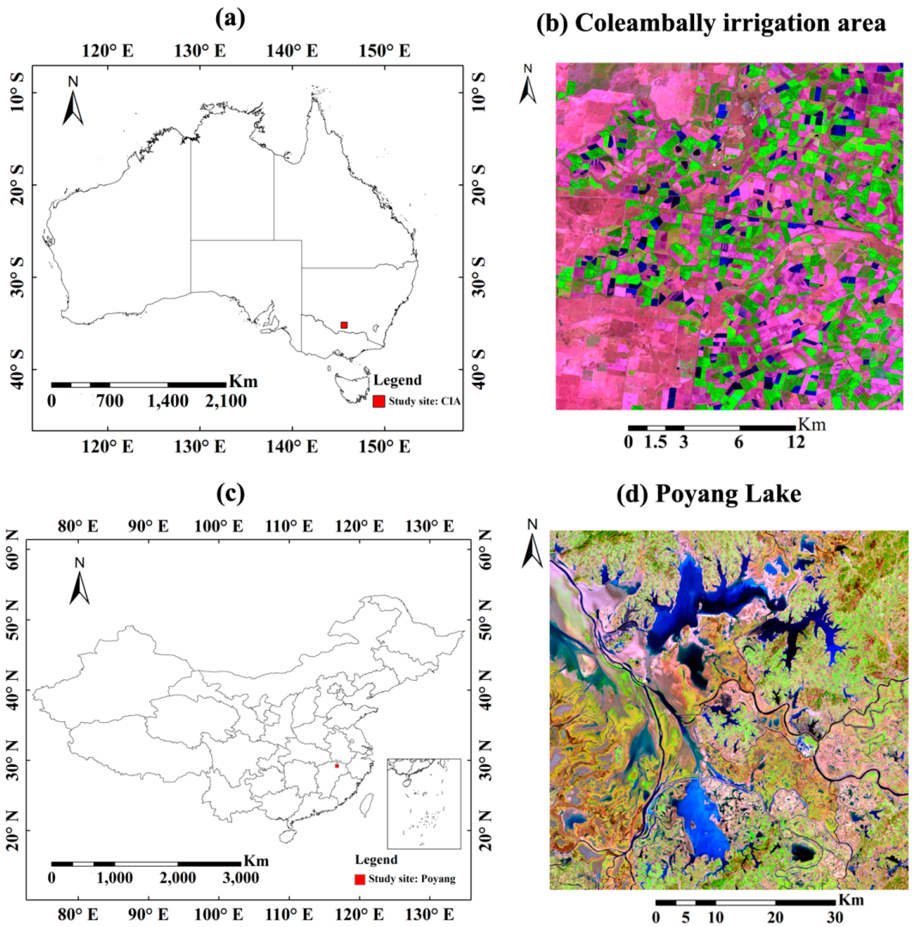
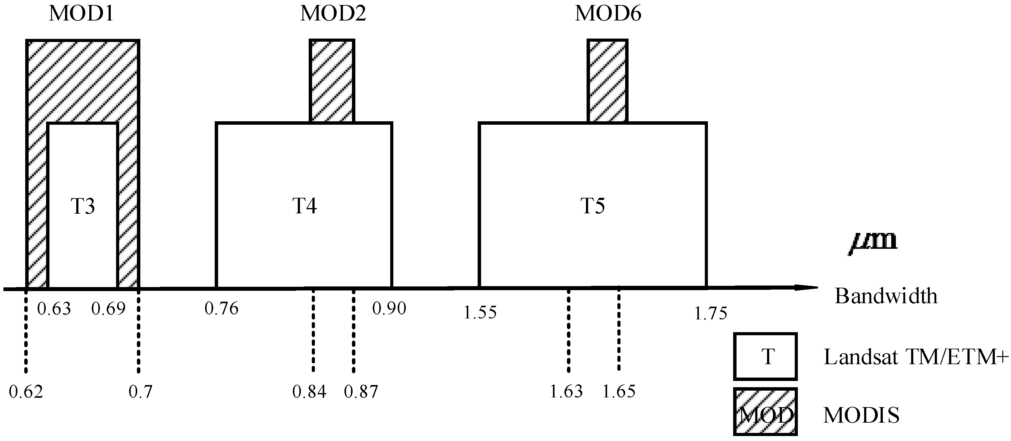
2.1. Study Site Description and Data Preparation

Two study sites were selected in this research (Figure 1). The CIA was chosen as the first validation site. The CIA datasets were provided by the Commonwealth Scientific and Industrial Research Organization, Australia. The CIA is a rice irrigation field located in southern New South Wales, Australia (145°04′E, 34°00′S). The site has been extensively used for time-series remote sensing research [38,39,40,41,42]. We used 17 cloud-free L-M pairs over the CIA during the austral summer growing season in 2001–2002. They are the same time-series L-M datasets as used by Emelyanova et al. [38] and Jarihani et al. [39]. Due to the existing gaps with null values, we selected the main irrigation area of 625 km² (1000 rows by 1000 columns at 25 m resolution). The images were acquired by Landsat-7 ETM+ and atmospherically corrected using MODTRAN4 [43]. The CIA is located entirely in the east-west overlap of two adjacent paths in the Landsat World Reference-2 system (paths/rows 92/84 and 93/84), which allows for an 8-day repeat cycle [38,42]. The corresponding MODIS Terra MOD09GA Collection data were resampled to 25 m resolution using a nearest neighbor algorithm to match the Landsat data resolution after a geometrical transformation. Due to the dimensionality of remotely sensed data [44] and the computation cost of processing all bands, we selected the Landsat red wavelength band (B3), near infrared wavelength band (B4), and mid-infrared I wavelength band (B5). They comprised sufficiently rich information. The corresponding bands for the MODIS imagery were bands 1, 2, and 6.

Poyang Lake, the largest freshwater lake in China, was chosen as the second testing site. It has fluctuating water levels throughout the year. Between March and June, water flows into the lake from five surrounding rivers. It reaches its peak level between July and September, due to the high precipitation in the summer and backflow flood from the Yangtze River. Between October and November, the water subsides, and vast areas covered with wetland vegetation emerge. From December to February, the water level decreases significantly and several small disconnected lakes are visible. To ensure monitoring rapid and significant phenological changes in both the spatial and temporal domains, we specifically chose the southeastern part (116°37′E, 28°33′N) of the water body, because the surface reflectance of the area has been reported to vary significantly throughout the year [45]. Ten cloud-free L-M pairs were available in 2004. The Poyang Lake site covers 3600 km² (2000 rows by 2000 columns at 30 m resolution). All of the Landsat images were acquired by Landsat-5. The digital numbers from the Landsat level 1 product were calibrated and atmospherically corrected using fast line-of-sight atmospheric analysis of hypercubes (FLAASH) [46]. The acquired MODIS daily surface reflectance (MOD09GA) data were reprojected and resampled to the Landsat resolution and extent. As FLAASH uses a similar 6S (Second Simulation of the Satellite Signal in the Solar Spectrum) [47] atmospheric correction approach to the MODIS surface reflectance product, the two sensors’ reflectance were consistent and comparable [7].

Figure 1. Location of the two study sites. (a) A map of Australia with the CIA site labeled in a red square; (b) The RGB composite of the Landsat image with B5, B4, and B3 acquired on 8 October 2001 for the CIA; (c) A map of China with the Poyang Lake site labeled in a red square; (d) The RGB composite of the Landsat image with B5, B4, and B3 acquired on 15 February 2004 for the Poyang Lake wetland.

Dates of the acquired L-M pairs for the Poyang Lake and CIA sites are given in Table 2. For Poyang Lake, less cloud-cover MODIS data on the closest dates were substituted when uncontaminated MODIS images were unavailable on the targeted dates. For the CIA site, the acquired L-M pair dates were well correlated.

Table 2. Dates of the acquired L-M pairs for the Poyang Lake wetland (PLW) and CIA sites. For the Poyang Lake site, less cloud-cover MODIS data on the closest dates were substituted when uncontaminated MODIS images were unavailable on the targeted dates. For the CIA site, the acquired L-M pair dates were well correlated.

**Table 2.** Dates of the acquired L-M pairs for the Poyang Lake wetland (PLW) and CIA sites. For the Poyang Lake site, less cloud-cover MODIS data on the closest dates were substituted when uncontaminated MODIS images were unavailable on the targeted dates. For the CIA site, the acquired L-M pair dates were well correlated.
Image	CIA	Image	PLW
#	Date	#	Date
1	2001/10/08	1	2004/02/15
2	2001/10/17	2	2004/04/19
3	2001/11/02	3	2004/05/05
4	2001/11/09	4	2004/07/24
5	2001/11/25	5	2004/08/09
6	2001/12/04	6	2004/09/26
7	2001/01/05	7	2004/10/12
8	2002/01/12	8	2004/10/28
9	2002/02/13	9	2004/11/29
10	2002/02/22	10	2004/12/15
11	2002/03/10
12	2002/03/17
13	2002/04/02
14	2002/04/11
15	2002/04/18
16	2002/04/27
17	2002/05/04

2.2. Selected Spatiotemporal Fusion Models

We compared three reconstruction-based models, STARFM [2], ESTARFM [15], and improved STARFM (ISTARFM) [48], and one learning-based model, SPSTFM .

2.2.1. STARFM

STARFM [2] needs at least one pair of fine- and coarse-resolution data on the prior or posterior date and one set of coarse-resolution data on the predicted date. It predicts the surface reflectance using a combined weight function, incorporating spectral information from both the fine- and coarse-resolution data. Its implementation is as follows.

(i): One fine-resolution image is used to select candidate similar neighbor pixels using a threshold method. The threshold is determined by the standard deviation of the fine-resolution images and the estimated number of land-cover types.
(ii): Sample filtering is applied to remove poor quality observations from the candidates, which introduces constraint functions to ensure the quality of the selected similar pixels.
(iii): The weights corresponding to each similar pixel are computed with a combined function using the spectral difference, temporal difference, and distance difference.
(iv): The final surface reflectance on the targeted date is predicted with the incorporation of the fine- and coarse-resolution data through the proposed weight function.

2.2.2. ESTARFM

ESTARFM [15] needs at least two pairs of fine- and coarse-resolution data on prior and posterior dates and one coarse-resolution data on the predicted date. It predicts the surface reflectance of the targeted date using a linear combination of spectral information from both the fine- and coarse-resolution data based on the concept of spectral unmixing, incorporating a conversion coefficient and a weight coefficient. Its implementation is as follows.

(i): Similar neighbor pixels are selected from the fine-resolution data on both the prior and posterior dates using the same threshold method as STARFM. The final set of similar pixels is determined by an intersection operation of the results derived from the individual selection in the initial step.
(ii): The weights for all of the similar pixels are determined by the spectral similarity and geographic distance between the targeted pixel and similar pixels.
(iii): The conversion coefficients are computed from the surface reflectance of the fine- and coarse-resolution data during the observation period using a linear regression.
(iv): The two transition images on the targeted date are predicted using the combined function of the fine- and coarse-resolution data and the weight and conversion coefficients.
(v): The final fine-resolution prediction is calculated by incorporating the two transition images in step (iv) through a weight function, which depends on the spectral difference of the coarse-resolution data on the base date and the predicted date.

2.2.3. ISTARFM

ISTARFM [48] provides two prediction modes, in which one or two pairs of base L-M images are used in the blending process. Its implementation is as follows.

(i): Adaptively choose blending modes. ISTARFM first performs a choice for prediction modes according to the number of input L-M pairs within a time-window.
(ii): Similar neighboring pixels are selected from the fine-resolution data through local rules with a logistic constraint function. For one-pair prediction mode, the final similar pixels are retrieved from its individual selection; for multi-pair prediction mode, the final set of similar pixels is retrieved by an intersection operation on the results derived from the individual selection.
(iii): The weights for all similar pixels are determined by four factors: fine-coarse resolution data difference, spectral similarity for fine-resolution data, selective temporal difference and spatial difference.
(iv): The final fine-resolution prediction is calculated by incorporating observed fine- and coarse-resolution data through a weight function in step (iii).

2.2.4. SPSTFM

SPSTFM [29] also requires two pairs of fine- and coarse-resolution data. It predicts fine-resolution reflectance by establishing the correspondence of structures between the fine- and coarse-resolution images via sparse representation. Its implementation is as follows.

(i): High-frequency patches are extracted for dictionary learning. The difference images of the fine- and coarse-resolution data on the prior and posterior dates are extracted for jointly training two dictionaries of high-frequency feature patches.
(ii): Dictionary-pair learning is conducted with the two input difference images using an optimization equation under the theoretical basis of sparse representation and sparse coding. The optimal solution to obtain the best dictionary sets D_l and D_m is K-SVD [49].
(iii): The fine-resolution patches are reconstructed using the enforced same sparse coefficient and the dictionary set D_l, after obtaining the sparse coefficient of the coarse-resolution patch with respect to the dictionary set D_m.
(iv): The fine-resolution reflectance is predicted. Considering the heterogeneity of local changes in actual remote sensing images, the general reconstruction is converted from the image scale to the patch scale using different local weights. The NDVI and normalized difference built-up index (NDBI) are also taken into consideration to measure the change information.

2.3. Comparison Type Setting

As each algorithm needs a different number of base L-M pairs, we divided the prediction patterns into a one L-M pair prediction mode and a two L-M pair prediction mode. Under the given comparison type, we performed blending tests using STARFM (STARFM-One) and ISTARFM (ISTARFM-One) with one L-M pair. All of the models were also used with two L-M pairs (STARFM-Two, ESTARFM, ISTARFM-Two, and SPSTFM). The two prediction modes were conducted on both study sites by producing a Landsat-like image on the targeted date. Specifically, we used one prior closest L-M pair for the one L-M pair prediction, and used one prior and one posterior images that were nearest temporal neighbors to the targeted date for the two L-M pairs prediction. The corresponding actual Landsat observation was also required for validation.

For example, for one L-M pair prediction on the CIA dataset, L-M (10 October 2001) and M (17 October 2001) were used to predict the synthetic Landsat-like data on 12 October 2001, and L-M (17 October 2001) and M (2 November 2001) were used to predict the Landsat-like data on 2 November 2001. For two L-M pair prediction on the CIA dataset, L-M (10 October 2001), L-M (2 November 2001), and M (17 October 2001) were used to predict the synthetic Landsat-like data on 12 October 2001, and L-M (17 October 2001), L-M (9 November 2001), and M (2 November 2001) were used to predict the Landsat-like data on 2 November 2001.

2.4. Quantifying Spatiotemporal Comparability

Due to the compatibility of satellite transit and sensor bandwidth for both onboard Landsat and MODIS, they have similar orbital parameters, such as near-nadir viewing and solar geometries [2,15]. In previous blending applications, there is always an assumption that the Landsat and MODIS data acquired at a given site on the same date will be spatially and temporally comparable after radiometric calibration, geometric referencing, and atmospheric correction [2,7,15]. However, how much the spatiotemporal comparability between the input Landsat and MODIS images affects final prediction accuracy has not yet been addressed. Therefore, we calculated the correlation coefficient of each selected band between the Landsat and MODIS images to denote the spatiotemporal comparability of input L-M pairs.

2.5. Quantifying Landscape Heterogeneity

Study site heterogeneity greatly affects spatiotemporal blending results [2,15]. Characterizing the sensitivity between the landscape heterogeneity and prediction performance requires a robust quantitative metric. We used our newly proposed landscape heterogeneity index (LHI) [40], to quantify the landscape heterogeneity and time-series variances at the two study sites. The newly presented LHI considers the individual pattern of both horizontal and vertical textures of landscape, and employs two threshold strategies to detect whether the neighboring ground pixels differ from each other significantly in both horizontal and vertical directions [40].

2.6. Assessing Prediction Accuracy

The models’ prediction performance was quantitatively evaluated with representative metrics and direct visual inspection. The CC was used to measure correlation between the predicted and actual reflectance. The AAD between the predicted and actual reflectance was calculated to verify the deviation between the simulations and observations. The RMSE and peak signal to noise ratio (PSNR), which are widely used in the quantitative assessment of image quality, were chosen to reflect the overall bias between the simulated and observed reflectance. The Kling-Gupta efficiency (KGE) [50] was used as a compound measure to evaluate the model performance. The KGE accounts for the correlation, variability, and bias, and incorporates these measures into a single multi-objective index. The formula is given below:

KGE = 1 - E D

(1)

E D = \sqrt{{(r - 1)}^{2} + {(α - 1)}^{2} + {(β - 1)}^{2}}

(2)

α = σ_{p} / σ_{o}

(3)

β = μ_{p} / μ_{o}

(4)

where ED denotes the Euclidian distance from the ideal point, r is the CC between the predicted and observed reflectance, α and β denote a ratio of the relative deviation and mean variability of the predicted and observed reflectance, σ_p and σ_o denote the standard deviation of the predicted and observed reflectance, respectively, and μ_p and μ_o denote the mean value of the predicted and observed reflectance, respectively. Thus, the ideal KGE equals 1.

The performance for each prediction mode was compared. Selected comparisons between the prediction modes were also made to validate how the number of L-M pairs affected the prediction results.

3. Results

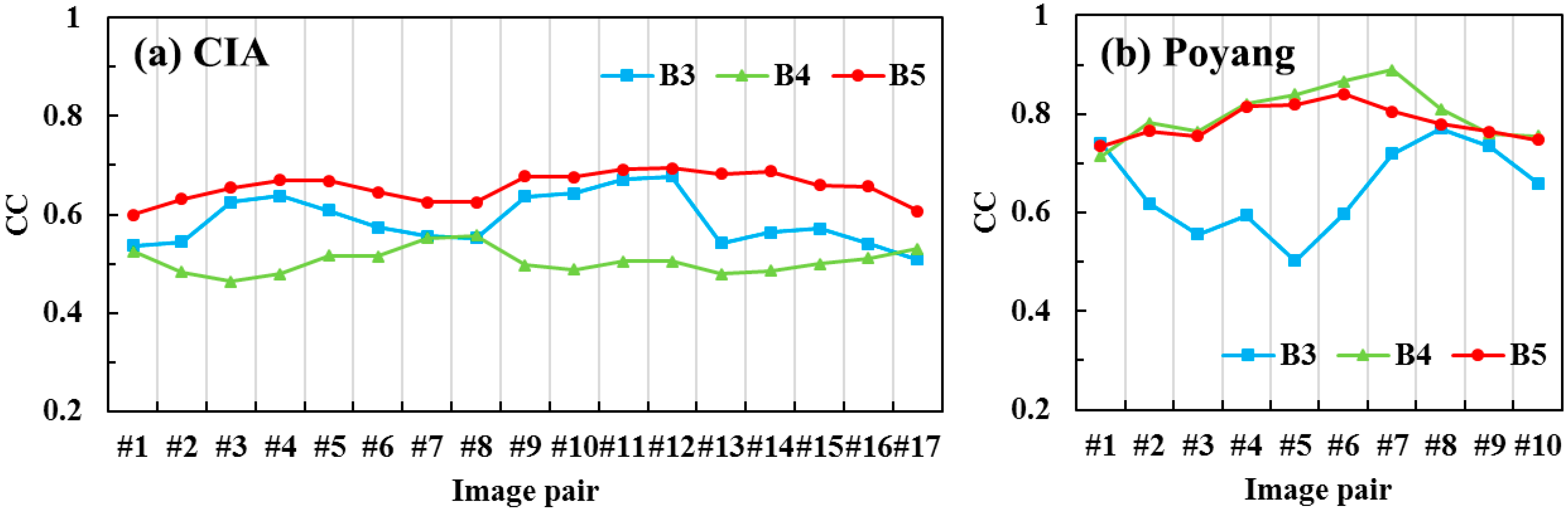
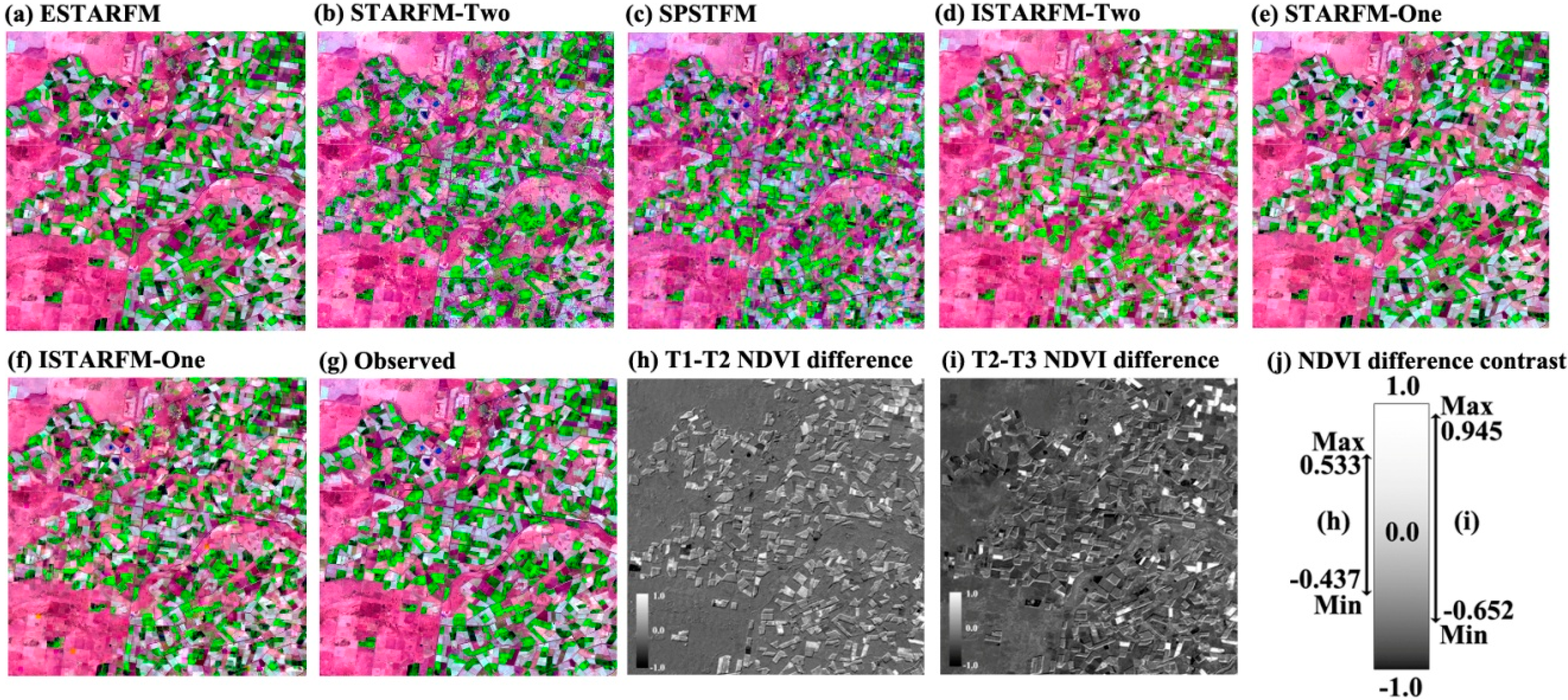
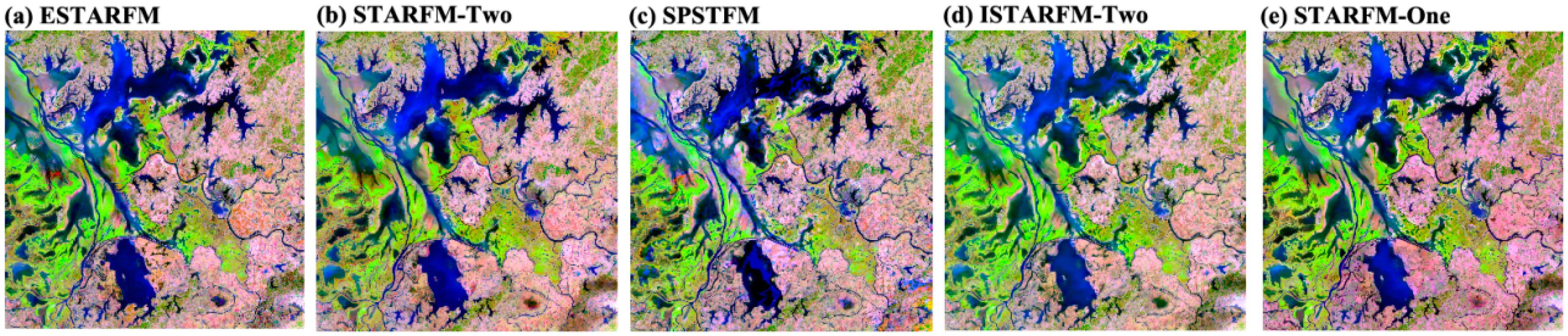
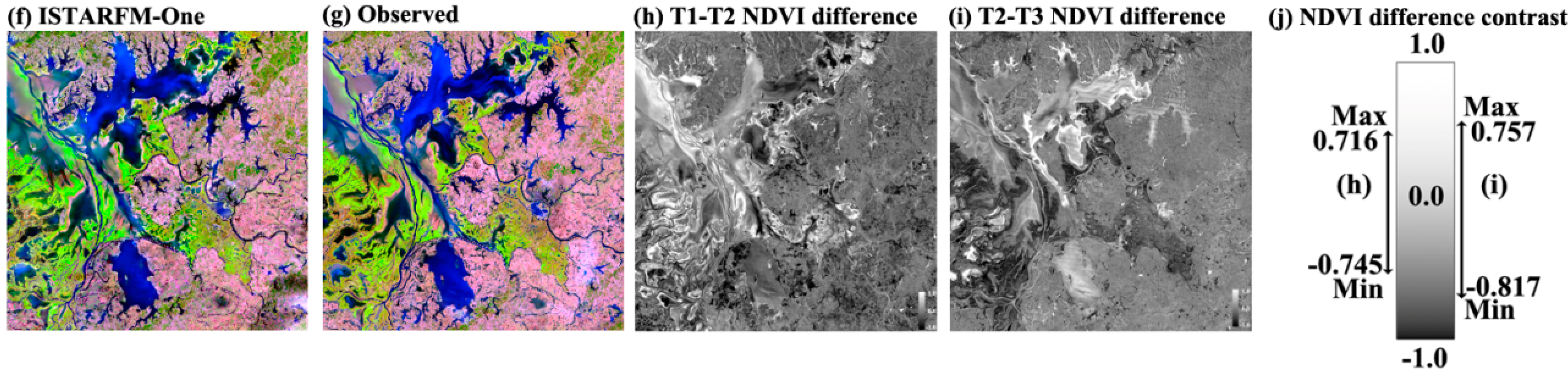
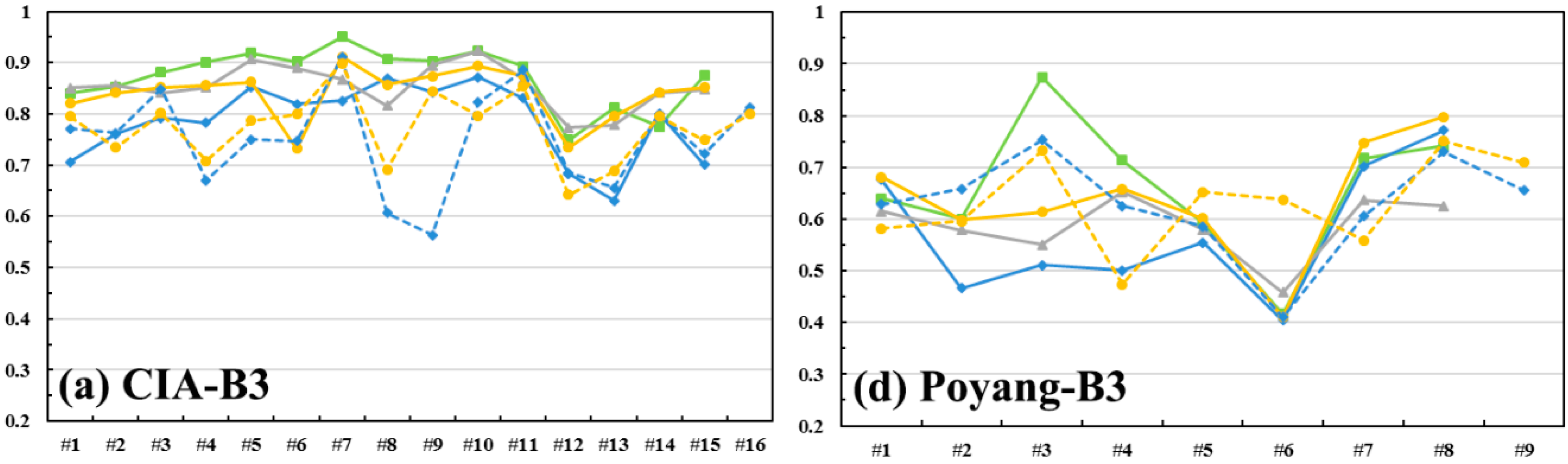
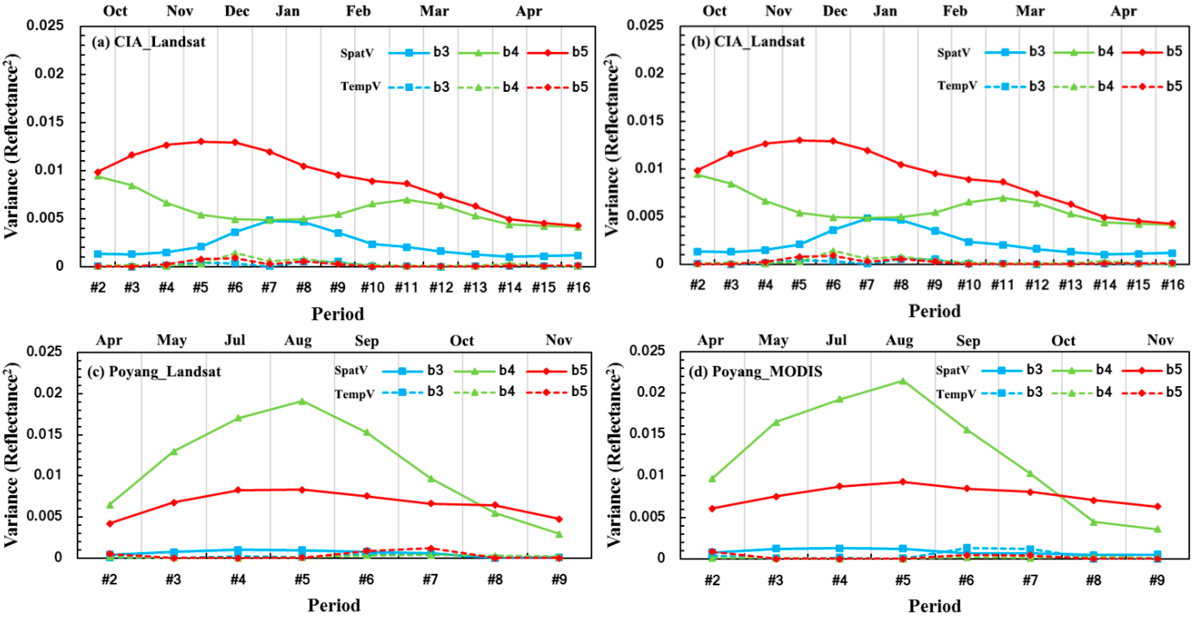
3.1. Spatiotemporal Comparability

The spatiotemporal comparability of L-M pairs acquired on each available date for both the CIA and Poyang Lake site is shown in Figure 2.

Figure 2. The CC values of the corresponding L-M pairs acquired on the same date for both the CIA and Poyang Lake sites. (a) The general variance of the CC at the CIA site, ranging from 0.50–0.68 for B3, 0.46–0.56 for B4, and 0.59–0.70 for B5; (b) The general variance of the CC at the Poyang Lake site. The CC varies from 0.50–0.77 for B3, 0.71–0.89 for B4, and 0.73–0.85 for B5.

Figure 3. The position contrast of the selected Landsat TM/ETM+ and MODIS bands in the electromagnetic spectrum.

Figure 2a reveals that the spatiotemporal comparability of B3 (red) and B5 (MIR I) of the L-M pairs were better than that of B4 (NIR), and Figure 2b shows that B4 and B5 were more comparable than B3. However, the position contrast of selected bands in Figure 3 shows that B3 has the highest level of overlapped bandwidth with respect to its corresponding L-M bands, B4 has the second highest, and B5 has the lowest. Besides the geometric difference mentioned in Section 2.4, the critical factor that impacts spatiotemporal comparability is the spectral response associated with various landscapes. Since the CIA is a rice irrigation field and B4 is most sensitive to green vegetation, the high variance of surface reflectance in B4 results in its lower comparability than the other two bands in the CIA site. Due to the vast water body that is predominant in the Poyang Lake site, the surface reflectance of water in the near-infrared and mid-infrared band is much lower than that in the visible bands. Moreover, the chlorophyll content in the aquaria environment results in more variability of reflectance in the visible bands.

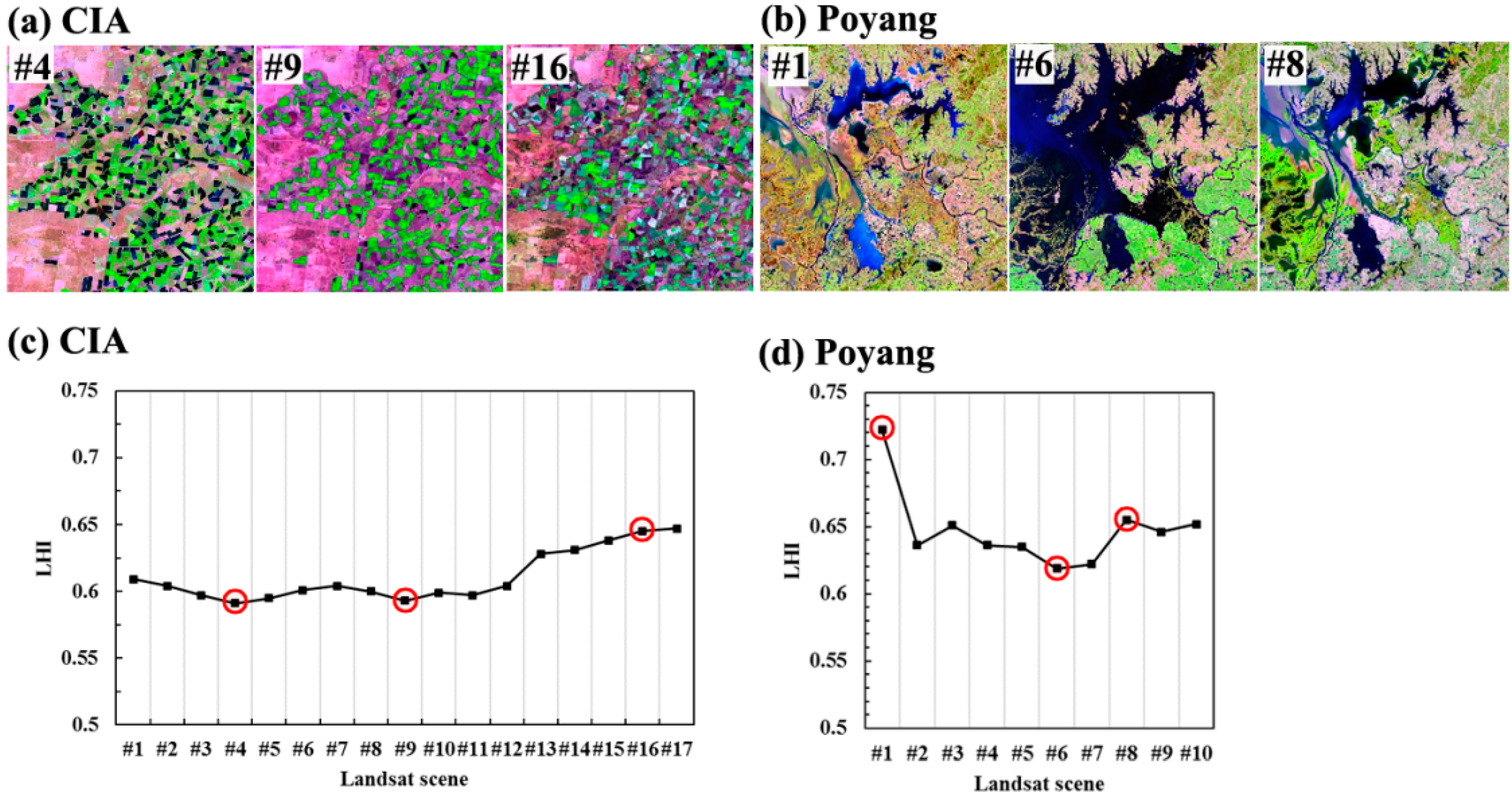
3.2. Landscape Heterogeneity Changes

Figure 4 shows that the selected ETM+ scenes corresponded to significant changes in the landscape heterogeneity for both sites. For example, significant seasonal phenology changes at the CIA site occurred from 9 November 2001 to 13 February 2002, but the overall landscape distribution was stable. From 13 February to 27 April 2002, we can clearly see that the land cover changed and became more heterogeneous, being consistent with the computed LHI changes. The changes in the water area at the Poyang Lake site dominated the landscape heterogeneity variance.

Figure 4. Selected Landsat scenes and time-series plots of landscape heterogeneity changes using the LHI. (a) ETM+ scenes of the CIA site acquired on 9 November 2001 (#4), 13 February 2002 (#9), and 27 April 2002 (#16); (b) TM scenes of the Poyang Lake site acquired on 15 February 2004 (#1), 26 September 2004 (#6), and 28 October 2004 (#8); (c,d) Time-series plots of the landscape heterogeneity using the LHI, indicating with red circles the specific images in (a,b), for the CIA site (c) and the Poyang Lake site (d).

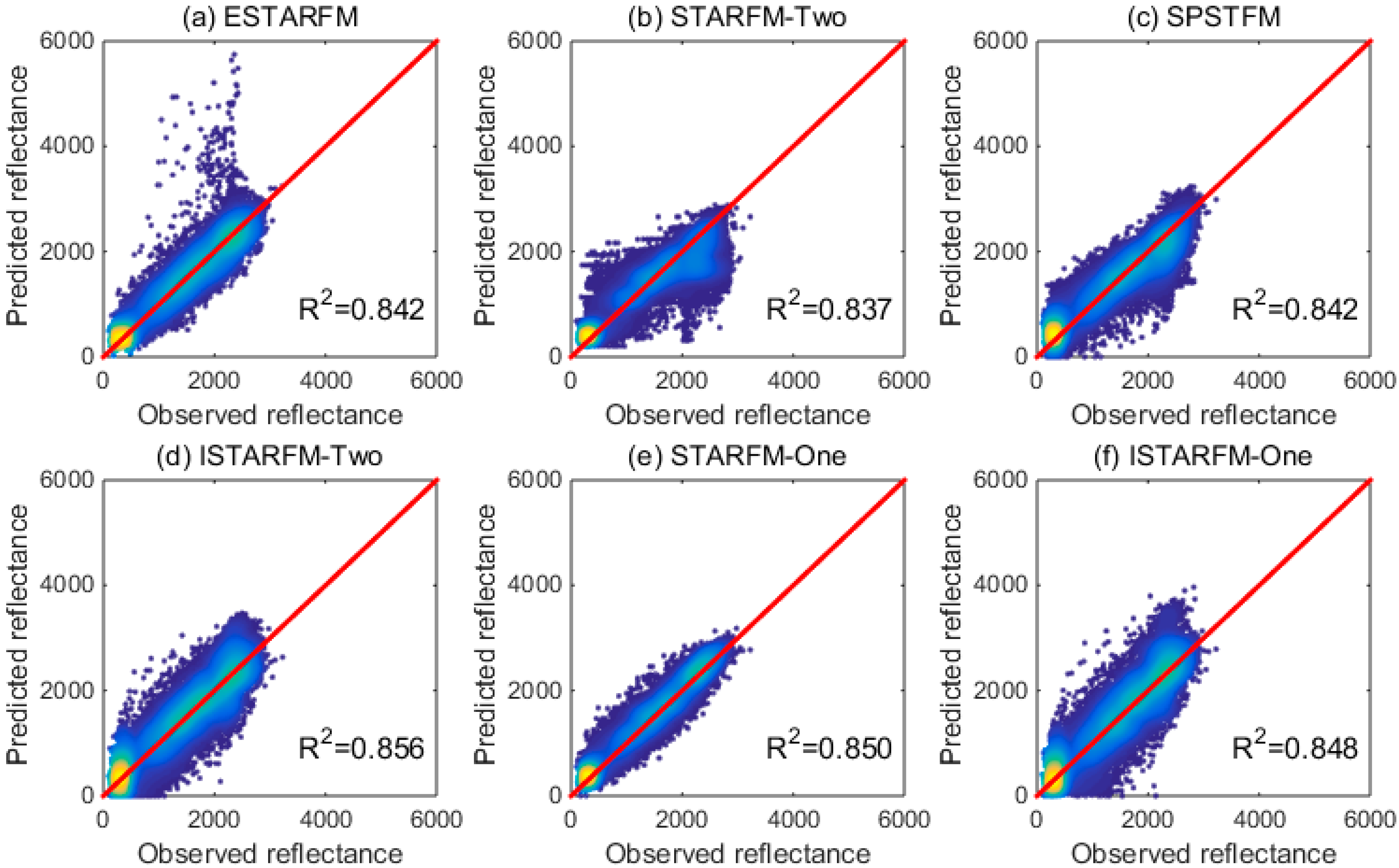
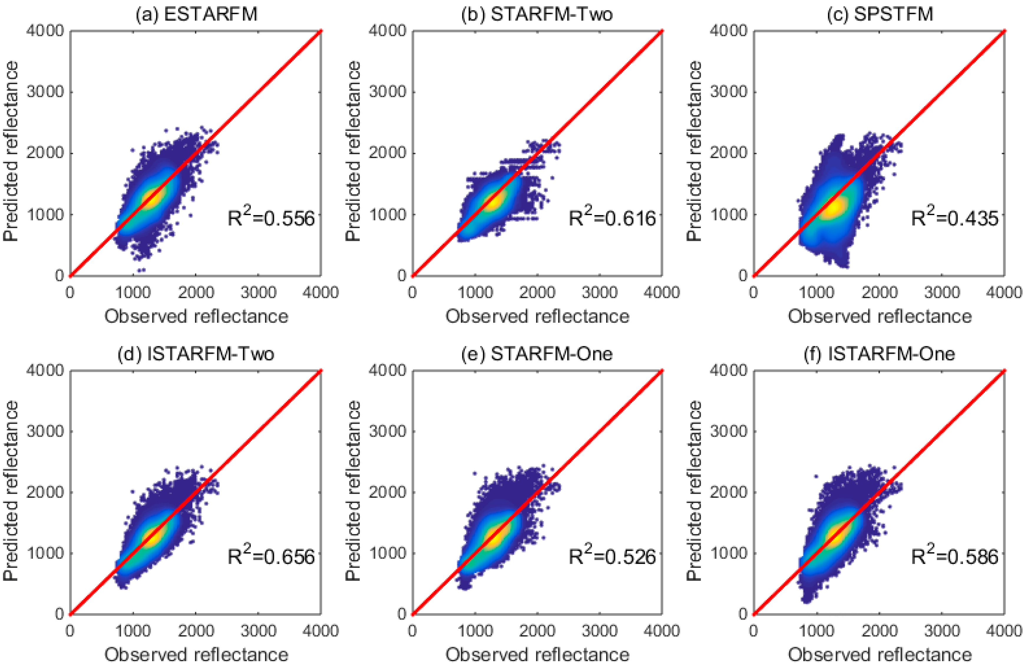
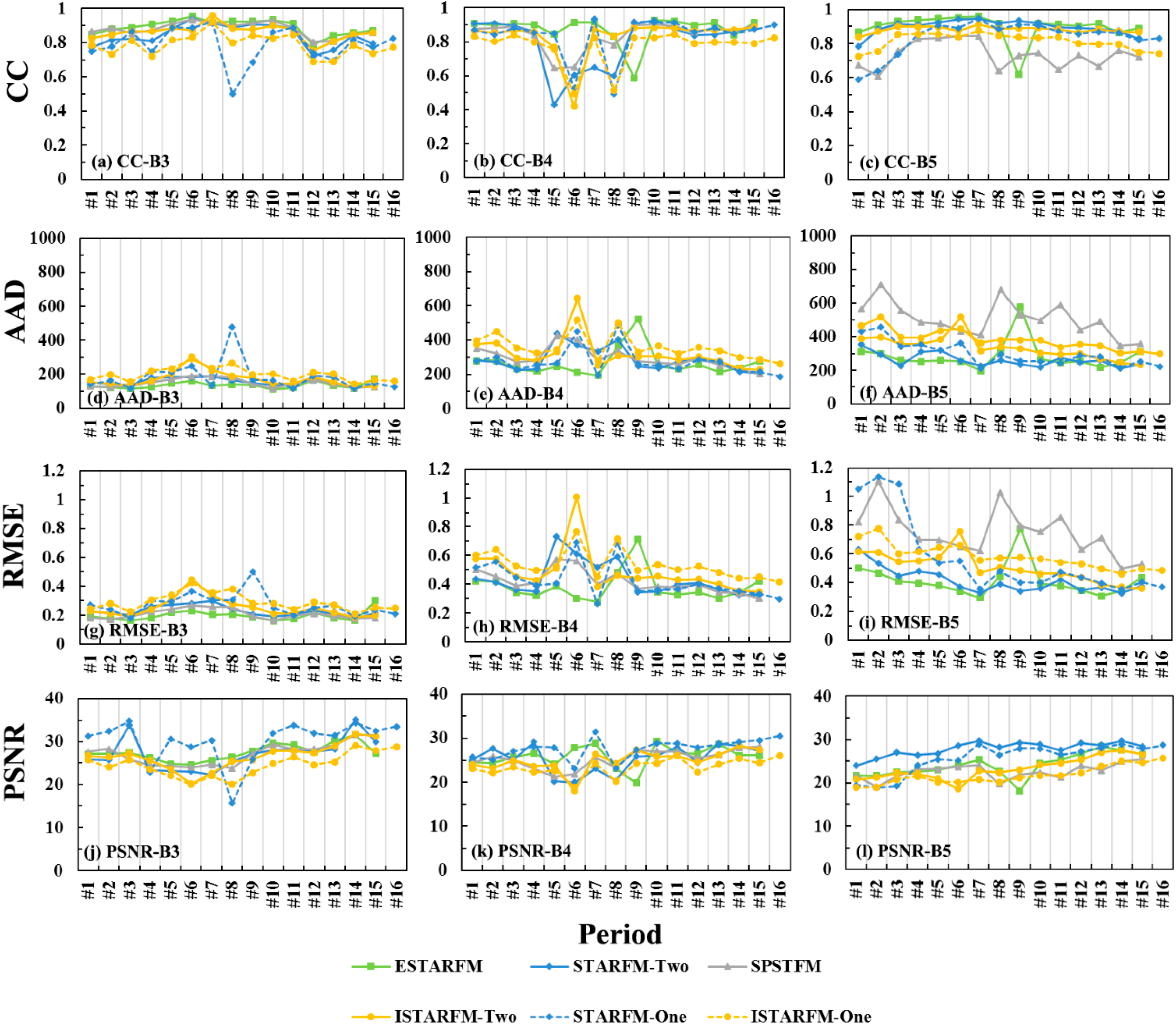
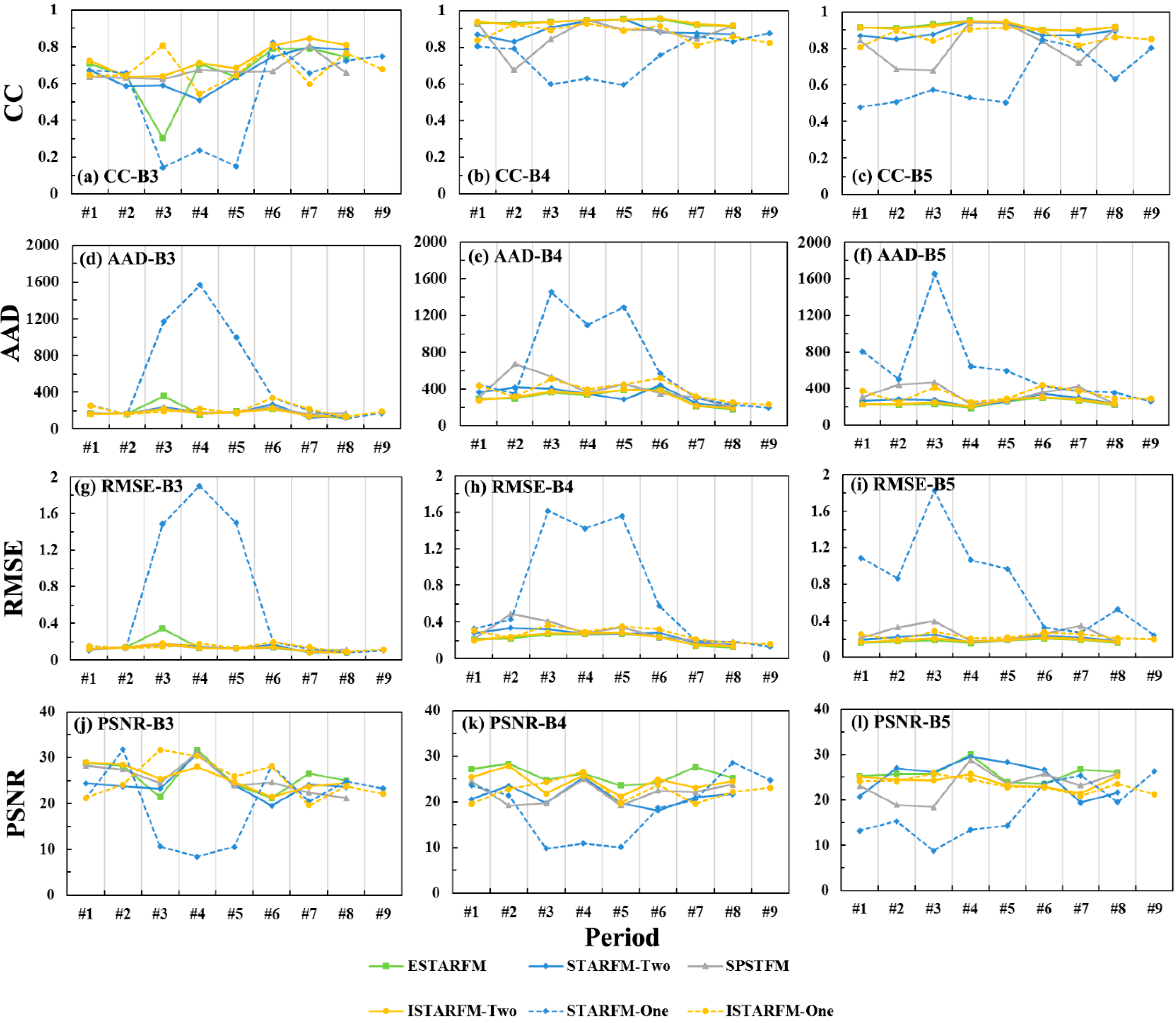
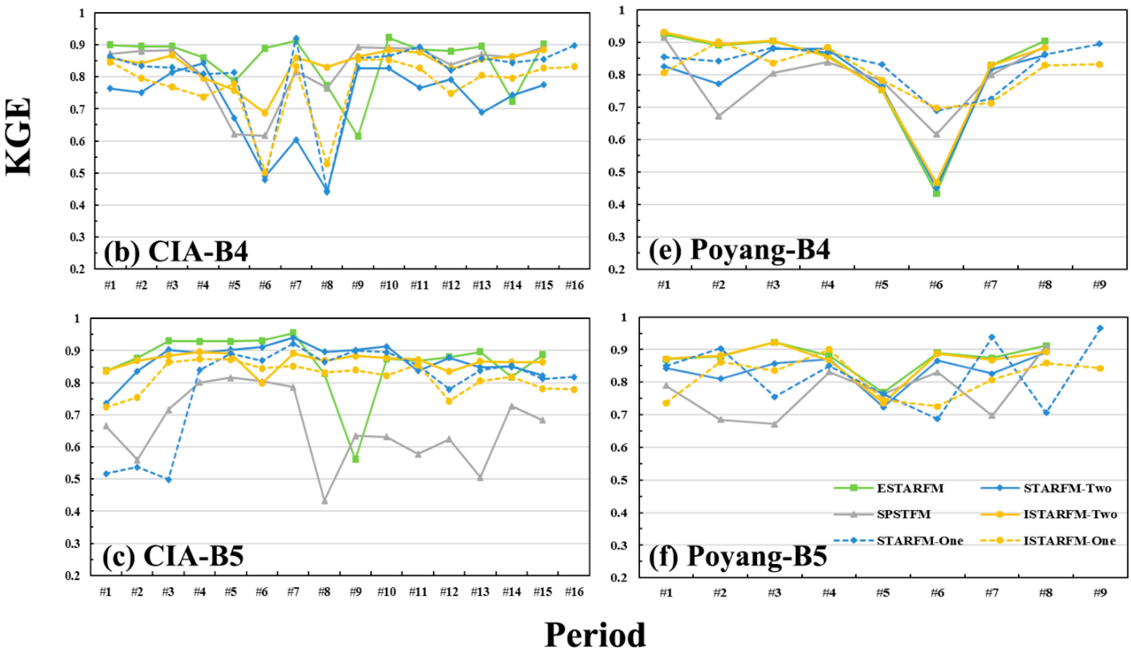
3.3. Prediction Performance

Figure 5 and Figure 6 show actual Landsat observations and predicted Landsat-like images using the four blending models under the two prediction modes on 12 January 2002 and 29 November 2004 for the CIA and Poyang Lake sites, respectively. The NDVI difference images between the prior and predicted dates, and between the predicted and posterior dates, at the Landsat resolution were also shown in Figure 5 and Figure 6. A visual comparison of each prediction and its corresponding observed Landsat data could be made. All of the predictions (Figure 5a–f and Figure 6a–f) using the selected blending models captured the general changing information during the prediction period seen in the actual observations (Figure 5g and Figure 6g). This demonstrates the possibility and utility of these spatiotemporal blending applications.

Figure 5. Predicted Landsat-like images and the observed Landsat ETM+ image for the CIA site on 12 January 2002. (a–d) Blended images under the two L-M pairs prediction mode using ESTARFM, STARFM-Two, SPSTFM, and ISTARFM-Two, respectively; (e,f) Blended images under the one L-M pair prediction mode using STARFM-One and ISTARFM-One; (g) Observed ETM+ image; The NDVI difference images (h) between the prior (T1) and predicted (T2) date, and (i) between the predicted (T2) and posterior (T3) dates, respectively, in which darker regions represent smaller changes and lighter regions denote larger changes. (j)The NDVI difference contrast of (h) and (i).

Figure 6. Predicted Landsat-like images and the observed Landsat TM image for the Poyang Lake site on 29 November 2004. Similarly, (a–d) Blended images under the two L-M pairs prediction mode; (e,f) Blended images under the one L-M pair prediction mode. (g) Observed ETM+ image; The NDVI difference image (h) between the prior and predicted dates, and (i) between the predicted (T2) and posterior (T3) dates, respectively; (j) The NDVI difference contrast of (h) and (i).

Figure 7 and Figure 8 show the sample red band (B3) to validate the l-to-l line correlation between the observed and estimated reflectance. At the CIA site (Figure 7), ESTARFM clearly overestimates and STARFM-Two underestimates. The remaining blending models produce better 1-to-1 line correlations. At the Poyang Lake site (Figure 8), a group of ESTARFM predicted pixels are under-estimated and the estimated reflectance using SPSTFM produces a large bias. A visual inspection of this randomly selected date at each site indicates that ISTARFM-One and -Two performed more stably.

Figure 7. Comparison of the observed and predicted reflectance on 12 January 2002 for the red band (B3) from each blending model (a–f) using 1-to-1 fitting line at the CIA site. The scale factor of reflectance is 10,000, which was also used for the quantitative assessment.

Figure 8. Comparison of the observed and predicted reflectance on 29 November 2004 for the red band (B3) from each blending model (a–f) using 1-to-1 fitting line at the Poyang Lake site. The scale factor of reflectance is 10,000, which was also used for the quantitative assessment.

3.4. Accuracy Assessment

Many previous blending studies have performed accuracy assessments using tables and scatter plots of actual observations versus predicted Landsat-like data, such as those in Figure 7 and Figure 8. We made time-series predictions for the three selected bands at two sites under two prediction modes. This produces 426 possible sets of assessment: 276 for the two L-M pair prediction mode (180 for the CIA site and 96 for the Poyang Lake site) and 150 for the one L-M pair prediction mode (96 for the CIA site and 54 for the Poyang Lake site). We employed a “curve” visualization to compare the prediction accuracy of selected bands of different fusion models on time-series date sequences. The spatiotemporal fusion models under the two L-M pair prediction mode were depicted using solid lines with different colors, while the models under the one L-M pair prediction mode were denoted using dashed lines. Each assessment measure shown in separated rows, i.e., CC, AAD, RMSE, and PSNR, was displayed up to bottom, respectively. The larger CC and PSNR denote higher correlations between the observed and predicted reflectance. The smaller AAD and RMSE denote minor bias. Therefore, the four measures can be considered at the same time.

Figure 9 depicts time-series changes of selected measures with respect to the four blending models for the CIA site. The CC curve chart (Figure 9a–c) shows the relative stability and superiority of ESTARFM and ISTARFM-Two over the other models. We can draw the same conclusion from the AAD curve chart (Figure 9d–f); however, larger biases can be seen for SPSTFM and ISTARFM-One, especially for the short-wave near-infrared band (B5).

Figure 9. “Curve” visualization of the individual accuracy measures of the time-series predictions for the CIA site, showing the accuracy measures: CC (a–c); AAD (d–f); RMSE (g–i); and PSNR (j–l).

Correspondingly, Figure 10 depicts time-series changes of the selected measures with respect to the four blending models for the Poyang Lake site. The four types of curve charts (Figure 10) show that ISTARFM-Two outperforms the other models, and ESTARFM ranks at the second place. However, larger biases can be seen for STARFM-One during the period from date #3 to #5 from the curve chart (Figure 10). SPSTFM also produces large biases during the period from date #3 to #4.

Figure 11a–c (the left column) depict the time-series variability of the KGE for B3, B4, and B5 at the CIA site, respectively, and Figure 11d–f (the right column) represent the KGE variability of the same bands at the Poyang Lake site, respectively. It has shown that one model may yield different accuracy for individual band. The ISTARFM-Two and ESTARFM perform more stably for blending.

Figure 10. “Curve” visualization of individual accuracy measures of the time-series predictions for the Poyang Lake site, showing the accuracy measures: CC (a–c); AAD (d–f); RMSE (g–i); and PSNR (j–l).

Figure 11. KGE values calculated for each model for the three selected bands at (a–c) the CIA and (d–f) Poyang Lake sites.

4. Discussion

4.1. Selected Blending Models Performance

The objective of this research was to evaluate spatiotemporal blending models under two prediction modes using L-M data at the CIA and Poyang Lake sites. The selected blending models had minimum input requirements and no ancillary data were used, such as land-cover classification result or phenology timetables.

More input L-M pairs did not always ensure higher prediction accuracy because the phenology predicted for the Poyang Lake site using only one prior L-M pair was closer to the actual observations than that using two L-M pairs, based on both visual and quantitative comparisons. We took the blending model using two L-M pairs as an example, assuming that L_pm and L_pn represent the transient Landsat-like data at the date t_p, predicted from the input L-M pair at t_m and t_n, respectively. The synthetic prediction of the Landsat-like data at t_p can be obtained by the compound weighting function:

L_{p} = W_{m} \cdot L_{p m} + W_{n} \cdot L_{p n} = W_{m} \cdot L_{p m} + (1 - W_{m}) \cdot L_{p n}

(5)

Consequently, the range of L_p should satisfy

min {L_{p m}, L_{p n}} < L_{p} < max {L_{p m}, L_{p n}}

(6)

where

W_{m}

and

W_{n}

denote the weights of the transient predictions

L_{p m}

and

L_{p n}

, respectively

min {\cdot}

and

max {\cdot}

denote the minimizing and maximizing operations. However, when one transient prediction shows a large bias due to a large spectral contrast between the base and predicted dates, the final prediction deviation will be large, according to Equation (5). Therefore, we could use the idea proposed in [48] that L-M pair pre-selection based on the CC of coarse-resolution data between the base and predicted dates should be performed when more than two L-M pairs exist.

For this purpose, we tested STARFM-One and ESTARFM on the CIA site, with base dates preselected using fewer MODIS images for the predicted date. For the STARFM-One, we used MODIS image on 9 November 2001 (#4) and base L-M pairs on 8 October 2001 (#1), 17 October 2001 (#2), and 2 November 2001 (#3), respectively, to produce a synthetic Landsat-like image on 9 November 2001 (#4). For the ESTARFM, we fixed the prior L-M pair on 2 November 2001 (#3), and used posterior L-M pairs on 25 November 2001 (#5), 4 December 2001 (#6), 5 January 2002 (#7), 12 January 2002 (#8), and 13 February 2002 (#9), respectively, to produce a synthetic Landsat-like image on 9 November 2001 (#4).

Table 3 shows that the CC between the base date and predicted date image with the order from small to large is #1, #2, and #3 for the STARFM-One model test. For the ESTARFM model test, the corresponding order is #7, #8, #6, and #5. With a comparison between Table 3 and the quantitative assessment results (Table 4 and Table 5), it reveals that the model performance is consistent with the CC value of MODIS images between the base and predicted dates. Taking STARFM-One with B3 for instance, the CC value increases from 0.42 to 0.58, and reaches 0.79, while the KGE criteria between the predicted and observed reflectance correspondingly increases from 0.50 to 0.65, and reaches 0.86. The same conclusion can be verified from another measure (i.e., CC). For the ESTARFM model test, with the CC decreased from 0.76 to 0.39 with B3, 0.75 to 0.10 with B4, and 0.89 to 0.73 with B5, its model performance saw a slight decrease rather than producing large bias.

Table 3. The correlation coefficient (CC) of MODIS images between the base and predicted dates in the CIA site. For example, “#1~#4” denotes the CC value between the prior MODIS image on 8 October 2001 (#1) and the MODIS image on 9 November 2001 (#4).

**Table 3.** The correlation coefficient (CC) of MODIS images between the base and predicted dates in the CIA site. For example, “#1~#4” denotes the CC value between the prior MODIS image on 8 October 2001 (#1) and the MODIS image on 9 November 2001 (#4).
	B3	B4	B5
Mode	B3	B4	B5
#1~#4	0.42	0.52	0.60
#2~#4	0.58	0.56	0.74
#3~#4	0.79	0.62	0.83
#4~#5	0.76	0.75	0.89
#4~#6	0.59	0.53	0.79
#4~#7	0.39	0.14	0.73
#4~#8	0.40	0.10	0.74

Table 4. The quantitative assessment of STARFM-One prediction performance using different prior input L-M pairs in the CIA site. For example, “#1~#4” denotes the prediction mode in which the L-M pair on 8 October 2001 (#1) and MODIS image on 9 November 2001 (#4) are used to predict Landsat-like fusion on 9 November 2001 (#4).

**Table 4.** The quantitative assessment of STARFM-One prediction performance using different prior input L-M pairs in the CIA site. For example, “#1~#4” denotes the prediction mode in which the L-M pair on 8 October 2001 (#1) and MODIS image on 9 November 2001 (#4) are used to predict Landsat-like fusion on 9 November 2001 (#4).
	Criteria	KGE			CC
Mode	Band	B3	B4	B5	B3	B4	B5
#1~#4		0.50	0.71	0.42	0.50	0.76	0.47
#2~#4		0.65	0.72	0.51	0.65	0.80	0.61
#3~#4		0.86	0.81	0.50	0.86	0.88	0.73

Consequently, the CC value of coarse-resolution data between base and predicted dates should be an important reference for selecting input L-M pairs when more than two L-M pairs exist, especially for the STARFM model.

Table 5. The quantitative assessment of ESTARFM prediction performance using different prior input L-M pairs at the CIA site. For example, “#3~#4~#5” denotes the prediction mode in which the L-M pairs on 2 November 2001 (#3) and 25 November 2001 (#5) and MODIS image on 9 November 2001 (#4) are used to predict Landsat-like fusion on 9 November 2001 (#4).

**Table 5.** The quantitative assessment of ESTARFM prediction performance using different prior input L-M pairs at the CIA site. For example, “#3~#4~#5” denotes the prediction mode in which the L-M pairs on 2 November 2001 (#3) and 25 November 2001 (#5) and MODIS image on 9 November 2001 (#4) are used to predict Landsat-like fusion on 9 November 2001 (#4).
	Criteria	KGE			CC
Mode	Band	B3	B4	B5	B3	B4	B5
#3~#4~#5		0.87	0.90	0.92	0.88	0.90	0.92
#3~#4~#6		0.85	0.88	0.91	0.86	0.88	0.91
#3~#4~#7		0.83	0.85	0.91	0.85	0.86	0.91
#3~#4~#8		0.84	0.85	0.90	0.85	0.85	0.91

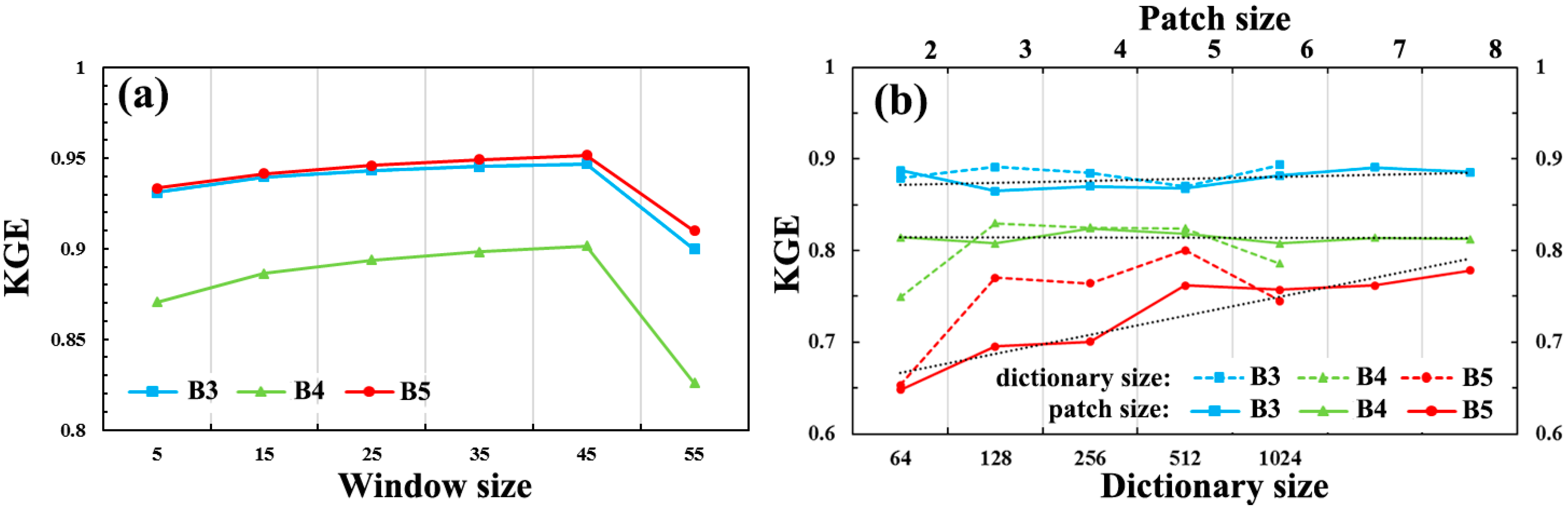
4.2. Model Parameter Selection

Spatiotemporal blending results are sensitive to prerequisites from both input data and parameter setting. Two major types of parameter differences were considered in our study: (i) the spatiotemporal comparability of the input L-M pairs, the landscape heterogeneity and the spatiotemporal variances of study sites; and (ii) preset parameters, such as the moving window size for reconstruction-based methods and the dictionary/patch size for learning-based methods.

The spatiotemporal comparability of the L-M pair on the same date may not be the critical factor impacting prediction accuracy. Figure 2b (Poyang Lake) shows overall higher spatiotemporal comparability than Figure 2a (CIA). However, the KGE criteria in Figure 11 show that overall prediction accuracy at the Poyang Lake site (the right column) is not obviously higher than that at the CIA site (the left column), even though the KGE value with B3 at the Poyang Lake site (Figure 11b) is lower than that at the CIA site. On the other hand, for the same study site, spatiotemporal comparability should also be regarded as an optional reference. As mentioned in Section 3.1, B4 and B5 are more comparable than B3 at the Poyang Lake site from Figure 2b. It is interesting to note that the KGE result with respect to the Poyang Lake site shows that B3 produces larger bias than the other two bands. Based on this aspect, spatiotemporal comparability seems to have the utility to account for prediction accuracy difference regarding band spectrums.

Landscape heterogeneity can also affect the predicted Landsat-like image produced. Figure 3c shows a significant increase in the LHI for the CIA site from 10 March 2002 (#11), which corresponded to a decrease in the prediction accuracy of all of the blending models in Figure 9a–c. However, by comparing the LHI and KGE measures, we could conclude that ESTARFM was superior to the other blending models, due to the use of the conversion coefficient. Quantitatively, ESTARFM produced acceptable predictions when the LHI was below 0.65.

Spatial and temporal variances for landscape are strongly associated with performance of the spatiotemporal fusion model [38,39]. Similar to the procedure performed by Emelyanova et al. [38], we partitioned the overall variance of the L-M datasets for the CIA and Poyang Lake sites into individual spatial and temporal variances using the approach proposed by Sun et al. [51], aiming to analyze all models’ performance based on the spatial and temporal variances.

The curves in Figure 12 show that the spatial and temporal variances at both the Landsat and MODIS resolutions have consistent changing trends. Greater spatiotemporal variance at the Landsat resolution than at the MODIS resolution was witnessed. Obvious differences between the bands can be seen in Figure 12, mainly due to the different spectral response associated with different landscape. The spatial variance of B5 at the CIA site was largest throughout the study period, due to the sharp spectral contrast between the irrigated fields and the fallow fields, dry land pastures, and woodlands [38]. Between acquisition dates 2 and 6, the spatial variance of B5 was relatively high, whereas the spatial variance of B3 decreased. All three bands had low temporal variance at the CIA site, except for an obvious fluctuation between acquisition dates 3 and 7. The spatial variance of B4 at the Poyang Lake site was largest due to the spectral response of the water areas and the subsequent vegetation growth. The fluctuating water levels throughout the year resulted in a large spatial rather than temporal variance. Particularly between acquisition dates 2 and 5, the spatial variance of B4 and B5 stayed high, whereas the temporal variance stayed low.

The partitioned spatial variance was larger than the temporal variance at both the CIA and Poyang sites, especially for the Poyang Lake site that the spatial variance was highly dominant due to its fluctuating water level throughout the year. The quantitative measures showed that ESTARFM produced smaller errors than STARFM-Two at most dates for both sites. It supported the conclusion reached by Emelyanova et al. [38] that ESTARM was superior when spatial variance was dominant. As ISTARFM was developed based on the STAFRM-like framework, it worked better when temporal variances was dominant. However, ISTARFM could perform better than STARFM in predicting situation where significant spatial variance occurred, for its combination with a time-window and pre-selection of input L-M pairs [48]. SPSTFM does not seem to be sensitive to land cover spatiotemporal variance, since its prediction framework was based on dictionary learning. From the KGE assessment results in Figure 11, ESTARFM and ISTARFM-Two produced relatively more stable blending accuracies than the other models. One model could also produce different blending accuracies for each band, due to the different spectral responses to the ground surface.

A comparison of selected blending models should be performed under a unified framework, especially when setting autologous model parameters such as the moving window size of reconstruction-based methods. The larger the moving window size, the more spectral and texture information from neighboring pixels will be introduced into the estimated reflectance of the central pixel. The computation will also increase exponentially. We selected three L-M pairs (#7, #8, and #9 in Table 2) from the CIA site as a case study to validate these parameters. The effect of the moving window size on predictions was analyzed with respect to ESTARFM. The size was sampled from 5 × 5, 15 × 15, …, 55 × 55. The dictionary and patch size are also trade-off factors for learning-based methods. The patch size directly affects the spectral and texture information contained in each sampled patch. We tested the patch size using seven patch sizes (2 × 2, 3 × 3, …, 8 × 8), holding the dictionary size at 512. We then analyzed how the dictionary size affected the blending accuracy by testing five dictionary sizes (64, 128, 256, 512, and 1024), holding the patch size at 4 × 4. We evaluated the KGE and computation cost in both tests, and a Windows PC with 3.40-GHz Intel Core 5 CPU and 8 GB RAM was employed as processor in this study.

Figure 12. At the CIA (a,b) and Poyang Lake sites (c,d), changes in the spatial (SpatV) and temporal (TempV) variance over time at the Landsat (a,c); and MODIS (b,d) resolutions.

Figure 13. Model parameters affect the KGE. (a) Changes in the KGE of the three key bands as the moving window size increases; (b) Changes in the KGE of two bands as the dictionary (bottom axis) and patch (upper axis) sizes increase.

Figure 13a shows that ESTARFM produced a better KGE as the window size increased with an interval step of 10. The KGE then decreased after reaching its maximum. Figure 13b shows that the performance of SPSTFM with B3 and B4 was kept stable as the patch size increased while the SPSTFM performance with B5 improved as patch size increased. The model performance first improved as the dictionary size increased, then fluctuated. The increase in the parameter sizes led to an increase in the computation time, especially for the moving window size and dictionary size (Table 6). However, the larger computation costs with larger window size and dictionary size did not ensure a continuous increase in the prediction accuracy. The trade-off between accuracy and computation and optimal parameter setting for blending models are two key areas for any spatiotemporal fusion procedure.

Table 6. Changes in the computation cost as the model parameters change.

**Table 6.** Changes in the computation cost as the model parameters change.
Window Size	Time Cost	Patch Size	Time Cost	Dictionary Size	Time Cost
5	8 m 59.58 s	2	4 m 26.96 s	64	2 m 14.53 s
15	11 m 19.39 s	3	4 m 29.25 s	128	2 m 33.83 s
25	15 m 50.02 s	4	4 m 30.42 s	256	3 m 10.12 s
35	21 m 47.90 s	5	4 m 30.68 s	512	4 m 30.42 s
45	29 m 52.33 s	6	4 m 32.21 s	1024	7 m 30.40 s
55	39 m 8.80 s	7	4 m 50.66 s
		8	4 m 50.90 s

4.3. Problems with Existing Blending Models

Transformation-based methods mainly focus on the integration of spatial and spectral information for image enhancement. However, they do not construct a distinct blending relationship between spatial and temporal information. Acerbi-Junior et al. [20] attempted to enhance the spatial resolution of MODIS with Landsat data using a wavelet transformation. They performed the spatiotemporal information enhancement of the L-M data on the base date and could not predict the synthetic Landsat-like data on a targeted date. However, when considering multi-information fusion including spectral details, the transformation-based method is recommended, either alone or combined with other blending frameworks.

Reconstruction-based methods have gained notice since the proposal of STARFM. The spatial and temporal adaptive fusion framework provides us with an excellent fusion approach for blending data that have a high spatial resolution but low temporal resolution with data that have a high temporal resolution but low spatial resolution. It has proven useful in dynamic monitoring and phenology disturbance detection over short periods or not significantly changeable landscapes. The biggest obstacle for the development of reconstruction-based methods is how to deal with the assumption that “the land cover type and sensor calibration do not change between the prior and predicted date” [2,15,48].

The learning-based method is a recent development. Since the rise of the concept of compressed sensing, sparse representation technology has been widely used in image processing, such as image compression, image restoration, and super-resolution image construction. Although the learning-based method is a good approach for implementing the production and servitization of data fusion, it has limitations. The selection of learning samples and the design of over-complete dictionaries needs more research attention to develop methods for improving the capturing of structural and textural information while preserving details. Further, learning-based methods can handle both temporal reflectance changes, phenology changes (e.g., seasonal changes in vegetation), and type changes (e.g., the conversion of farmland to built-up areas), but which prediction types are best suited has not yet been tested.

5. Conclusions

We compared four spatiotemporal blending models, ESTARFM, STARFM, ISTARFM, and SPSTFM, in two prediction modes using L-M datasets at the CIA and Poyang Lake sites. Four commonly used measures, CC, AAD, RMSE, and PNSR, and a compound assessment measure, KGE, were used to evaluate the models’ performance. The results showed that the four selected models produced reasonable predictions, with KGE values ranging from 0.4 to 0.95. More specifically, conclusions of this study were:

(i): The reconstruction-based models have more stable performance than the learning-based model. Overall, ISTARFM-Two and ESTARFM performed more stably than other models. However, it should be noted that learning-based models such as SPSTFM offer promises to overcome fundamental problems in spatiotemporal fusion, e.g., capturing both phenological and land cover changes and integrating spatiotemporal with spatiospectral fusions [52]. Given the complexity of dictionary learning and sparse representation, more studies are required to further improve such models.
(ii): The spatiotemporal comparability of the input L-M pairs may not be the critical factor impacting prediction accuracy. However, it can be considered an optional reference for evaluating spatiotemporal fusion performance, especially for the same study site.
(iii): Landscape heterogeneity was shown to affect the model performance significantly. A more complex landscape creates higher prediction uncertainty for spatiotemporal fusion applications.
(iv): Landscape spatiotemporal variances were shown to be strongly associated with model performance. ESTARFM performed better than STARFM-Two when spatial variance was dominant in a given site. ISTARFM and STARFM worked better when temporal variance was dominant. However, ISTARFM could perform better than STARFM in predicting situations where significant spatial variance occurred, for its combination with a time-window and pre-selection of input L-M pairs. SPSTFM does not seem to be sensitive to land cover spatiotemporal variance.
(v): More input L-M pairs did not always ensure higher prediction accuracy. The correlation coefficient of coarse-resolution data between base and predicted dates should be an importance reference for selecting input L-M pairs when more than two L-M pairs exist, especially for the STARFM model.
(vi): A higher computational cost (e.g., larger moving window size for the reconstruction-based model, larger dictionary size for the learning-based model) could not ensure better prediction accuracy.

Acknowledgments

This study was supported by the Ministry of Science and Technology of China under National Research Programs (2012AA12A407, 2012CB955501, and 2013AA122003), and by the National Natural Science Foundation of China (41271099 and 41371417). We would like to thank the three anonymous reviewers and external editor for providing valuable suggestions and comments, which have greatly improved this manuscript.

Author Contributions

Bin Chen and Bing Xu proposed the comparison of existing spatiotemporal fusion models, Bin Chen performed the experiments and wrote the first draft of the paper. Bo Huang and Bing Xu helped to conceive and design the experiments, and contributed to the manuscript preparation and revision.

Appendix

Table A1. A summary of spatiotemporal fusion applications and relevant studies.

**Table A1.** A summary of spatiotemporal fusion applications and relevant studies.
#	Literature	Algorithm	Study Region	Land-Cover Types	Data Acquisition Dates	Focus of Research	Assessment Method
1	Acerbi-Junior et al. (2006) [20]	Wavelet-T	Brazilian Savannas	Cerrado patches, eucalyptus plantations, agricultural plots, gallery forests, grassland, and degraded areas	_____	Used three types of wavelet transforms to perform the fusion between MODIS and Landsat TM images. Provided a conceptual framework for improving the spatial resolution with minimal distortion of the spectral content of the source image.	Mean bias; Bias variance
2	Gao et al. (2006) [2]	STARFM	The BOREAS southern study area (104°W, 54°N)	Forest and sparse vegetation	4 L-M pairs; 2001/05/24, 2001/07/11, 2001/08/12, 2001/09/29	Tested STARFM’s ability to capture seasonal changes over forested regions.	Mean bias; AD
			Western Iowa (95.7°W, 42.1°N)	Cropland	1 L-M pair; 2001/07/28, 2001/08/29	Validated that the existence of “pure pixels” significantly affected the prediction accuracy.	AD
			Eastern Virginia scene (77°W, 38°N)	Deciduous forest, evergreen forest, mixed forest, and some cropland	3 L-M pairs; 2001/02/07, 2001/03/30, 2001/07/17	Tested STARFM’s performance on a complex mixture region.	AD; bias; STD
3	Hansen et al. (2008) [24]	Regression and classification tree	Congo Basin	Mainly forests	98 Landsat 4,5,7; daily MODIS L2G (250 m 500 m); 8-day MODIS L3 TIR; Landsat: 1984–2003 MODIS: 2000–2003	Used regional/continental MODIS-derived forest cover products to calibrate Landsat data for high spatial resolution mapping of the forest cover in the Congo Basin, with a regression and classification tree analysis.	_____
4	Hilker et al. (2009) [21]	STAARCH	West-central Alberta, Canada (116°30′W, 53°9′N)	Mainly forest with herbal and shrub vegetation and patches of water and rocks	3 L-M pairs; 110 8-day MODIS; (3.15–10.15) 2002–2005	Presented a STAARCH model, based on an extended STARFM, to detect changes in reflectance and denote disturbance events in a forest landscape with a high level of detail.	The known disturbance validation dataset
5	Hilker et al. (2009) [53]	STARFM	Central British Columbia, Canada	Mainly coniferous forest with subsidiary herbal and shrub vegetation and patches of water and rocks	5 L-M pairs; 19 8-d MODIS; 2001/05–2001/10	Applied STARFM to produce dense time series synthetic Landsat-like data for a mainly coniferous region.	AD; R²; t-test
6	Zurita-Milla et al. (2009) [27]	Linear mixing model	Central part of the Netherlands (5°54′ 36″ E, 52°11′24″N)	A mixture of heather, woodlands, natural vegetation and shifting sands	1 L scene: 2003/07/10 7 MERIS scenes: 2003/02/18, 04/16,05/31, 07/14, 08/06, 10/15, 12/08	Proposed a linear mixing model for a time series of MERIS images and used a high-resolution land-use database to produce synthetic images having the spectral and temporal resolution provided by MERIS, but a Landsat-like spatial resolution.	ERGAS
7	Chen et al. (2010) [54]	ESTARFM	Qian-Yanzhou, Zheijang, China (115°04′13″ E, 26°44′ 48″N)	Mainly forest with patches of shrub and soil	7 L scenes; 33 8-day MODIS; 2004/04–2004/11	Improved the accuracy of regional/global gross primary production (GPP) estimation with a combination of a satellite-based algorithm, flux footprint modelling, and data-model fusion.	RMSE; t-test
8	Liu and Wang (2010) [55]	DASTARF model	Beijing, China	Winter wheat	3 L-M pairs; 2009/04/15, 2009/05/17, 2009/06/02	Proposed a DASTARF model to improve the predictions derived from STARFM, incorporating measured observations and modeling uncertainties using an iteration scheme. Applied this method in a wheat yield estimation.	Error variance
9	Zhu et al. (2010) [15]	ESTARFM	BOREAS southern study area (104°W, 54°N)	Forest and sparse vegetation	4 L-M pairs; 2001/05/24, 2001/07/11, 2001/08/12, 2001/09/29	Tested the newly proposed ESTARFM’s ability to capture frequently changing information and conducted a comparison between STARFM and ESTARFM.	AD; AAD
9	Zhu et al. (2010) [15]	ESTARFM	Central Virginia, USA	Forest, bare soil, water, and urban regions	3 L-M pairs; 2002/01/25, 2002/02/26, 2002/05/17	Validated the advantages of ESTARFM’s predictions using a heterogeneous region, with comparisons with STARFM.	AD; AAD
10	Meng et al. (2011) [56]	STAVFM	Western Beijing (115°58′ 08″ E, 40°27′57″N)	Farmland, forest, shrub, built-up areas, and water	10 L-M pairs; Daily MODIS; 2002/02/12	Improved STARFM with the introduction of time-radius and time-distance weighting for averaging transition images in multi-pairs blending.	R²; AD; AAD
11	Anderson et al. (2011) [33]	STARFM	Orlando region of southern Florida, USA	Urban with high population, irrigated fields, and wetlands	2 L-M Pairs; 9 daily-TIR MODIS; 2002/11/12	Applied STARFM in fusing Landsat TIR with MODIS TIR to get daily evaporation mapping with the ALEXI, which demonstrated that STARFM holds great utility for high-resolution evapotranspiration mapping, and its original design.	Error level
12	Gaulton et al. (2011) [57]	STAARCH	Rocky Mountains and foothills, Alberta, Canada	Mainly forest with a road network	8-day MODIS; Landsat TM; Landsat: 2001/07, 2001/10, 2004/06, 2004/08, 2008/07, 2008/09, MODIS: A bi-weekly input from 2001 to 2008;	Applied STARRCH to generate a disturbance sequence representing stand-replacing events over a large area of grizzly bear habitat.	The known disturbance validation dataset
13	Liu et al. (2011) [58]	STARFM	Miyun County, northeast of Beijing, China	Woodland, arable land, construction land, and water	1 L-M pair; 9 daily MODIS; 2007/05	Integrated STARFM into ETWatch to fuse different scales of remote sensing evapotranspiration data.	Bias; STD
14	Singh (2011) [59]	STARFM	Mawana subdivision of the Meerut district of Uttar Pradesh state, India	Arable land with scattered trees and bushes and non-crops, including the Ganges river	2 L-M pairs; 10 years 8-day MODIS; 2000–2009	Applied STARFM in the generation and evaluation of GPP. Conducted a regression analysis of GPP derived from closest observed and synthetic ETM+ during a long time series from 2000 to 2009.	R²; t-test
15	Watts et al. (2011) [34]	STARFM	North Central Montana, USA	Field crops, including spring and winter wheat and some barley	5 L-M pairs; 26 daily MODIS; 2009/05–2009/08	Used synthetic data derived from STARFM to improve the classification accuracy of conservation arable land. Produced a high frequency data series compensating for degraded synthetic spectral values when classifying field-based tillage.	R²; t-test
16	Coops et al. (2011) [60]	STARFM	Foothills of western Alberta, Canada, along the slopes of the Rocky Mountains	Coniferous and mixed vegetation types	2 L-M pairs; 32 8-day MODIS; 2009/02–2009/09	Compared vegetation phenology measures observed from ground-based cameras with those of fused Landsat-like synthetic datasets derived from STARFM, using three key indicators of phenological activities: the start of green-up, the start of senescence, and the length of the growing season.	R²
17	Liu and Weng (2011) [35]	STARFM	Los Angeles, California, USA	Mainly urban areas, with flat and hilly terrain and water	3 ASTER-M pairs; 2007/07–2007/12	Applied STARFM to fuse ASTER and MODIS to obtain a series of ASTER-like datasets for the derivation of the urban variables NDVI, NDWI, and LST. Quantitatively examined the effects of urban environmental characteristics on West Nile Virus dissemination.	AD
18	Walker et al. (2012) [61]	STARFM	Central Arizona, USA (34°48.0′N, 112°5.5′W)	Dryland forest, woodland, non-forest, and semi-arid grassland	6 L-M pairs; 20 daily, 8-day, 16-day MODIS; 2006/04–2006/10	Used STARFM to produce synthetic imagery over a dry land vegetation study site for tracking phenological changes.	R²; AAD; Max/min differences
19	Singh (2012) [62]	STARFM	Mawana subdivision of the Meerut district of Uttar Pradesh state, India	Arable land with scattered trees and bushes and non-crops, including the Ganges river	16 L-M pairs; 46 8-day MODIS; 2002/03–2009/09	Applied STARFM to generate a series of NDVI datasets from 2002 to 2009. Quantitatively compared the blending results and observations from the predicted residual and temporal residual perspectives.	R²; bias; RMSE
20	Bhandari et al. (2012) [63]	STARFM	Queensland, Australia	Mainly forest	38 L-M pairs; 16-day MODIS; 2003/07–2008/04	Generated a Landsat image time series for every 16 days for a 5-year period to monitor changes in vegetation phenology in Queensland, which demonstrated that STARFM can be used to form a time series of Landsat TM images to study vegetation phenology over a number of years.	R²; AD; STD
21	Huang and Song (2012) [29]	SPSTFM	Central part of the BOREAS southern study area	Forest and sparse vegetation	2 L-M pairs; 2001/05/24, 2001/08/12	Proposed a spatiotemporal fusion algorithm based on sparse representation using both prior and posterior L-M pairs.	AAD; RMSE; VOE; ERGAS; SSIM
21	Huang and Song (2012) [29]	SPSTFM	Shenzhen, China	Urban area	2 L-M pairs; 2000/11/01, 2004/11/08		AAD; RMSE; VOE; ERGAS; SSIM
22	Huang et al. (2013) [36]	STARFM	Beijing, China	Mainly residential regions, with some woodland and cropland	4 L-M pairs; 2002/02/15, 2002/03/19, 2002/10/13, 2002/11/14	Proposed a bilateral filtering model based on STARFM to generate high spatiotemporal resolution LST data for urban heat island monitoring.	RMSE; CC; AAD; STD
23	Song and Huang (2013) [30]	SPFMOL *	Guangzhou, China	Crops, water, and impervious	1 L-M pair; 2000/09 1 L-M pair; 2000/11/01	Proposed a spatiotemporal fusion algorithm through one image pair learning.	AAD; RMSE; SSIM
23	Song and Huang (2013) [30]	SPFMOL *	Shenzhen, China	Urban area	1 L-M pair; 2000/11/01		AAD; RMSE; SSIM
24	Fu et al. (2013) [64]	ESTARFM	Saskatoon, Canada (104°W, 54°N)	Forest region, with mainly coniferous forest	3 L-M pairs; 8-day MODIS; 2001/05/24, 2001/07/11, 2001/08/12	Proposed a modified version of ESTARFM (mESTARFM) and compared the performance of mESTARFM to that of ESTARFM on three study sites at different time intervals.	R²; RMSE; AAD; p-value
			Jiangxi, China (115.0577°E, 26.7416°N)	Coniferous forest containing Pinus massoniana, P. elliottii, Cunninghamia lanceolata, and Schima superba	3 L-M pairs; 8-day MODIS; 2001/10/19, 2002/04/13, 2002/11/07
			Quebec, Canada (74.3420°W, 49.6925°N)	Coniferous boreal forest containing Picea mariana and Pinus banksiana	3 L-M pairs; 8-day MODIS; 2001/05/13, 2005/05/08, 2009/09/08
25	Shen et al. (2013) [23]	STARFM	Wuhan, China	Water, built-up areas, arable land, shrubs, and roads	2 L-M pairs; 2001/05/03, 2001/09/24	Proposed a spatiotemporal fusion model based on STARFM, considering sensor observation differences between different cover types when calculating the weight function. Validated this model using three sites.	R2; AAD
			Beijing, China	Mountains, forests, arable lands and built-up areas	2 L-M pairs; 2001/11/11, 2001/12/13
			Qinghai-Tibet Plateau, China	Mountains with ice and snow	2 L-M pairs; 2001/06/13, 2001/11/04
26	Emelyanova et al. (2013) [38]	STARFM; ESTARFM; LIM; GEIFM	Coleambally, New South Wales, Australia (145.0675°E, 34.0034°S)	Irrigated fields, woodland, and dryland agriculture	17 L-M pairs; 2001/10–2002/05	Under a framework of partitioning spatial and temporal variance, compared STARFM, ESTARFM, and two simple algorithms on two specific sites. Concluded that ESTARFM did not always produce lower errors than STARFM, STARFM and ESTARFM did not always produce lower errors than simple models, and that land cover spatial and temporal variances were strongly associated with algorithm performance.	RMSE; bias; R2
26	Emelyanova et al. (2013) [38]	STARFM; ESTARFM; LIM; GEIFM	Gwydir, New South Wales, Australia (149.2815°E, 29.0855°S)	Irrigated fields, woodland, dryland agriculture, and flood areas	14 L-M pairs; 2004/04–2005/04		RMSE; bias; R2
27	Walker et al. (2014) [65]	STARFM	Central Arizona (34°48.0′N, 112°5.5′W)	A variety of vegetation classes	5 Landsat TM; 69 8-day MODIS; 2005–2009	Applied STARFM to produce a time series of Landsat-like images at 30 m resolution for validating dryland vegetation phenology. Examined the differences in the temporal distributions of the peak greenness extracted from the enhanced vegetation index and NDVI using the synthetic images.	five Pearson’s correlation coefficients
28	Zhang et al. (2014) [66]	ESTARFM/STARFM	Mid-eastern New Orleans, USA	Water bodies, vegetation, wetland, and urban land.	4 L-M pairs; 2004/11/07, 2005/04/16, 2005/09/07, 2005/10/09	Applied STARFM and ESTARFM to map the urban flood resulting from the 2005 Hurricane Katrina in New Orleans. Compared the prediction and mapping accuracy of the two models.	RMSE; AD
29	Weng et al. (2014) [31]	ESTARFM	Los Angeles, California, USA	Water, developed urban, forest, shrub land, herbaceous, planted/cultivated, and wetland	7 L-M pairs; 2005/06/24, 2005/07/10, 2005/08/27, 2005/09/28, 2005/10/14, 2005/10/30, 2005/11/15	Proposed a modified STARFM considering annual temperature and urban thermal landscape heterogeneity to generate daily LST data at Landsat resolution by fusing Landsat and MODIS data.	CC; AD; AAD
30	Jarihani et al. (2014) [39]	STARFM; ESTARFM	Thomson River, Australia (143.20°E, 24.5°S)	Extensive floodplains, and a complex anabranching river system	20 L-M pairs, 2008/04–2011/10	Compared two “Index-then-Blend” and “Blend-then-index” approaches to address the issue “what is the order for doing blending and indices calculation?”, and also compared nine remotely sensed indices by using STARFM and ESTARFM.	Mean bias; RMSE; R²
			Coleambally, Australia (145.0675°E, 34.0034°S)	Irrigated fields, woodland, and dryland agriculture	17 L-M pairs; 2001/10–2002/05
			Gwydir, Australia (149.2815°E, 29.0855°S)	Irrigated fields, woodland, dryland agriculture, and flood areas	14 L-M pairs; 2004/04–2005/04
31	Michishita et al. (2014) [16]	C-ESTARFM	Poyang Lake Nature Reserve, Jiangxi, China (116°15′E, 29° 00′N)	Wetland vegetation, mudflat, and water bodies	9 time-series Landsat-5 TM; 18 time-series MODIS; 2004/07–2005/11	Reflectance of the moderate-resolution image pixels on the target dates can be predicted more accurately by the proposed customized model than the original ESTARFM.	Average absolute difference
32	Wu et al. (2015) [32]	STITFM	Desert Rock, Nevada, USA (116.02°W, 36.63°N)	Open shrubs	2 Landsat ETM+: 2002/08/04 2 MOD11A1: 2002/08/04, 2002/08/20 45 GOES10-imager: 2002/08/20	Proposed a spatiotemporal integrated temperature fusion model (STITFM) for the retrieval of LST data with fine spatial resolution and temporal frequency from multi-scale polar-orbiting and geostationary satellite observations.	RMSE; bias; R²
32	Wu et al. (2015) [32]	STITFM	Evora, Portgal (8.00°W, 38.54°N)	Natural vegetation compounds of dispersed oak and cork trees with open grassland	1 Landsat TM: 2010/05/20 2 MOD11A1: 2010/05/18, 2010/05/20 89 MSG SEVIRI: 2010/08/18		RMSE; bias; R²

Note: SPFMOL* denotes the spatiotemporal fusion model through one image pair learning in [30]; R² denotes R-Square; AD denotes absolute difference; AAD denotes average absolute difference; CC denotes correlation coefficient; STD denotes standard deviation; RMSE denotes root-mean-square-error; VOE denotes the variance of errors; ERGAS denotes erreur relative global adimensionnelle de synthèse; SSIM denotes structural similarity.

Conflicts of Interest

The authors declare no conflict of interest.

References

Price, J.C. How unique are spectral signatures? Remote Sens. Environ. 1994, 49, 181–186. [Google Scholar] [CrossRef]
Gao, F.; Masek, J.; Schwaller, M.; Hall, F. On the blending of the Landsat and MODIS surface reflectance: Predicting daily Landsat surface reflectance. IEEE Trans. Geosci. Remote Sens. 2006, 44, 2207–2218. [Google Scholar] [CrossRef]
Brockhaus, J.A.; Khorram, S. A comparison of SPOT and Landsat-TM data for use in conducting inventories of forest resources. Int. J. Remote Sens. 1992, 13, 3035–3043. [Google Scholar] [CrossRef]
Cohen, W.B.; Goward, S.N. Landsat’s role in ecological applications of remote sensing. BioSciences 2004, 54, 535–545. [Google Scholar] [CrossRef]
Masek, J.G.; Huang, C.; Wolfe, R.; Cohen, W.; Hall, F.; Kutler, J.; Nelson, P. North American forest disturbance mapped from a decadal Landsat record. Remote Sens. Environ. 2008, 112, 2914–2926. [Google Scholar] [CrossRef]
Healey, S.P.; Cohen, W.B.; Yang, Z.; Krankina, O.N. Comparison of tasseled cap-based Landsat data structures for use in forest disturbance detection. Remote Sens. Environ. 2005, 97, 301–310. [Google Scholar] [CrossRef]
Masek, J.G.; Collatz, G.J. Estimating forest carbon fluxes in a disturbed southeastern landscape: Integration of remote sensing, forest inventory, and biogeochemical modeling. J. Geophys. Res. 2006, 111, G01006. [Google Scholar]
Gong, P.; Wang, J.; Yu, L.; Zhao, Y.; Zhao, Y.; Liang, L.; Niu, Z.; Huang, X.; Fu, H.; Liu, S.; et al. Finer resolution observation and monitoring of global land cover: First mapping results with Landsat TM and ETM+ data. Int. J. Remote Sens. 2012, 34, 2607–2654. [Google Scholar] [CrossRef]
Zhu, X.; Liu, D. Accurate mapping of forest types using dense seasonal Landsat time-series. ISPRS J. Photogramm. Remote Sens. 2014, 96, 1–11. [Google Scholar] [CrossRef]
Woodcock, C.E.; Ozdogan, M. Trends in land cover mapping and monitoring. In Land Change Science; Gutman, G., Janetos, A., Justice, C., Moran, E., Mustard, J., Rindfuss, R., Skole, D., Turner, B., II, Cochrane, M., Eds.; Springer Netherlands: New York, NY, USA, 2004; Volume 6, pp. 367–377. [Google Scholar]
Michishita, R.; Jiang, Z.; Xu, B. Monitoring two decades of urbanization in the Poyang Lake area, China through spectral unmixing. Remote Sens. Environ. 2012, 117, 3–18. [Google Scholar] [CrossRef]
Ju, J.; Roy, D.P. The availability of cloud-free Landsat ETM+ data over the conterminous United States and globally. Remote Sens. Environ. 2008, 112, 1196–1211. [Google Scholar] [CrossRef]
Justice, C.O.; Townshend, J.R.G.; Vermote, E.F.; Masuoka, E.; Wolfe, R.E.; Saleous, N.; Roy, D.P.; Morisette, J.T. An overview of MODIS land data processing and product status. Remote Sens. Environ. 2002, 83, 3–15. [Google Scholar] [CrossRef]
Michishita, R.; Jiang, Z.; Gong, P.; Xu, B. Bi-scale analysis of multi-temporal land cover fractions for wetland vegetation mapping. ISPRS J. Photogramm. Remote Sens. 2012, 72, 1–15. [Google Scholar] [CrossRef]
Zhu, X.; Chen, J.; Gao, F.; Chen, X.; Masek, J.G. An enhanced spatial and temporal adaptive reflectance fusion model for complex heterogeneous regions. Remote Sens. Environ. 2010, 114, 2610–2623. [Google Scholar] [CrossRef]
Michishita, R.; Chen, L.; Chen, J.; Zhu, X.; Xu, B. Spatiotemporal reflectance blending in a wetland environment. Int. J. Digit. Earth 2014. [Google Scholar] [CrossRef]
Huang, B.; Zhang, H.; Song, H.; Wang, J.; Song, C. Unified fusion of remote-sensing imagery: Generating simultaneously high-resolution synthetic spatial-temporal-spectral earth observations. Remote Sens. Lett. 2013, 4, 561–569. [Google Scholar] [CrossRef]
Nunez, J.; Otazu, X.; Fors, O.; Prades, A.; Pala, V.; Arbiol, R. Multiresolution-based image fusion with additive wavelet decomposition. IEEE Trans. Geosci. Remote Sens. 1999, 37, 1204–1211. [Google Scholar] [CrossRef]
Kauth, R.; Thomas, G. The tasselled cap—A graphic description of the spectral-temporal development of agricultural crops as seen by Landsat. In Proceedings of the Symposium on Machine Processing of Remotely Sensed Data, West Lafayette, IN, USA, 29 June–1 July 1976; pp. 4B-41–44B-51.
Acerbi-Junior, F.W.; Clevers, J.G.P.W.; Schaepman, M.E. The assessment of multi-sensor image fusion using wavelet transforms for mapping the Brazilian savanna. Int. J. Appl. Earth Obs. 2006, 8, 278–288. [Google Scholar] [CrossRef]
Hilker, T.; Wulder, M.A.; Coops, N.C.; Linke, J.; McDermid, G.; Masek, J.G.; Gao, F.; White, J.C. A new data fusion model for high spatial- and temporal-resolution mapping of forest disturbance based on Landsat and MODIS. Remote Sens. Environ. 2009, 113, 1613–1627. [Google Scholar] [CrossRef]
Weng, Q.; Blaschke, T.; Carlson, T.; Dheeravath, V.; Mountrakis, G.; Gao, F.; Gitelson, A.A.; Glenn, E.P.; Gong, P.; Gray, J.M.; et al. Advances in Environmental Remote Sensing Sensors, Algorithms, and Applications; Taylor & Francis/CRC Press: Boca Raton, FL, USA, 2011. [Google Scholar]
Shen, H.; Wu, P.; Liu, Y.; Ai, T.; Wang, Y.; Liu, X. A spatial and temporal reflectance fusion model considering sensor observation differences. Int. J. Remote Sens. 2013, 34, 4367–4383. [Google Scholar] [CrossRef]
Hansen, M.C.; Roy, D.P.; Lindquist, E.; Adusei, B.; Justice, C.O.; Altstatt, A. A method for integrating MODIS and Landsat data for systematic monitoring of forest cover and change in the Congo basin. Remote Sens. Environ. 2008, 112, 2495–2513. [Google Scholar] [CrossRef]
Roy, D.P.; Ju, J.; Lewis, P.; Schaaf, C.; Gao, F.; Hansen, M.; Lindquist, E. Multi-temporal MODIS-Landsat data fusion for relative radiometric normalization, gap filling, and prediction of Landsat data. Remote Sens. Environ. 2008, 112, 3112–3130. [Google Scholar] [CrossRef]
Zurita-Milla, R.; Clevers, J.G.P.W.; Schaepman, M.E. Unmixing-based Landsat TM and MERIS FR data fusion. IEEE Geosci. Remote Sens. Lett. 2008, 5, 453–457. [Google Scholar] [CrossRef]
Zurita-Milla, R.; Kaiser, G.; Clevers, J.G.P.W.; Schneider, W.; Schaepman, M.E. Downscaling time series of MERIS full resolution data to monitor vegetation seasonal dynamics. Remote Sens. Environ. 2009, 113, 1874–1885. [Google Scholar] [CrossRef]
Yang, J.; Wright, J.; Huang, T.S.; Ma, Y. Image super-resolution via sparse representation. IEEE Trans. Image Process. 2010, 19, 2861–2873. [Google Scholar] [CrossRef] [PubMed]
Huang, B.; Song, H. Spatiotemporal reflectance fusion via sparse representation. IEEE Trans. Geosci. Remote Sens. 2012, 50, 3707–3716. [Google Scholar] [CrossRef]
Song, H.; Huang, B. Spatiotemporal satellite image fusion through one-pair image learning. IEEE Trans. Geosci. Remote Sens. 2013, 51, 1883–1896. [Google Scholar] [CrossRef]
Weng, Q.; Fu, P.; Gao, F. Generating daily land surface temperature at Landsat resolution by fusing Landsat and MODIS data. Remote Sens. Environ. 2014, 145, 55–67. [Google Scholar] [CrossRef]
Wu, P.; Shen, H.; Zhang, L.; Göttsche, F.-M. Integrated fusion of multi-scale polar-orbiting and geostationary satellite observations for the mapping of high spatial and temporal resolution land surface temperature. Remote Sens. Environ. 2015, 156, 169–181. [Google Scholar] [CrossRef]
Anderson, M.C.; Kustas, W.P.; Norman, J.M.; Hain, C.R.; Mecikalski, J.R.; Schultz, L.; González-Dugo, M.P.; Cammalleri, C.; D’Urso, G.; Pimstein, A.; et al. Mapping daily evapotranspiration at field to continental scales using geostationary and polar orbiting satellite imagery. Hydrol. Earth Syst. Sci. 2011, 15, 223–239. [Google Scholar] [CrossRef] [Green Version]
Watts, J.D.; Powell, S.L.; Lawrence, R.L.; Hilker, T. Improved classification of conservation tillage adoption using high temporal and synthetic satellite imagery. Remote Sens. Environ. 2011, 115, 66–75. [Google Scholar] [CrossRef]
Liu, H.; Weng, Q. Enhancing temporal resolution of satellite imagery for public health studies: A case study of west nile virus outbreak in Los Angeles in 2007. Remote Sens. Environ. 2012, 117, 57–71. [Google Scholar] [CrossRef]
Huang, B.; Wang, J.; Song, H.; Fu, D.; Wong, K. Generating high spatiotemporal resolution land surface temperature for urban heat island monitoring. IEEE Geosci. Remote Sens. Lett. 2013, 10, 1011–1015. [Google Scholar] [CrossRef]
Zhou, W.; Bovik, A.C. A universal image quality index. IEEE Signal Process. Lett. 2002, 9, 81–84. [Google Scholar] [CrossRef]
Emelyanova, I.V.; McVicar, T.R.; van Niel, T.G.; Li, L.; van Dijk, A.I.J.M. Assessing the accuracy of blending Landsat-MODIS surface reflectances in two landscapes with contrasting spatial and temporal dynamics: A framework for algorithm selection. Remote Sens. Environ. 2013, 133, 193–209. [Google Scholar] [CrossRef]
Jarihani, A.; McVicar, T.; van Niel, T.; Emelyanova, I.; Callow, J.; Johansen, K. Blending Landsat and MODIS data to generate multispectral indices: A comparison of “index-then-blend” and “blend-then-index” approaches. Remote Sens. 2014, 6, 9213–9238. [Google Scholar] [CrossRef] [Green Version]
Chen, B.; Xu, B. A novel method for measuring landscape heterogeneity changes. IEEE Geosci. Remote Sens. Lett. 2015, 12, 567–571. [Google Scholar] [CrossRef]
Van Niel, T.G.; McVicar, T.R. A simple method to improve field-level rice identification: Toward operational monitoring with satellite remote sensing. Aust. J. Exp. Agric. 2003, 43, 379–395. [Google Scholar]
Van Niel, T.G.; McVicar, T.R. Determining temporal windows for crop discrimination with remote sensing: A case study in south-eastern Australia. Comput. Electron. Agric. 2004, 45, 379–395. [Google Scholar]
Berk, A.; Anderson, G.P.; Bernstein, L.S.; Acharya, P.K.; Dothe, H.; Matthew, M.W.; Adler-Golden, S.M.; Chetwynd, J.J.H.; Richtsmeier, S.C.; Pukall, B.; et al. Modtran4 radiative transfer modeling for atmospheric correction. Proc. SPIE 1999, 3756, 348–353. [Google Scholar]
Crist, E.P.; Cicone, R.C. Comparisons of the dimensionality and features of simulated Landsat-4 MSS and TM data. Remote Sens. Environ. 1984, 14, 235–246. [Google Scholar] [CrossRef]
Guo, J.-G.; Penolope, V.; Cao, C.-L.; Jürg, U.; Zhu, H.-Q.; Daniel, A.; Zhu, R.; He, Z.-Y.; Li, D.; Hu, F. A geographic information and remote sensing based model for prediction of habitats in the Poyang Lake area, China. Acta Trop. 2005, 2–3, 213–222. [Google Scholar] [CrossRef]
Anderson, G.P.; Felde, G.W.; Hoke, M.L.; Ratkowski, A.J.; Cooley, T.W.; Chetwynd, J.J.H.; Gardner, J.A.; Adler-Golden, S.M.; Matthew, M.W.; Berk, A.; et al. Modtran4-based atmospheric correction algorithm: Flaash (fast line-of-sight atmospheric analysis of spectral hypercubes). Proc. SPIE 2002, 4725, 65–71. [Google Scholar]
Vermote, E.F.; Tanre, D.; Deuze, J.L.; Herman, M.; Morcette, J.J. Second simulation of the satellite signal in the solar spectrum, 6s: An overview. IEEE Trans. Geosci. Remote Sens. 1997, 35, 675–686. [Google Scholar] [CrossRef]
Chen, B.; Xu, B. An improved spatial and temporal adaptive fusion model for predicting dense high-resolution NDVI products. ISPRS J. Photogramm. Remote Sens. 2015. submitted. [Google Scholar]
Aharon, M.; Elad, M.; Bruckstein, A. K-svd: An algorithm for designing overcomplete dictionaries for sparse representation. IEEE Trans. Signal Process. 2006, 54, 4311–4322. [Google Scholar] [CrossRef]
Gupta, H.V.; Kling, H.; Yilmaz, K.K.; Martinez, G.F. Decomposition of the mean squared error and nse performance criteria: Implications for improving hydrological modelling. J. Hydrol. 2009, 377, 80–91. [Google Scholar] [CrossRef]
Sun, F.; Roderick, M.L.; Farquhar, G.D.; Lim, W.; Zhang, Y.; Bennett, N.; Roxburgh, S.H. Partitioning the variance between space and time. Geophys. Res. Lett. 2010, 37, L12704. [Google Scholar]
Huang, B.; Song, H.; Cui, H.; Peng, J.; Xu, Z. Spatial and spectral image fusion using sparse matrix factorization. IEEE Trans. Geosci. Remote Sens. 2014, 52, 1693–1704. [Google Scholar] [CrossRef]
Hilker, T.; Wulder, M.A.; Coops, N.C.; Seitz, N.; White, J.C.; Gao, F.; Masek, J.G.; Stenhouse, G. Generation of dense time series synthetic Landsat data through data blending with MODIS using a spatial and temporal adaptive reflectance fusion model. Remote Sens. Environ. 2009, 113, 1988–1999. [Google Scholar] [CrossRef]
Chen, B.; Ge, Q.; Fu, D.; Yu, G.; Sun, X.; Wang, S.; Wang, H. A data-model fusion approach for upscaling gross ecosystem productivity to the landscape scale based on remote sensing and flux footprint modelling. Biogeosciences 2010, 7, 2943–2958. [Google Scholar] [CrossRef]
Liu, F.; Wang, Z. Synthetic Landsat data through data assimilation for winter wheat yield estimation. In Proceedings of the 18th International Conference on Geoinformatics, Beijing, China, 18–20 June 2010; pp. 1–6.
Meng, J.; Wu, B.; Du, X.; Niu, L.; Zhang, F. Method to construct high spatial and temporal resolution NDVI dataset—STAVFM. J. Remote Sens. 2011, 15, 44–59. [Google Scholar]
Gaulton, R.; Hilker, T.; Wulder, M.A.; Coops, N.C.; Stenhouse, G. Characterizing stand-replacing disturbance in western Alberta grizzly bear habitat, using a satellite-derived high temporal and spatial resolution change sequence. For. Eco-Manag. 2011, 261, 865–877. [Google Scholar] [CrossRef]
Liu, S.; Xiong, J.; Wu, B. Etwatch: A method of multi-resolution ET data fusion. J. Remote Sens. 2011, 15, 255–269. [Google Scholar]
Singh, D. Generation and evaluation of gross primary productivity using Landsat data through blending with MODIS data. Int. J. Appl. Earth Obs. 2011, 13, 59–69. [Google Scholar] [CrossRef]
Coops, N.C.; Hilker, T.; Bater, C.W.; Wulder, M.A.; Nielsen, S.E.; McDermid, G.; Stenhouse, G. Linking ground-based to satellite-derived phenological metrics in support of habitat assessment. Remote Sens. Lett. 2011, 3, 191–200. [Google Scholar] [CrossRef]
Walker, J.J.; de Beurs, K.M.; Wynne, R.H.; Gao, F. Evaluation of Landsat and MODIS data fusion products for analysis of dryland forest phenology. Remote Sens. Environ. 2012, 117, 381–393. [Google Scholar] [CrossRef]
Singh, D. Evaluation of long-term NDVI time series derived from Landsat data through blending with MODIS data. Atmosfera 2012, 25, 43–63. [Google Scholar]
Bhandari, S.; Phinn, S.; Gill, T. Preparing Landsat image time series (LITS) for monitoring changes in vegetation phenology in Queensland, Australia. Remote Sens. 2012, 4, 1856–1886. [Google Scholar] [CrossRef]
Fu, D.; Chen, B.; Wang, J.; Zhu, X.; Hilker, T. An improved image fusion approach based on enhanced spatial and temporal the adaptive reflectance fusion model. Remote Sens. 2013, 5, 6346–6360. [Google Scholar] [CrossRef]
Walker, J.J.; de Beurs, K.M.; Wynne, R.H. Dryland vegetation phenology across an elevation gradient in Arizona, USA, investigated with fused MODIS and Landsat data. Remote Sens. Environ. 2014, 144, 85–97. [Google Scholar] [CrossRef]
Zhang, F.; Zhu, X.; Liu, D. Blending MODIS and Landsat images for urban flood mapping. Int. J. Remote Sens. 2014, 35, 3237–3253. [Google Scholar] [CrossRef]

© 2015 by the authors; licensee MDPI, Basel, Switzerland. This article is an open access article distributed under the terms and conditions of the Creative Commons Attribution license (http://creativecommons.org/licenses/by/4.0/).

Share and Cite

MDPI and ACS Style

Chen, B.; Huang, B.; Xu, B. Comparison of Spatiotemporal Fusion Models: A Review. Remote Sens. 2015, 7, 1798-1835. https://0-doi-org.brum.beds.ac.uk/10.3390/rs70201798

AMA Style

Chen B, Huang B, Xu B. Comparison of Spatiotemporal Fusion Models: A Review. Remote Sensing. 2015; 7(2):1798-1835. https://0-doi-org.brum.beds.ac.uk/10.3390/rs70201798

Chicago/Turabian Style

Chen, Bin, Bo Huang, and Bing Xu. 2015. "Comparison of Spatiotemporal Fusion Models: A Review" Remote Sensing 7, no. 2: 1798-1835. https://0-doi-org.brum.beds.ac.uk/10.3390/rs70201798

Article Menu

Comparison of Spatiotemporal Fusion Models: A Review

Abstract

1. Introduction

2. Materials and Methods

2.1. Study Site Description and Data Preparation

2.2. Selected Spatiotemporal Fusion Models

2.2.1. STARFM

2.2.2. ESTARFM

2.2.3. ISTARFM

2.2.4. SPSTFM

2.3. Comparison Type Setting

2.4. Quantifying Spatiotemporal Comparability

2.5. Quantifying Landscape Heterogeneity

2.6. Assessing Prediction Accuracy

3. Results

3.1. Spatiotemporal Comparability

3.2. Landscape Heterogeneity Changes

3.3. Prediction Performance

3.4. Accuracy Assessment

4. Discussion

4.1. Selected Blending Models Performance

4.2. Model Parameter Selection

4.3. Problems with Existing Blending Models

5. Conclusions

Acknowledgments

Author Contributions

Appendix

Conflicts of Interest

References

Share and Cite

Article Metrics

Article Access Statistics

Further Information

Guidelines

MDPI Initiatives

Follow MDPI