Inter-Comparison between VIIRS and MODIS Radiances and Ocean Color Data Products over the Chesapeake Bay

Abstract

Since the October 2011 launch of the VIIRS (Visible Infrared Imaging Radiometer Suite) instrument, a number of inter-sensor comparisons between VIIRS and MODIS (Moderate Resolution Imaging Spectroradiometer) radiances have been reported. Most of these comparisons are between calibrated radiances and temperatures based on observations of the two sensors from simultaneous nadir overpasses (SNO). Few comparisons between the retrieved ocean color data products, such as chlorophyll concentration, from VIIRS and MODIS data have been reported. Retrievals from measured data at large solar zenith angles and large view zenith angles are excluded from these comparison studies. In this paper, we report the inter-sensor comparisons between VIIRS and MODIS data acquired over the Chesapeake Bay and nearby areas with relatively large differences in sensor view angles. The goal for this study is to check the consistency between MODIS and VIIRS ocean color data products in order to merge the products from the two sensors. We compare total radiances (Lt) at the top of atmosphere (TOA) and the ocean color (OC) data products derived with the automatic processing system (APS) from both VIIRS and MODIS data. APS was developed at the Naval Research Laboratory, Stennis Space Center (NRL/SSC). We have found that, although there are large differences between the measured radiances (Lt) of the two sensors when the sensor zenith angle differences are significant, the mean percent differences between the retrieved normalized water-leaving radiances are about 15%. The results show that the variation in satellite view zenith angles is not a main factor affecting the retrieval of ocean color data products, i.e., the atmospheric correction routine adequately removes the view-angle dependence.

1. Introduction

The Visible Infrared Imaging Radiometer Suite (VIIRS) [1] currently onboard the Suomi National Polar-orbiting Partnership (NPP) Spacecraft was successfully launched into space in October of 2011 (http://npp.gsfc.nasa.gov/viirs.html). VIIRS is now routinely generating Environment Data Records (EDRs) of the land surface, ocean color and temperature, and atmosphere. VIIRS enables the scientific community to continue the comprehensive Earth observation recorded by the Moderate Resolution Imaging Spectrometer (MODIS) [2,3] onboard the NASA Aqua Spacecraft.

The VIIRS EDRs are derived from the measured radiances, which are part of the VIIRS Sensor Data Records (SDRs) [4]. Errors in VIIRS SDRs will propagate to VIIRS EDRs. In order to monitor the performance and stability [5] of the VIIRS reflective solar bands (RSB) in the visible and near-IR spectral region, radiometric inter-comparison between VIIRS and MODIS has been made using an extended simultaneous nadir overpass (SNO) approach [6,7,8]. For the Suomi and Aqua spacecrafts, SNOs occur most frequently at high latitude polar regions. They occasionally occur at low latitude regions. Part of the rationale for this MODIS and VIIRS data consistency investigation is to understand how the data consistency or inconsistency might impact scene fusion. Thus, our goal here is to assess the data consistency at off-nadir viewing angles.

In spite of the relatively good agreement between VIIRS and MODIS radiance data in the visible and near-IR spectral regions, the retrieved VIIRS ocean color data products, as reported in several recent publications [9,10,11], do not agree well. For example, Turpie [9] has shown that the area-averaged 8-day composite chlorophyll concentrations retrieved from VIIRS data with the standard NOAA and NASA algorithms have large differences over global deep ocean waters in certain seasons in 2012. Pahlevan [11] has also investigated the consistency between VIIRS and MODIS SDRs and EDRs over various oceanic/open waters for the time period of March through October 2012. In order to avoid possible uncertainties in atmospheric conditions at large scan angles, their cross-comparisons are limited to measurements made in the near-nadir viewing angles, i.e., <±10 degrees from the nadir direction. The opportunities for SNO observations with both VIIRS and MODIS over a given geographic region, such as the Chesapeake Bay in the eastern coastal area of the U.S., are quite limited due to the intrinsic orbital properties of the two satellites. However, because of the large swath widths for both the VIIRS and MODIS instruments, scene pairs with non-nadir sensor zenith angles and nearly simultaneous MODIS and VIIRS observations are available.

In this paper, we report inter-sensor comparisons between VIIRS and MODIS data acquired over the Chesapeake Bay and nearby areas not only with SNO measurements, but also with relatively large differences in sensor zenith angles. We compare total radiance (Lt) at the top of the atmosphere (TOA), and the ocean color (OC) data products, such as normalized water-leaving radiance (nLw) and chlorophyll concentration, derived from both the VIIRS and MODIS data using the Automatic Processing System (APS), which was developed at the Naval Research Laboratory, Stennis Space Center (NRL/SSC) to produce operational bio-optical products.

2. Instrument Characteristics

The VIIRS instrument is a scanner with a swath width on the ground of 3040 km. It collects scientific data from an altitude of approximately 830 km in an ascending polar orbit, with 22 narrow bands located in the 0.4–12.5 µm ranges [1]. It achieves global coverage every day and has a repeat cycle of 16 days. The seven VIIRS Visible/NearInfrared (VisNIR) bands at a “moderate” spatial resolution of 750 m in the wavelength interval between 0.4 and 0.9 micron, referred to as M1–M7 and listed in Table 1, have important applications for global remote sensing of oceans.

One MODIS instrument [2,3] is currently onboard the Aqua Spacecraft at an altitude of 705 km in an ascending polar orbit. It is also a scanner but with a narrower swath width on the ground of 2330 km. It achieves global coverage in two days and has a repeat cycle of 16 days. It has a dedicated set of ocean color bands, which are also listed in Table 1. From this table, it is seen that a number of MODIS and VIIRS ocean color bands are very similar, except for minor differences in band center position and full width at half maximum (FWHM). In the present study, we did not take into account the small wavelength differences between the two sensors. Also, we did not perform a comprehensive uncertainty analysis to evaluate all possible sources of uncertainties.

Table 1. The VIIRS VisNIR band names, positions, full widths at half maximum (FWHMs), and characteristics of the corresponding MODIS ocean color bands.

VIIRS			MODIS
Band	Wavelength (µm)	FWHM (µm)	Band	Wavelength (µm)	FWHM (µm)
M1	0.410	0.020	B8	0.412	0.015
M2	0.443	0.018	B9	0.443	0.010
M3	0.486	0.020	B10	0.488	0.010
M4	0.551	0.020	B12	0.547	0.010
M5	0.671	0.020	B13	0.667	0.010
M6	0.745	0.015	B15	0.748	0.010
M7	0.862	0.039	B16	0.869	0.015

Table 1. The VIIRS VisNIR band names, positions, full widths at half maximum (FWHMs), and characteristics of the corresponding MODIS ocean color bands.

VIIRS			MODIS
Band	Wavelength (µm)	FWHM (µm)	Band	Wavelength (µm)	FWHM (µm)
M1	0.410	0.020	B8	0.412	0.015
M2	0.443	0.018	B9	0.443	0.010
M3	0.486	0.020	B10	0.488	0.010
M4	0.551	0.020	B12	0.547	0.010
M5	0.671	0.020	B13	0.667	0.010
M6	0.745	0.015	B15	0.748	0.010
M7	0.862	0.039	B16	0.869	0.015

3. Data Analysis and Sample Results

We made quantitative inter-sensor comparisons between VIIRS and MODIS data acquired over the turbid Chesapeake Bay areas and the nearby clear ocean areas not only with SNO measurements, but also with relatively large differences in the sensors’ view angles. Our data analysis and sample results are presented below.

3.1. SNO Measurements

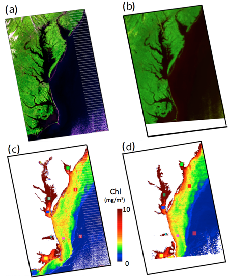
For the Suomi and Aqua satellite orbits, SNOs occur most frequently at high latitude polar regions [5]. Through analysis of orbital tracks of Suomi and Aqua, we identified a number of overlapping VIIRS and MODIS scenes over the Chesapeake Bay area. After screening out cloud-contaminated scenes, we were able to identify fairly clear pairs of VIIRS and MODIS images. Figure 1 shows MODIS and VIIRS images over the Chesapeake Bay area acquired on 10 January 2013. Figure 1a,b are MODIS and VIIRS images, respectively. The time difference between the two sensors passing over the Chesapeake Bay area was only about seven minutes. The solar zenith angles of the two sensors are both approximately 63 degrees. The view zenith angles at Chesapeake Bay areas are less than 20 degrees for both MODIS and VIIRS sensors.

Figure 1. Satellites image over the Chesapeake Bay, acquired on 10 January 2013: (a) Aqua-MODIS RGB image; (b) VIIRS RGB image; (c) MODIS chlorophyll concentration (mg/m³); and (d) VIIRS chlorophyll concentration (mg/m³). Eight regions of interest (ROIs) were randomly chosen for inter-sensor comparisons on the seven ocean color channels. The yellow star (*) in the image is the location where the HyperPro in situ measurement is made.

Figure 1. Satellites image over the Chesapeake Bay, acquired on 10 January 2013: (a) Aqua-MODIS RGB image; (b) VIIRS RGB image; (c) MODIS chlorophyll concentration (mg/m³); and (d) VIIRS chlorophyll concentration (mg/m³). Eight regions of interest (ROIs) were randomly chosen for inter-sensor comparisons on the seven ocean color channels. The yellow star (*) in the image is the location where the HyperPro in situ measurement is made.

Eight cloud-free water areas near the Chesapeake Bay, as marked in Figure 1, were randomly selected for inter-sensor comparison purposes. The radiances of the seven ocean color channels (see Table 1) and the corresponding retrieved ocean color products, such as normalized water-leaving radiances (nLw) and chlorophyll concentrations, are compared. In order to ensure the two sensors covered the same areas, we selected rectangular regions over homogeneous water areas with the same latitudes and longitudes at the four corners of each area. This reduced uncertainties associated with the spatial resolution of the two sensors. The yellow star (*) marked in the image is the location where the ground measurements from a HyperPro spectrometer were taken on the same day. The data acquisition times for MODIS-aqua, VIIRS, and the HyperPro spectrometer are 13:10, 13:03, and 11:10 EST, respectively. MODIS and VIIRS are multispectral sensors with 1000 m and 750 m spatial resolutions, while ground measurements from the HyperPro spectrometer are spatial point measurements and spectrally cover the contiguous wavelength range from 0.35 to 0.80 µm at a spectral resolution of 0.01 µm.

Vicarious calibration [12] is applied during atmospheric correction for ocean color applications. It is a process for establishing gain adjustments to improve and fine-tune sensor measurement. During atmospheric correction, nLw values are derived from the Lt values. To compute the vicariously calibrated gains, sensor scenes over in situ data locations are first processed with standard gains (gains equal to 1) for all spectral bands. During this process, atmospheric scattering and absorption factors, such as Rayleigh and aerosol scattering radiances and atmospheric gas absorption coefficients, are generated at each wavelength band. After the satellite-derived nLw values have been computed, the various scattering and absorption factors are still held in memory. To perform the vicarious calibration, the satellite-derived nLw values are then replaced by in situ nLw values. All the atmospheric correction scattering and absorption factors are then added to the in situ nLw values to estimate the Lt values that would yield these measured nLw values. Thus, these spectral vicarious total radiances (vLt) represent the adjusted Lt value needed to retrieve the in situ nLw measurements after atmospheric correction.

When vLt values are generated from multiple dates of imagery over in situ data locations, a multi-date statistical sample is established. The ratio of the vLt/Lt over this multi-day data set provides a vicariously calibrated gain factor for each wavelength that, when multiplied by the Lt value, provides a “tuned” Lt value that will yield more accurate nLw values after atmospheric correction. All pixels in the same scene (i.e., away from the in situ data locations), or scenes at other times can be processed using the vicariously calibrated gain factors.

NASA uses the Marine Optical Buoy (MOBY) [13], moored near Lanai, Hawaii, to provide in situ in-water measurements used in vicarious calibration of ocean color sensors. The resulting vicariously calibrated gains then become the accepted gains to use for the sensor. The MOBY and VIIRS vicariously calibrated gains used to process data in this study were generated using MOBY in situ data.

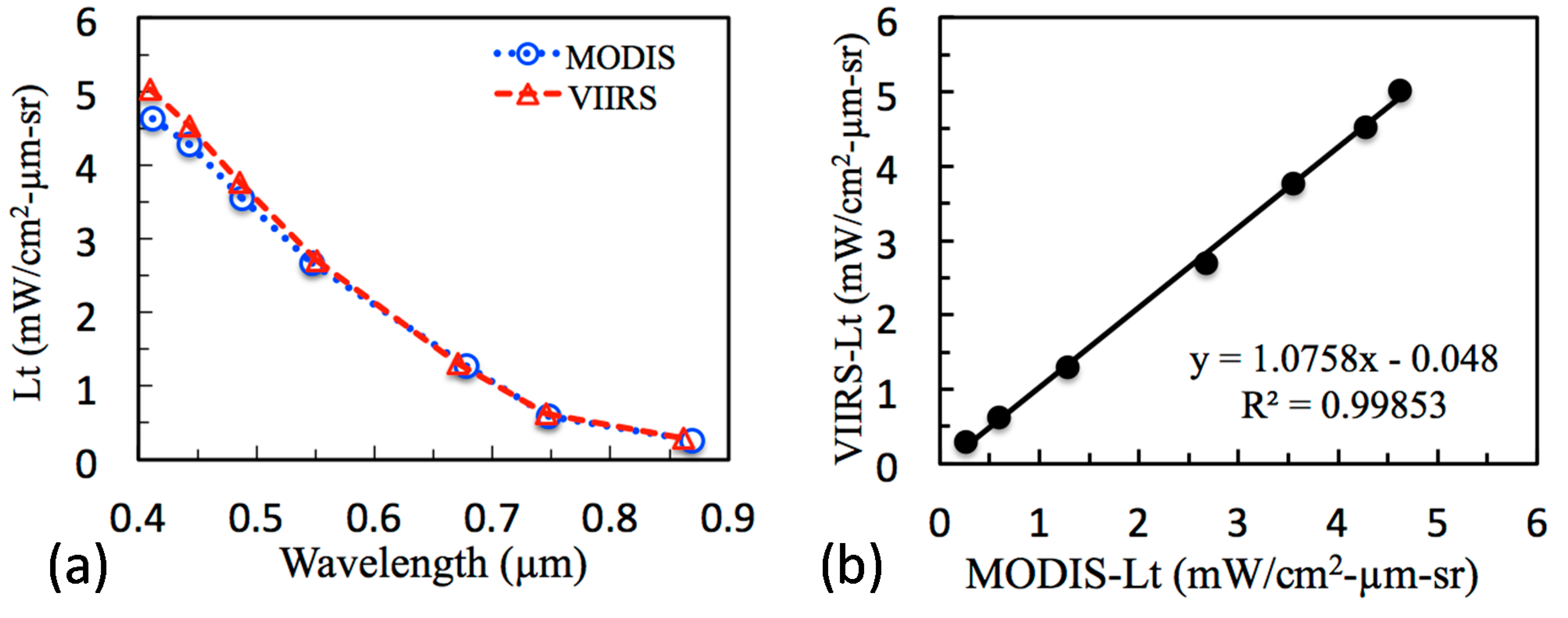
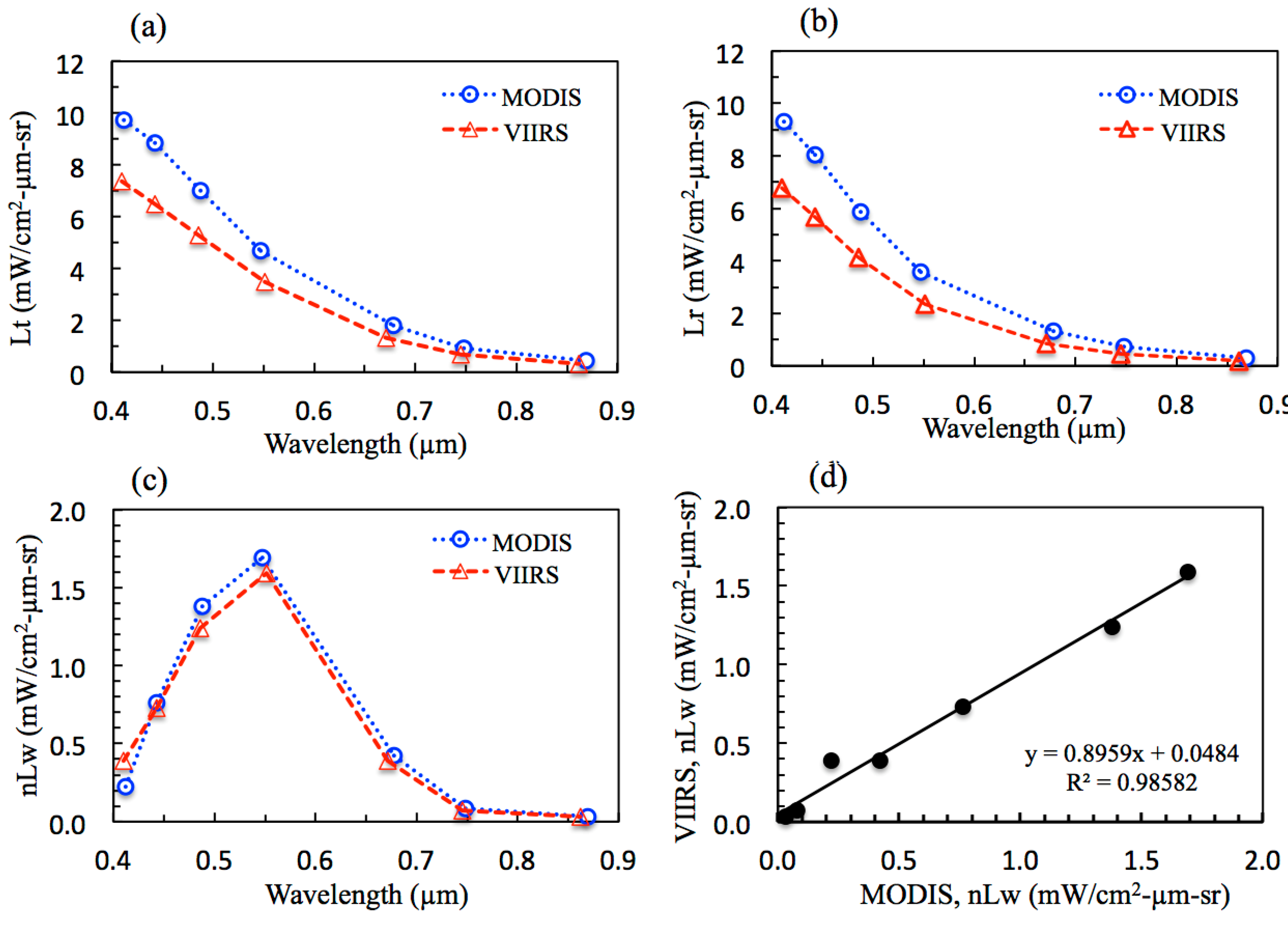
Figure 2a shows Lt measurements over Region 2. The dotted blue line is for the MODIS data, and the dashed red line for VIIRS data. The shapes of the spectral wavelength dependences, i.e., the decreases in radiances with increasing wavelengths, for both the MODIS and VIIRS data have similar spectral trends to the Rayleigh and aerosol scattering properties. The regression analysis of the scatter plot of the MODIS and VIIRS Lt measurements in Figure 2b has a high value of coefficient of determination (R²), where R is the correlation coefficient. The slope from the regression analysis is 1.08. The line in Figure 2b is a least-squares fit to the data, which contains the Lt measurements from seven channels of both sensors. If a data point in Figure 2b deviates from this line, we can conclude that there are differences in the radiometry for the corresponding MODIS or VIIRS channel. The use of the Figure 2b scatter plot to view data, in principle, allows for quick identification of possible band discrepancies between corresponding sensor bands. The 8% deviation from 1.0 in the slope could be attributed to sensor calibration, differences in derived Rayleigh scattering, and/or differences in derived aerosol scattering between the MODIS and VIIRS data.

Figure 2. (a) Top-of-Atmosphere multi-channel total radiances (Lt) in unit of mW/(cm²-µm-sr) of MODIS and VIIRS over Region 2, and (b) scatter plot of MODIS versus VIIRS Lt plus the best fit least-square regression line.

Figure 2. (a) Top-of-Atmosphere multi-channel total radiances (Lt) in unit of mW/(cm²-µm-sr) of MODIS and VIIRS over Region 2, and (b) scatter plot of MODIS versus VIIRS Lt plus the best fit least-square regression line.

The Automatic Processing System (APS) developed at NRL/SSC [14] was used to generate ocean color data products, such as water-leaving radiance and chlorophyll concentration, from both MODIS and VIIRS data. APS is based on, and is consistent with, the NASA SeaWiFS Data Analysis Software (SeaDAS). Figure 3a shows the nLw values retrieved from MODIS and VIIRS data over Region 2. After atmospheric corrections, the retrieved nLw curves of the two sensors coincide well. Figure 3b is the scatter plot of VIIRS versus MODIS normalized water-leaving radiances, which are shown in Figure 3a. A regression analysis of the seven channels in Figure 3b gives a slope of 0.96 with a very high R² value. This demonstrates good agreement between derived VIIRS and MODIS nLw across all wavelengths using APS atmospheric correction.

Figure 3. (a) Multi-channel normalized water-leaving radiances (nLw) of MODIS and VIIRS over Region 2 retrieved by APS, and (b) scatter plot of VIIRS versus MODIS nLw with the best-fit least-squares regression line.

Figure 3. (a) Multi-channel normalized water-leaving radiances (nLw) of MODIS and VIIRS over Region 2 retrieved by APS, and (b) scatter plot of VIIRS versus MODIS nLw with the best-fit least-squares regression line.

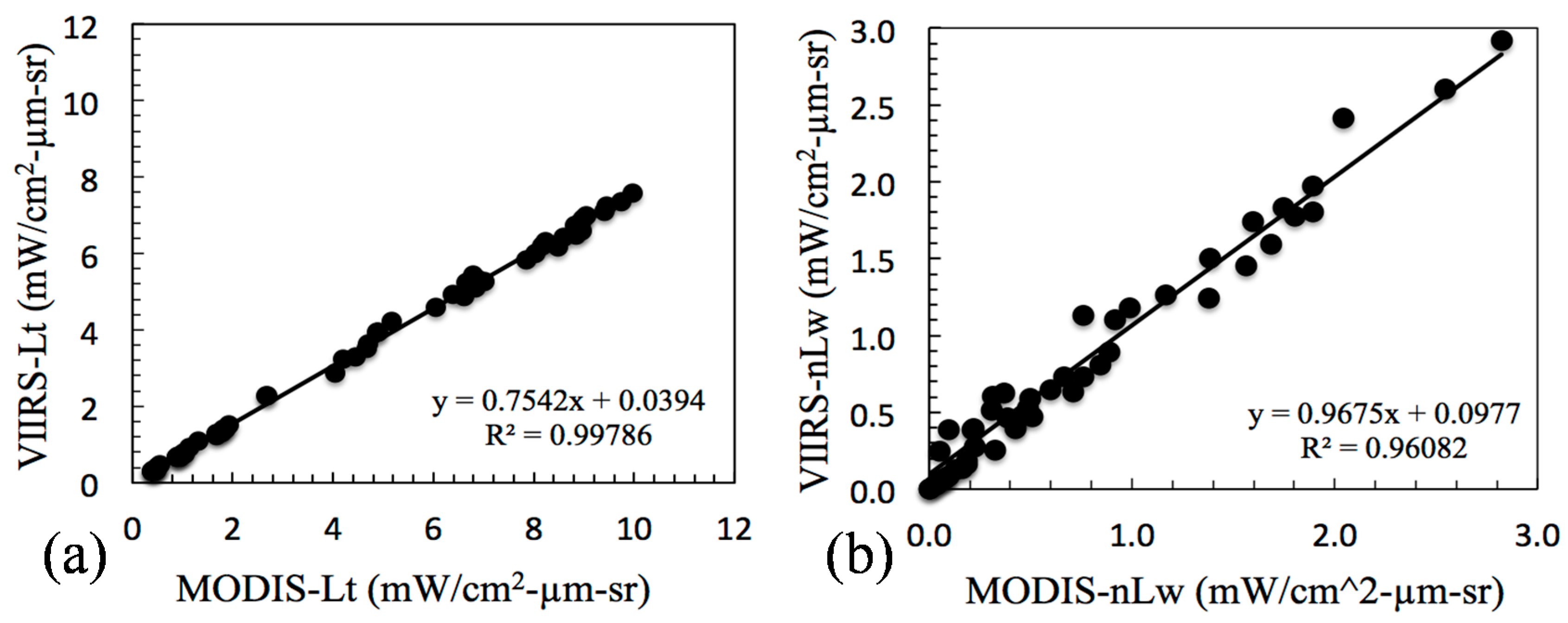
To further demonstrate the agreements between VIIRS and MODIS, in Figure 4a we show the scatter plot of VIIRS versus MODIS Lt measurements for seven ocean color channels at the eight selected surface areas, as marked in Figure 1. Regression analysis, shown in Figure 4a, has a slope of 1.07 and an offset of 0.05. This indicates that the VIIRS Lt is about 7% higher than that of MODIS, considering all wavelengths and at all 8 locations. Figure 4b shows the scatter plot of the MODIS and VIIRS APS-derived nLw estimates for all channels and at all 8 locations. The regression analysis in Figure 4b shows that all the data points are tightly clustered around a line with a slope of 0.94 and a small offset. The differences between APS-retrieved VIIRS and MODIS nLw estimates are approximately 10%, with VIIRS lower than MODIS. This is a good agreement in view of the fact that roughly 80%–90% of atmospheric scattered path radiances in Figure 4a are removed from the Lt measurement when computing the nLw during the atmospheric correction process.

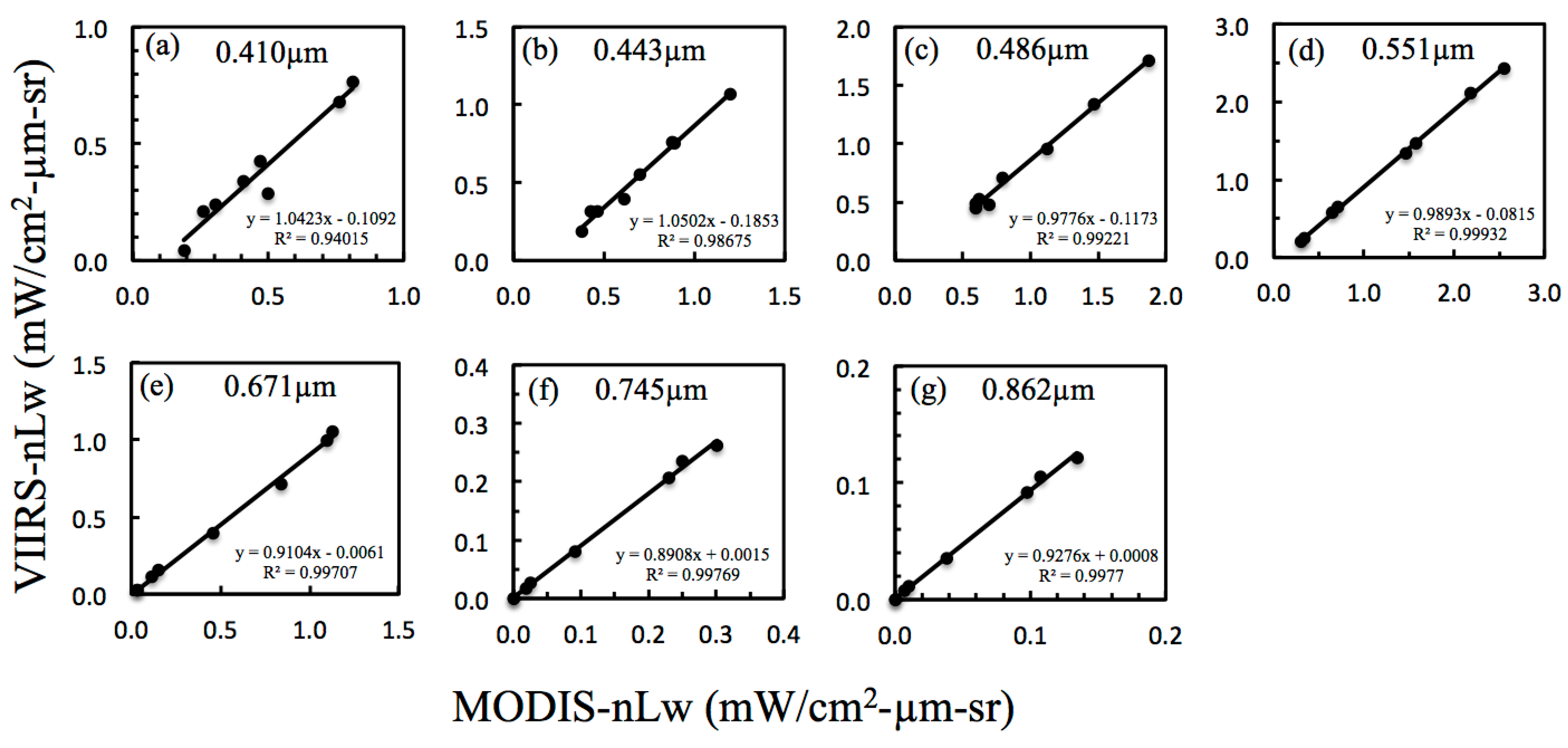
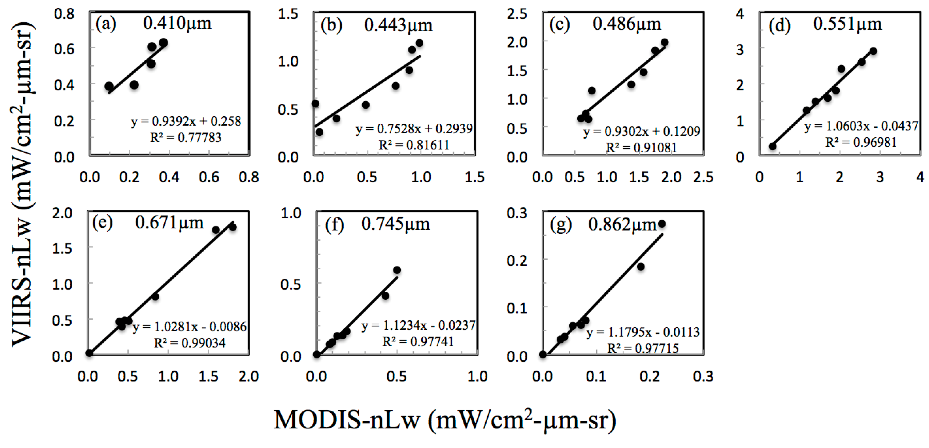
In order to evaluate the retrieval results on a channel-by-channel basis, we did the inter-comparison for each channel. Figure 5 shows the scatter plots of nLw for each wavelength over the eight locations, as marked in Figure 1. The least square fitting lines and R² values are calculated at each wavelength, and are shown in each plot on Figure 5. These R² values provide information on how well the data are matched between sensors for each channel. The results show that, for the channels at 0.443 µm or longer wavelengths, the VIIRS-nLw and MODIS-nLw agreed well with high R² values. For the 0.410-µm channel, the retrieved nLw values were not clustered as tightly as the other channels, but still had R² values greater than 0.9. The inconsistency can be attributed to minor errors in sensors’ calibrations and atmospheric corrections.

Figure 4. (a) Scatter plot of VIIRS versus MODIS Lt measurements for the eight locations marked in Figure 1, and (b) Scatter plot of VIIRS versus MODIS APS-derived nLw estimates for the eight locations with the best-fit least-squares regression line.

Figure 4. (a) Scatter plot of VIIRS versus MODIS Lt measurements for the eight locations marked in Figure 1, and (b) Scatter plot of VIIRS versus MODIS APS-derived nLw estimates for the eight locations with the best-fit least-squares regression line.

Figure 5. Scatter plots of VIIRS versus MODIS APS derived nLw estimates for the eight locations marked in Figure 1 and with each of the seven ocean color channels plotted separately.

Figure 5. Scatter plots of VIIRS versus MODIS APS derived nLw estimates for the eight locations marked in Figure 1 and with each of the seven ocean color channels plotted separately.

Table 2. Statistical results on the comparisons of nLw between MODIS and VIIRS for data collected over Chesapeake Bay areas on 10 January 2013.

Parameters	0.410 µm	0.443 µm	0.486 µm	0.551 µm	0.671 µm	0.745 µm	0.862 µm	Overall
N	8	8	8	8	8	8	8	56
Regression	1.042x − 0.109	1.05x − 0.185	0.978x − 0.117	0.989x − 0.082	0.910x − 0.006	0.891x + 0.002	0.928x + 0.001	0.97x − 0.071
R2	0.940	0.9867	0.9922	0.9993	0.9971	0.998	0.998	0.987
PD (%)	25.37	25.70	16.53	12.87	14.81	5.87	0.94	14.58
APD (%)	25.37	25.70	16.53	12.87	14.89	8.66	7.74	15.97

Table 2. Statistical results on the comparisons of nLw between MODIS and VIIRS for data collected over Chesapeake Bay areas on 10 January 2013.

Parameters	0.410 µm	0.443 µm	0.486 µm	0.551 µm	0.671 µm	0.745 µm	0.862 µm	Overall
N	8	8	8	8	8	8	8	56
Regression	1.042x − 0.109	1.05x − 0.185	0.978x − 0.117	0.989x − 0.082	0.910x − 0.006	0.891x + 0.002	0.928x + 0.001	0.97x − 0.071
R2	0.940	0.9867	0.9922	0.9993	0.9971	0.998	0.998	0.987
PD (%)	25.37	25.70	16.53	12.87	14.81	5.87	0.94	14.58
APD (%)	25.37	25.70	16.53	12.87	14.89	8.66	7.74	15.97

The fitting results for each wavelength and for data acquired on 10 January 2013 are summarized in Table 2. Here, the average Percent Differences is denoted as PD, and the average Absolute Percent Differences denoted as APD of N total number of locations. PD determines the bias between the quantities being compared, while APD estimates the average uncertainty [15]. The values of PD are calculated by averaging the percent differences between the matchups of the individual observations. Percentage difference of the jth matchup, PDj, is calculated by:

$$P{D}_j=100 *\frac{\left({{\displaystyle \sum }}_{i=0}^{N-1}\frac{\left(M_{j,i}-V_{j,i}\right)}{M_{j,i }}\right)}{N}$$

(1)

where i is the index for the samples, j for the sensor channels, N the total number of locations in the comparisons, and V_j,i and M_j,i stand for the VIIRS and MODIS data at the jth channel and the ith sample, respectively. Similarly, APD_j values are calculated by the following:

$$AP{D}_j=100*\frac{\left({{\displaystyle \sum }}_{i=0}^{N-1}\frac{\left|M_{j,i}-V_{j,i}\right|}{M_{j,i }}\right)}{N}$$

(2)

To verify the validity of the VIIRS and MODIS nLw estimates, we also compared them with in situ measured nLw data collected with the HyperPro hyperspectral radiometer in the Chesapeake Bay area, which is marked with a yellow star (*) in Figure 1 images. The HyperPro spectral measurements were made on the same day, approximately two hours prior to the VIIRS and MODIS overpasses. Figure 6 shows the nLw as a function of wavelength from VIIRS, Aqua MODIS, and HyperPro. The MODIS data are represented by the circles, VIIRS by the triangles, and HyperPro by the plus. Since MODIS and VIIRS are multi-channel sensors, they do not have the spectral resolution that HyperPro does. In general, the nLw values from the three sensors are comparable although those from the satellite data are lower than those from the ground measurements, especially in short wavelength regions. Multiple factors, such as the spatial resolution of the satellite sensors (MODIS spatial resolution is 1 km and VIIRS is 750 m) versus point measurements from the HyperPro and possible errors in atmospheric correction of the satellite data, are likely responsible for the discrepancies.

It should be pointed out that both VIIRS and MODIS lack narrow channels to capture the weak water-leaving radiance peak centered near 0.70 µm. The two instruments also lack narrow channels to capture the major water-leaving radiance peak centered near 0.58 µm. Therefore, both the multi-channel VIIRS and MODIS instruments are unable to capture the full spectral information contained in the HyperPro-measured normalized water-leaving radiance spectrum over a turbid water area.

Figure 6. A comparison of normalized water-leaving radiances (nLw) retrieved on 10 January 2013 from VIIRS data, MODIS data, and a field-measured spectrum over a turbid water area in the Chesapeake Bay.

Figure 6. A comparison of normalized water-leaving radiances (nLw) retrieved on 10 January 2013 from VIIRS data, MODIS data, and a field-measured spectrum over a turbid water area in the Chesapeake Bay.

The retrieved chlorophyll concentrations (chl) from APS for MODIS and VIIRS data are shown in Figure 1c,d. The chlorophyll variation patterns in both images are quite similar. Figure 7 shows the scatter plot of VIIRS chlorophyll concentration versus MODIS chlorophyll concentration for the selected regions marked in the Figure 1 images. A regression analysis of these data points produced a line with a slope of 1.09 and offset of 0.07 with R² value of 0.985.

Figure 7. Scatter plot of VIIRS chlorophyll concentration versus MODIS chlorophyll concentration from coincident scenes on 10 January 2013, for the selected regions marked in Figure 1 images with the best-fit least-squares regression line.

Figure 7. Scatter plot of VIIRS chlorophyll concentration versus MODIS chlorophyll concentration from coincident scenes on 10 January 2013, for the selected regions marked in Figure 1 images with the best-fit least-squares regression line.

3.2. Measurements with Large Differences in View Zenith Angles

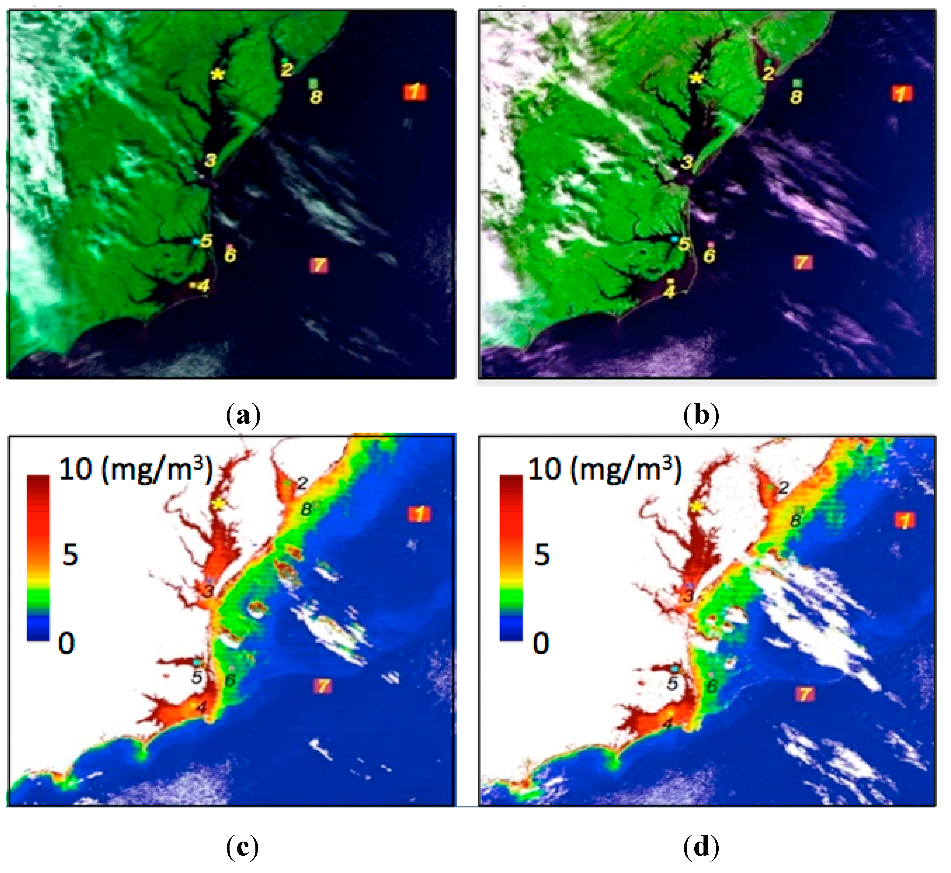
As described previously, due to the intrinsic Suomi VIIRS and Aqua MODIS satellite orbital properties, it is very difficult to find coincident cloud-free SNO VIIRS and MODIS scenes over the Chesapeake Bay area.  However, because of large swath widths of both sensors, coincident cloud-free scenes covering the Chesapeake Bay area with large differences in the sensor viewing angles can be found. Figure 8 shows a pair of VIIRS and MODIS images acquired on 9 March 2013. The Chesapeake Bay is located near nadir for VIIRS (Figure 8a), but close to the far right edge of the MODIS image (Figure 8b), as shown in yellow rectangular box. The sensor view angles over the Chesapeake Bay are approximately 25 degrees for VIIRS and 53 degrees for MODIS.

Figure 8. (a) VIIRS image and (b) MODIS image acquired over the Chesapeake Bay on 9 March 2013.

Figure 8. (a) VIIRS image and (b) MODIS image acquired over the Chesapeake Bay on 9 March 2013.

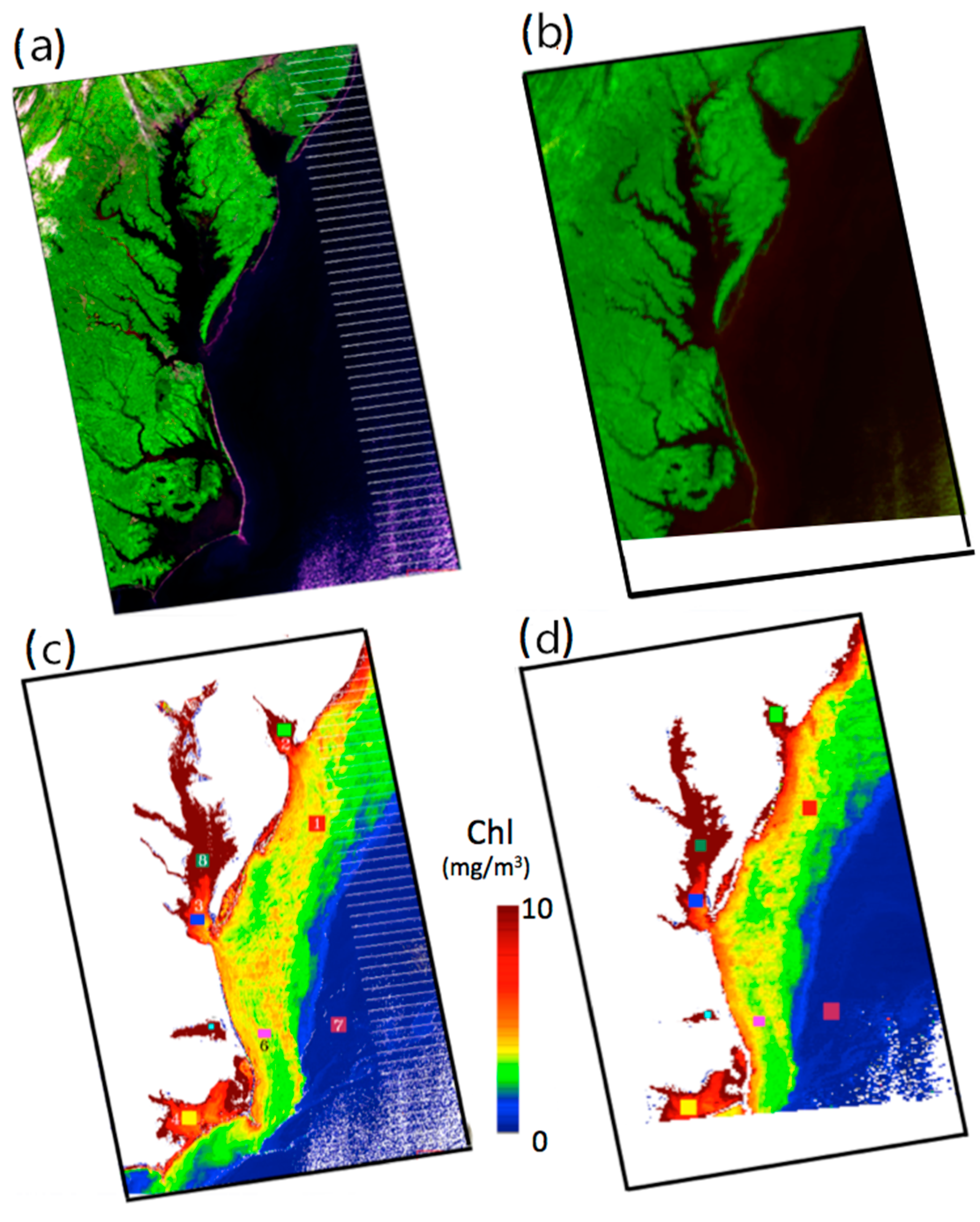
Figure 9a shows portions of the VIIRS image (after geo-registration) covering the Chesapeake Bay area. The parallel white lines in this image do not contain real VIIRS data but represent data gaps due to the VIIRS read out circuit design for data at higher sensor zenith angles. Figure 9b is for the corresponding MODIS image. Figure 9c is the APS-derived chlorophyll concentration image from the VIIRS data, while Figure 9d is the chlorophyll concentration image obtained from MODIS data.

For inter-sensor comparisons, eight areas similar to the locations shown in Figure 1 are marked in Figure 9c,d. Figure 10a shows the Lt measurements over Region 1. The dotted line is for the multi-channel MODIS data, and the dashed line for the VIIRS data. Due to view angle differences between MODIS and VIIRS, the MODIS scene had significantly more Rayleigh scattered radiance (Lr) than the VIIRS scene. This is confirmed in Figure 10b, in which the APS-calculated Lr for MODIS and VIIRS based on solar and view angles are shown. Figure 10c shows the nLw estimates retrieved from MODIS and VIIRS data over the region. Although the Lt radiances of MODIS and VIIRS (Figure 10a) are quite different, the retrieved nLw are well matched (Figure 10c). This is due, in part, to the fact that a larger Lr value was subtracted out from the MODIS Lt in the atmospheric correction process. Figure 10d is the scatter plot of VIIRS versus MODIS nLw values, as shown in Figure 10c. A regression analysis of the seven channel data points in Figure 10d gives a slope of 0.896 and offset 0.0484 with a high R² value. The plots in Figure 10, in particular Figure 10c, have demonstrated that nLw can be recovered reasonably well regardless of the sensor view angles.

Figure 9. Satellite images over the Chesapeake Bay acquired on 9 March 2013: (a) VIIRS RGB image; (b) MODIS RGB image; (c) VIIRS Chlorophyll concentration; and (d) MODIS Chlorophyll concentration.

Figure 9. Satellite images over the Chesapeake Bay acquired on 9 March 2013: (a) VIIRS RGB image; (b) MODIS RGB image; (c) VIIRS Chlorophyll concentration; and (d) MODIS Chlorophyll concentration.

Figure 10. (a) Top-of-Atmosphere multi-channel radiances (Lt) of MODIS and VIIRS over Region 1; (b) APS-calculated Rayleigh path radiances (Lr) of MODIS and VIIRS; (c) Spectra of normalized water-leaving radiances (nLw) of MODIS and VIIRS retrieved with APS; and (d) scatter plot of VIIRS versus MODIS nLw estimates.

Figure 10. (a) Top-of-Atmosphere multi-channel radiances (Lt) of MODIS and VIIRS over Region 1; (b) APS-calculated Rayleigh path radiances (Lr) of MODIS and VIIRS; (c) Spectra of normalized water-leaving radiances (nLw) of MODIS and VIIRS retrieved with APS; and (d) scatter plot of VIIRS versus MODIS nLw estimates.

Figure 11. Data from MODIS and VIIRS imagery collected on 9 March 2013: (a) scatter plot of VIIRS versus MODIS Lt for the eight locations marked in Figure 9 with best-fit least-squares regression line, and (b) scatter plot of VIIRS versus MODIS nLw with best fit least-squares regression line.

Figure 11. Data from MODIS and VIIRS imagery collected on 9 March 2013: (a) scatter plot of VIIRS versus MODIS Lt for the eight locations marked in Figure 9 with best-fit least-squares regression line, and (b) scatter plot of VIIRS versus MODIS nLw with best fit least-squares regression line.

To increase the number of VIIRS and MODIS data for ocean color comparisons, we show in Figure 11a the scatter plot of VIIRS versus MODIS Lt for all eight selected regions, as marked in Figure 9 images, and with all seven channels listed in Table 1. A regression analysis using all the data points in Figure 11a gives a slope of about 0.754. MODIS-measured Lt values are about 25% higher than those of VIIRS. This is due to the larger view angles of the MODIS measurements (at the rightmost edge of Figure 8b) with longer path radiances and stronger Rayleigh scattering. Figure 11b is a scatter plot similar to Figure 11a but for the APS-derived nLw from the Figure 11a VIIRS and MODIS Lt. A regression analysis shows that all the data points in Figure 11b are clustered around a line with a slope of approximately 0.97 and a R² value of 0.96.

The detailed comparisons for each channel over the eight locations are shown in Figure 12. Each scatter plot represents nLw over all the locations, as marked in Figure 9. Regression analysis results are presented in each of the plots. For channels at 0.488 micron or longer wavelengths, the VIIRS-nLw and MODIS-nLw agreed well with high R² values. This demonstrates that nLw can be retrieved reasonably well from MODIS and VIIRS radiances acquired with large differences in satellite sensors’ view zenith angles, particularly for channels centered at 0.488 micron or longer wavelengths.

Figure 12. Scatter plots of VIIRS versus MODIS APS derived nLw estimates from 9 March 2013 for the eight locations marked in Figure 9 and with each of the seven ocean color channels plotted separately.

Figure 12. Scatter plots of VIIRS versus MODIS APS derived nLw estimates from 9 March 2013 for the eight locations marked in Figure 9 and with each of the seven ocean color channels plotted separately.

Table 3. Statistical results on the comparisons on nLw between MODIS and VIIRS for data collected over Chesapeake Bay areas on 9 March 2013.

Parameters	0.410 µm	0.443 µm	0.486 µm	0.551 µm	0.671 µm	0.745 µm	0.862 µm	Overall
N	5	8	8	8	8	8	8	53
Regression	0.939x + 0.258	0.753x + 0.294	0.930x + 0.121	1.060x − 0.044	1.028x − 0.0086	1.123x − 0.024	1.1795x − 0.0113	1.002x + 0.0836
R2	0.778	0.816	0.911	0.97	0.99	0.977	0.977	0.917
PD (%)	−43.06	−20.80	−5.89	−0.98	0.22	4.91	1.09	−9.215
APD (%)	34.45	16.65	12.99	9.30	8.36	10.59	9.79	14.589

Table 3. Statistical results on the comparisons on nLw between MODIS and VIIRS for data collected over Chesapeake Bay areas on 9 March 2013.

Parameters	0.410 µm	0.443 µm	0.486 µm	0.551 µm	0.671 µm	0.745 µm	0.862 µm	Overall
N	5	8	8	8	8	8	8	53
Regression	0.939x + 0.258	0.753x + 0.294	0.930x + 0.121	1.060x − 0.044	1.028x − 0.0086	1.123x − 0.024	1.1795x − 0.0113	1.002x + 0.0836
R2	0.778	0.816	0.911	0.97	0.99	0.977	0.977	0.917
PD (%)	−43.06	−20.80	−5.89	−0.98	0.22	4.91	1.09	−9.215
APD (%)	34.45	16.65	12.99	9.30	8.36	10.59	9.79	14.589

The regression analysis results on the comparisons for each wavelength for data acquired on 9 March 2013 are listed in Table 3. There are lower R² values for retrieved nLw estimates for the channels at 0.410 µm and 0.443 µm between MODIS and VIIRS, which can be attributed to errors in atmospheric correction procedures. For channels at 0.486 µm or longer wavelengths, there are higher R² values and smaller nLw differences.

4. Conclusions

We report on inter-sensor comparisons between VIIRS and MODIS data acquired over the Chesapeake Bay and nearby areas not only with SNO measurements, but also with relatively large differences in sensors’ zenith angles. We compare radiances at the top of the atmosphere and normalized water-leaving radiances and ocean color data products derived with the Automatic Processing System from both VIIRS and MODIS data. We observed that, although there are large differences between the measured radiances at the top of the atmosphere of the two sensors when there are significant differences in the sensor zenith angles, the retrieved ocean color products, such as normalized water-leaving radiances, matched approximately 15% (mean difference, averaged across all wavelengths). The results show that the variation in satellite view zenith angles is not a main factor affecting the retrieval of ocean color from different satellite sensors (i.e., the atmospheric correction routine adequately removes the view-angle dependence). Thus, VIIRS and MODIS provide consistent ocean color data that can generally be reliably merged to create fused composite imagery, even when viewing angles differ considerably.