A Robust Photogrammetric Processing Method of Low-Altitude UAV Images

Abstract

Low-altitude Unmanned Aerial Vehicles (UAV) images which include distortion, illumination variance, and large rotation angles are facing multiple challenges of image orientation and image processing. In this paper, a robust and convenient photogrammetric approach is proposed for processing low-altitude UAV images, involving a strip management method to automatically build a standardized regional aerial triangle (AT) network, a parallel inner orientation algorithm, a ground control points (GCPs) predicting method, and an improved Scale Invariant Feature Transform (SIFT) method to produce large number of evenly distributed reliable tie points for bundle adjustment (BA). A multi-view matching approach is improved to produce Digital Surface Models (DSM) and Digital Orthophoto Maps (DOM) for 3D visualization. Experimental results show that the proposed approach is robust and feasible for photogrammetric processing of low-altitude UAV images and 3D visualization of products.

1. Introduction

Low-altitude high-resolution images have great potential in many applications such as large scale mapping, true orthophoto generation, archaeology, 3D city modeling, and especially emergency response [1,2]. Low-altitude UAV has several advantages: flexibility, low cost, simplicity of operation, and ease of maintenance. Moreover, low-altitude UAV images provide a good alternative to satellite remote sensing and traditional aerial photogrammetry for high-resolution imagery. The typical large rotation angles of UAV images leads to no strictly predefined relationship between adjacent images, which is beyond the capability of traditional photogrammetric software [1,2]. Light low-altitude UAV usually embeds common single-lens reflex (SLR) digital cameras as sensors while lens distortions are simultaneously imported.

The key to success of applying the remote sensing images acquired by low-altitude UAV is aerial triangulation (AT). Light small-sized UAVs are not reliable enough so that the actual flight path cannot be always as straight as that of traditional aerial photogrammetry (strip deformation ≤3% demanded by China National Standard: GB/T 6962-2005). As a result, there are usually large overlap variations and large rotation angles between adjacent images [2]. Moreover, the image frame is so small that there are many more images than in traditional photogrammetry. These factors pose the following challenges for automatic AT: (1) The identification of ground control points (GCPs) is time-consuming because of the large number of images and the irregular overlap; (2) Because of the large rotation angles, differences in scale and overlap are apparent, and the success rate of image correlation is decreased, which has a strong impact on automatic extraction and distribution of tie points, even possibly leading to the failure of AT.

2. Related Research

Automated AT in traditional aerial photogrammetry is relatively mature, and a large number of commercial software packages are available in the market, for instance, Z/I Imaging’s MATCH-AT and VirtuoZo [3]. However, these software packages with standard AT procedures are imperfectly suited for orientation of images with irregular overlap acquired by UAVs. In recent years, some procedures for the automated extraction of a consistent and redundant sets of tie points from markerless close-range or UAV images have been developed for photogrammetric applications [2,4,5]. Some commercial packages have also appeared on the market (e.g., PhotoModeler Scanner, Eos Inc; PostFlight Suite, Pix4D). Some free web-based approaches (e.g., Photosynth, 123DCatch, etc.) and open-source solutions (VisualSFM [6], Apero [7] and Bundler [8], etc.) are also available, although generally not reliable and accurate enough in case of large and complex image blocks with variable baselines and image scale [9]. The accuracy of Global Positioning System/Inertial Navigation System (GPS/INS), usually referred to as the Position and Orientation System (POS), on the light UAV cannot be used for direct geo-referencing to satisfy the high metric quality in the surveying applications. Thus, the orientation phase can rely on an image-based approach [2].

The geometry of the topological relations between UAV images is complex; therefore, it is difficult for traditional aerial photogrammetry software (such as VirtuoZo v3.6) to generate stable tie points. To reduce the time required for image-pair matching and to decrease the number of wrong matching relationships, a variety of ideas have been proposed by different researchers. Barazzetti et al. matched ordered images with every three images composing a set and obtained tie points which are visible in more than three images, but linear accumulated error exists in this method [10]. Two ideas are proposed in another paper by Barazzetti: to obtain a visibility map between images by fast processing of thumbnail images, and to estimate image overlap using GPS/INS and Digital Terrain Model (DTM) or Digital Surface Model (DSM) [11]. Haala [12] used a method similar to the idea of obtaining a visibility map that the connection relations were obtained by processing a set of images using the open-source Bundler [8] software. The method used in this paper is similar to the second idea of estimating image overlap with GPS/INS and DTM data to generate the connection map.

As for the computer vision research tasks without no accuracy requirements, distortion correction of images is not an essential step. As is known to all, the widely used “Structure from Motion (SfM)” approach put much focus on the automatic process of a large number of images, typically the match, orientation and 3D reconstruction [13,14,15,16,17]. When using photogrammetry to obtain accurate geographical information, measurable images without distortion are essential, and orientation matters for GCPs. In commercial aerial photogrammetry software, GCPs are generally recognized manually. Some software (such as LPS, Inpho, and VirtuoZo) calculates exterior orientation elements (EO) using more than three GCPs according to the collinearity equation and then calculates their positions in images by projection. There are not enough GCPs in one UAV image whose frame is small, while one control point may appear in several images. Hence, a proposed method of predicting GCPs in an image frame in this paper could improve the identification step.

In most situations, the automatic AT for low-altitude UAV images is similar to that for close-range images. The Scale Invariant Feature Transform (SIFT) [18,19] is widely adopted to obtain scale-invariant feature points and coarse matching points in close-range images and UAV images [1,2,10]. Then, the RANdom SAmple Consensus (RANSAC) [20] algorithm with the epipolar constraint or relative orientation method can be used to remove erroneous match points. With these correct match points as initial values, other feature extraction methods like those proposed by Förstner [21] and Harris [22] can be used to obtain precise match points. Furthermore, the match points can be optimized by the least-squares matching method. Finally, EOs of the UAV images are calculated using an adjustment. This is a typical method that was presented by Zhang [1]. Other similar methods include PreSync [4,23] which uses directly the points matched by the Kolor Autopono software and then obtains the EO by combining initial exterior orientation parameters and reference images after several iterations; ATiPE [10,17], which extracts “Features from Accelerated Segment Test” (FAST) [24] interest points after using the SIFT features to carry out least-squares matching of multiple images to obtain more tie points and to improve AT accuracy.

These approaches aforementioned try to improve the AT by raising the accuracy and redundancy of the tie point. Towards the same target, an improved SIFT feature extraction method and matching strategy for AT processing of UAV images is proposed in this paper. In this method, evenly distributed tie points are obtained automatically and output to the commercial block adjustment program PATB [25] for adjustment, thus eliminating the feature-point (including corner-point) extraction and matching operation following the SIFT matching step in other methods and improving efficiency. In addition, to create regional geometric networks to meet the requirements of aerial photogrammetric processing for images acquired by low-altitude weakly controlled UAV, a strip management method using UAV flight-control data to calculate connections between image pairs is proposed. To deal with distortion rectification and inner orientation of small-format non-metric UAV images of a size 10 times smaller than traditional aerial images, a parallel inner orientation-processing algorithm based on lookup tables is presented in this paper. A GCP estimation method using SIFT matching results is proposed to reduce the large workload of GCP identification in UAV images. Experiments confirm that the methods proposed in this paper are simple, convenient, and easy to implement.

The structure of this article is as follows: the proposed methodology for AT of UAV images, the low-altitude UAV system, and the experimental datasets are introduced in the following section. Next, the workflow is introduced in detail in Section 4, including the strip management method, the inner orientation method, the improved SIFT matching algorithm, the bundle adjustment (BA) calculation, and the generation and 3D visualization of Digital Elevation Model (DEM) and Digital Orthophoto Maps (DOM). Section 5 describes the experimental results of AT and the product. Conclusions and topics for further research are given in Section 6.

3. General Strategy and Data Acquisition

3.1. Strategy

When UAV is used in disaster emergencies and other emergency-response situations, it is absolutely necessary for the images to be processed immediately, and therefore a stable, easy, and efficient orientation method is of vital importance in AT. The first step in this paper is to estimate the overlapping connections of adjacent images using flight-control data. Second, a parallel algorithm based on mapping lookup tables accelerates the speed of inner orientation. An improved SIFT extracting and matching algorithm can obtain tie points from a large number of image pairs. The matching result is also used to estimate the image locations of GCPs in the GCP identification. After the matched tie points and GCPs have been transferred to the PATB software [25] for BA, the EOs of the images can be obtained. DEM and DOM can be generated with a high-density point cloud obtained by the dense point matching algorithm. According to the World Wind data organization model, 3D visualization can be implemented by overlaying of DEM and DOM. Figure 1 shows the research workflow of this paper, and the numbering indicates the section where the procedure is described.

Figure 1. Workflow proposed in this paper.

Figure 1. Workflow proposed in this paper.

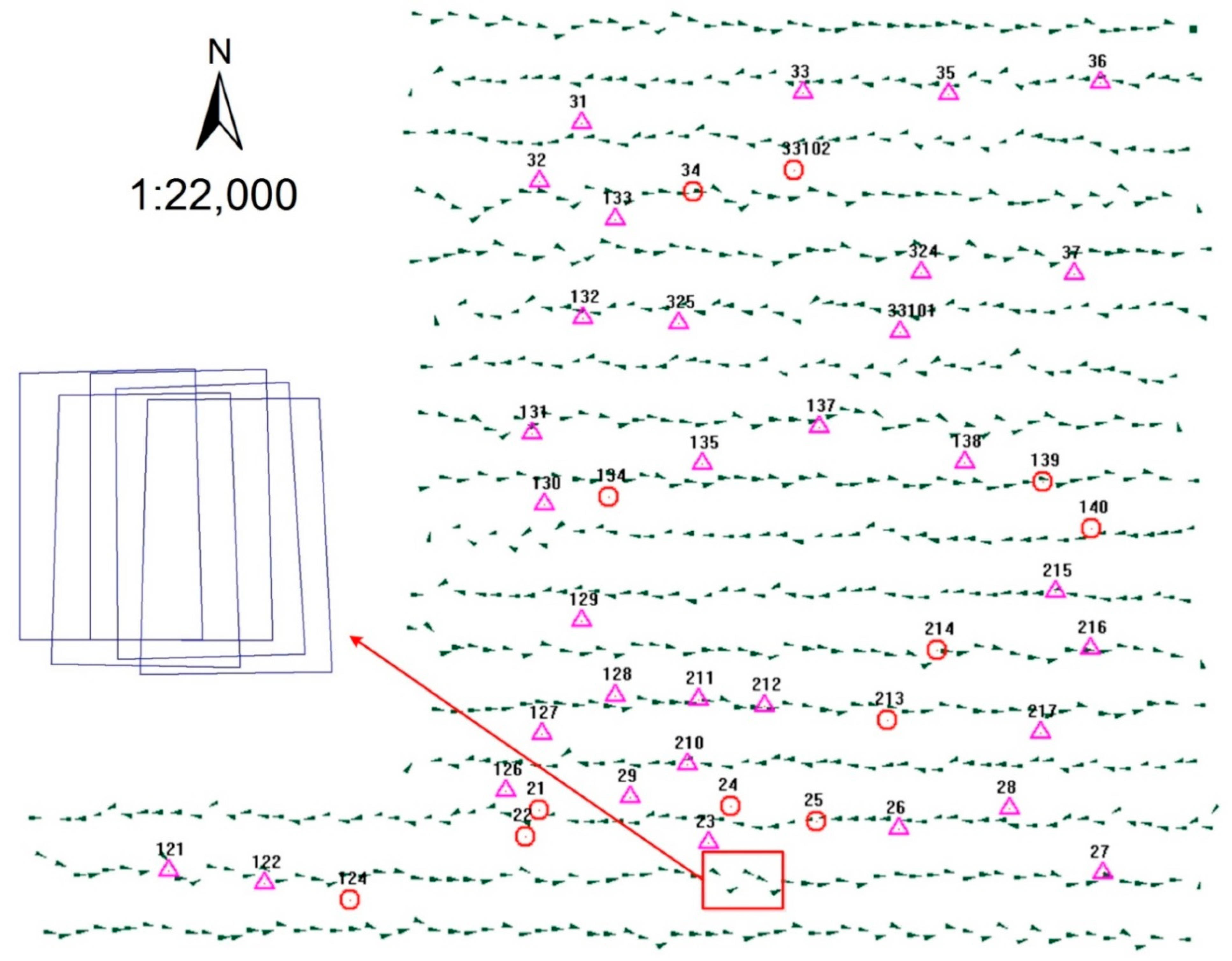
3.2. Experimental Dataset 1: Yangqiaodian

The UAV remote sensing platform used in the experiments of dataset 1 is composed of a fixed-wing aircraft, an image sensor, a programmable flight-management system with micro-POS for navigation and ground monitoring system. The UAV can fly along the scheduled trajectory taking images at locations scheduled by the programmable flight-management system that can provide the approximate position and attitude of the UAV at each exposure. As the POS is usually not precise enough as the light fixed-wing UAV is easy to be influenced by the wind, the footprints of UAV images are not the same as scheduled. The length of the vehicle is approximately 2 m, the wingspan is 2.5 m, the payload is 4 kg, and the flight speed is about 100 km/h. The remote imaging sensor on the UAV is a Canon 450D SLR camera with a fixed focal length of 24.314 mm which has been calibrated by the UAV provider. The image format is 2848 × 4272 pixels (each pixel is approximately 5.2 μm on the sensor), and the ground resolution is approximately 10 cm when the flight altitudes range from 575 to 605 m.

After confirming the acquisition requirement for aerial photogrammetry data, we should make the flight plan according to the tasks to be performed and the actual terrain before the UAV flights are carried out on in field. For these experiments, images were acquired by the UAV in a hilly area named Yangqiaodian in central China.

In May 2010, 854 images were acquired by the UAV system covering a hilly area in central China where the ground elevation varies from 25 to 60 m. These images belong to 17 flight strips in east-west direction. The longest flight route is approximately 4.8 km, the shortest flight route is approximately 3.4 km, the flight span is about 3.4 km, and the area is approximately 12.88 square kilometers. As shown in Figure 2, small sharp triangles represent the image center, and the orientation of the triangles represents the flight direction. There are 45 GCPs in the experiment, and the numbers represent the identifiers of GCPs. The 33 points indicated by equilateral triangles are used as control points, while the remaining 12 points marked by circles are check points for the bundle adjustment experiments. Figure 2 shows these flight strips are not in straight lines, they compose curved lines. The flight-control data indicates that (1) the average image rotation angle in this area is 9.93°, the largest image rotation angle is 49.22°; (2) the average flight-path deviation, defined as the distance from the center of footprint to the line composed of two neighbor centers in the same flight strip, is 16.61 m, while the largest distance is 74 m; (3) the overlap of images is somewhat irregular because the maximum forward overlap is 93%, while the minimum is 67%; (4) the maximum side overlap is 75% and the minimum is 40%. Figure 3 illustrates five typical images outlined in Figure 2.

Figure 4 shows the layout of the control points. On the ground, a white circle area approximately 1 m in diameter is brushed with lime and the coordinates of the center is surveyed by the GPS Real Time Kinematic (RTK) method before the flight. The precision of the GCPs is 0.02 m, and they are identified by their centers during the post-processing.

3.3. Experimental Dataset 2: PDS

This image dataset was acquired by another fixed-wing aircraft. The remote imaging sensor is a camera of SWDC-5 [26] with a fixed focal length of 82 mm which has been calibrated by the provider. The image format is 5362 × 7244 pixels (each pixel is approximately 6.8 μm on the sensor), and the ground resolution is approximately 5 cm when the flight altitudes range from 585 to 615 m.

Figure 2. Schematic drawing of Yangqiaodian.

Figure 2. Schematic drawing of Yangqiaodian.

Figure 3. Typical images of Yangqiaodian.

Figure 3. Typical images of Yangqiaodian.

In May 2011, 165 images were acquired which were covering an urban area named PDS in central China where the ground elevation varies from 80–130 m. These images belong to seven flight strips in east-west direction. Eighty images are chosen for our experiment, namely the images in red rectangle in the following Figure 5. The average of flight route is approximately 2.3 km; the flight span is about 1.5 km. There are 85 GCPs in the experimental area and their planimetric and height accuracy are approximate 0.01 m. The 14 out of 85 points indicated by red circles are used as check points for the bundle adjustment experiments. Figure 5 shows the overlap of images is somewhat irregular because of the wind during the flight. The average of forward overlap is 63% and the maximum forward overlap is 75%, while the minimum is 31%. The average of side overlap is 40% and the maximum side overlap is 50% and the minimum is 31%. Figure 6 displays several typical images of PDS dataset.

Figure 4. Layout of control points in Yangqiaodian and image positions of Ground Control Points.

Figure 4. Layout of control points in Yangqiaodian and image positions of Ground Control Points.

Based on the layout principle of GCP in photogrammetry [27], there should be one GCP every three baselines along the flight direction and two GCPs every two baselines perpendicular to the flight direction. However, the numbers of total GCPs located in our study areas are different from the expected ones according to the aforementioned standard. This is primarily due to the actual landscape in our study areas which is highly different from the ideal situation. The recognizable obstacles including rivers, lakes, buildings, and hills make it difficult to have the distribution of GCP as the expected design with the exact calculated number. Similar situation exists in the experiments of Zhang’s paper [1]. Since such limitation cannot be avoided, we set our GCPs in the study areas according to the standard as likely as possible. Although there are slightly less GCPs in the study area of Yangqiaodian but more GCPs in the area of PDS, the overall accuracy is still acceptable and does not show significant influence on the experiments.

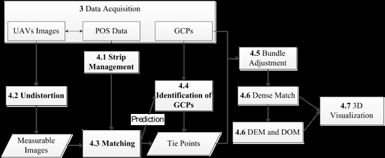
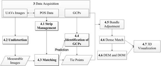
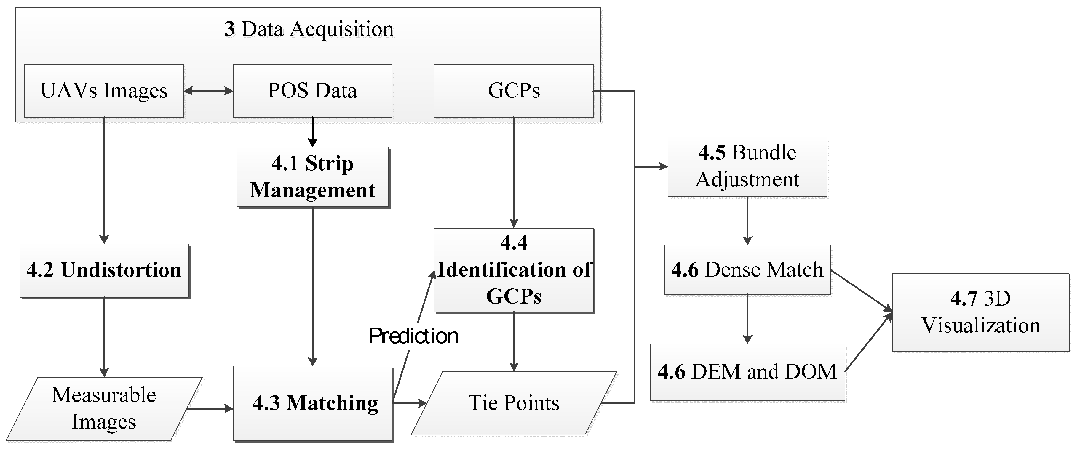
4. Photogrammetric Processing of UAV Images

4.1. Strip Management

The weak control of our UAV platform results in irregular forward and sideways overlap, and the complex connections between the images influences matching efficiency and AT accuracy. In this research, the topological connection map of the UAV images is generated using position and attitude data obtained by the weak control system including GPS/INS unit on the low-altitude UAV platform.

The images taken when the UAV is landing or turning around can be deleted according to the yaw angle (κ), and the result of this automated operation has been shown in Figure 2 and Figure 6.

The deflection angle β of an image’s center point decides whether the image belongs to a flight strip as β must be less than a given threshold determined in accordance with the low-altitude UAV digital aerial technical specifications.

Figure 5. The footprints of images in the experimental area of PDS.

Figure 5. The footprints of images in the experimental area of PDS.

Figure 6. Typical images of PDS dataset.

Figure 6. Typical images of PDS dataset.

The UAV flight control data records the camera position (Xs, Ys, Zs), pitch angle φ, roll angle ω, and yaw angle κ at each shooting moment, which can be regarded as rough EOs of each image. Then, the field of view (FOV) of each image is calculated in geodetic coordinates via the collinear equation, as shown in Equation (1):

$$\begin{gathered} X=X_S+(Z-Z_S)\frac{a_{1}x+a_{2}y-a_{3}f}{c_{1}x+c_{2}y-c_{3}f} \\ Y=Y_S+(Z-Z_S)\frac{b_{1}x+b_{2}y-b_{3}f}{c_{1}x+c_{2}y-c_{3}f} \end{gathered}$$

(1)

where f is the focal length (mm); Z is the average elevation of the area, which can be entered by the user or replaced by the average elevation of all the GCPs; Xs, Ys, Zs is the camera projection center under geodetic coordinates; a_i, b_i, c_i (i = 1, 2, 3) are nine elements from the rotation matrix calculated from each image’s φ, ω, and κ; (x,y) are the image coordinates of the pixels (mm); and (X,Y) are the corresponding geodetic coordinates. According to Equation (1), FOV of each image can be determined, and then the overlap between the images in the same strip and across strips can be calculated.

In this paper, the visualization of the connection map is partly displayed in Figure 7. A connection line between two images indicates that there is overlap between them. If there is no line between any pair of images, matching operation of this pair is skipped, which can effectively reduce the number of match operations and the matching error.

Figure 7. Connections of image pairs.

Figure 7. Connections of image pairs.

4.2. Geometric Correction

In this research, the coordinate transformation of corresponding image points before and after correction can be fitted with an appropriate polynomial as in Equation (2):

$$\begin{gathered} \Delta x=(x-x_0)(k_1{r}^2+k_2{r}^4)+p_1[r^2+2{(x-x_0)}^2]+2p_2(x-x_0)(y-y_0)+\text{α}(x-x_0)+\text{β}(y-y_0) \\ \Delta y=(y-y_0)(k_1{r}^2+k_2{r}^4)+p_2[r^2+2{(y-y_0)}^2]+2p_1(x-x_0)(y-y_0) \end{gathered}$$

(2)

where ∆x,∆y are the correction values of an image point; x,y are the coordinates in the image coordinate system, x0,y0 is the principal point, and $r=\sqrt{{(x-x_0)}^2+{(y-y_0)}^2}$, k₁ and k₂ are radial distortion coefficient, while P₁ and P₂ are tangential distortion coefficient, α and β are two scalars in the two image axes. In this paper, (∆x, ∆y)_[i][j] is the correction value for the image pixel (i, j).

For a non-metric camera, when the focal length is fixed, the lens distortion is a component of system error; it has the same effect on each UAV image. The lookup table-based distortion correction algorithm proposed in this paper corrects one image at a time with the same distortion parameters. The first UAV image is corrected by using the proposed distortion model, and all the correction value (∆x, ∆y)_[i][j] for all the image pixels are calculated and stored in a two-dimensional lookup table Array_[W][H], whose size is the same as the image. Then, the rest of the UAV images are corrected using the two-dimensional lookup table without calculating the correction values pixel by pixel. This lookup table accelerates image-distortion correction and avoids a mass of duplicate calculations.

To enhance efficiency, the OpenMP (Open Multi-Processing) [28] parallel processing technology is introduced in the accelerated distortion-correction algorithm. In OpenMP, many CPUs can work together to correct distortion, and one CPU deals with one image at a time.

A computer with a dual-core 2.80 GHz CPU and 2.00 GB memory is used to perform the experiment. Thirty images from the Yangqiaodian area are chosen for distortion removal with a direct distortion correction without any improvement, the lookup table-based distortion correction algorithm, and the parallel lookup table-based interior orientation method proposed in this paper. Table 1 shows the time required by these three methods.

Table 1. Time required by the three methods.

Method	First Image (s)	Remaining Images (s)	All (s)
Direct distortion correction	10.4	10.4	314.0
Lookup table-based distortion correction algorithm	10.4	6.0	182.7
Parallel lookup table-based interior orientation method	5.8	3.4	104.4

Table 1. Time required by the three methods.

Method	First Image (s)	Remaining Images (s)	All (s)
Direct distortion correction	10.4	10.4	314.0
Lookup table-based distortion correction algorithm	10.4	6.0	182.7
Parallel lookup table-based interior orientation method	5.8	3.4	104.4

As shown in Table 1, the time required by the lookup table-based distortion correction algorithm is reduced by 42.3% compared to the direct one. The efficiency of the parallel lookup table-based interior orientation method is enhanced more than threefold compared to the direct algorithm because it makes full use of the advantages of multi-core computing and of the lookup table algorithm. The method presented here achieves a great difference in UAV image processing by improving image-distortion correction efficiency linearly.

In this research, feature extraction, image matching, BA, mapping, and other follow-up operations are performed on the corrected images.

4.3. Image Matching Strategy

The image tie points should be evenly distributed for BA, strictly should be distributed in the region centered at the von Gruber locations [29]. In practice, this is not achieved when the UAV image match points are obtained by the original SIFT matching algorithm. The SIFT algorithm includes three steps: extracting the feature points, matching the feature points to obtain the initial matching correspondences, and removing the error correspondences with geometric constraints. In this research, the first and third steps of the algorithm are improved to obtain distributed correspondences. One image pair at a time is selected according to the image connections obtained in Section 4.1. The initial match results indicate whether there is overlap between the small-size blocks in the image pair distributed as von Gruber locations. The SIFT feature points are extracted using a block-adaptive multi-threaded accelerated strategy. Only SIFT feature points in the overlapping image blocks are then used to search correspondences. At last, the geometric constraint is optimizing the results. This matching strategy, called Bundle Adjustment Oriented SIFT (BAoSIFT), is illustrated in Figure 8. The multi-view verification strategy that will shortly be described is used to obtain multi-overlap tie points for BA. The image transformation obtained by image matching can also be used to predict GCP positions and to improve the efficiency of GCP identification in the images.

Figure 8. BAoSIFT matching workflow.

Figure 8. BAoSIFT matching workflow.

BAoSIFT Feature Extracting: The adaptive feature number threshold (T) for each block in one image can be the weighted average of the numbers of features in all blocks, as the number of feature points in each block should be relevant to the content or texture of the block, which is estimated by its information entropy in this paper. This hypothesis results from the von Gruber points [29] and the fact that the UAV image size is so small that the covered landscape varies little. Therefore, each von Gruber region should retain tie points and these points should be evenly distributed, which results in evenly distributed points in each image. The rule governing the number of SIFT feature points and the parameters of the original SIFT feature-extraction algorithm are the foundation of this algorithm. The steps of BAoSIFT feature extraction may be described as follows:

(1)

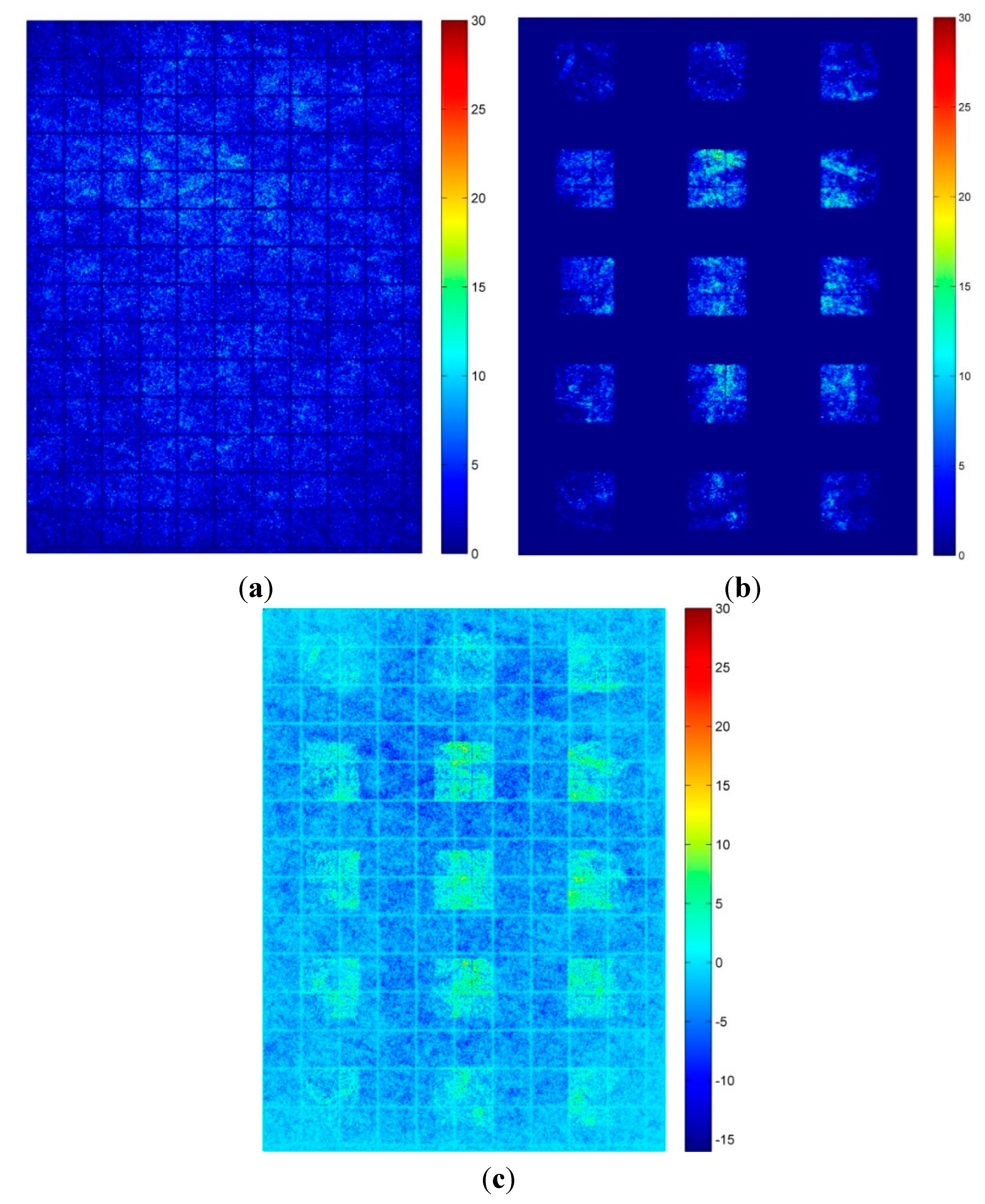
Configure the default parameters of the SIFT feature-extraction algorithm or obtain the parameters from the users, including the number of blocks in the images, which is generally the number of cell rows and columns in one image. In our experiment, the images were divided into five rows and three columns with a total 15 cells shown in the top right corner of Figure 8, and an image block was 800 × 800 pixels in the center of the image cell; as such, there are 15 blocks in one image; This division is based on demand of the von Gruber locations in the traditional aerial photogrammetry;

(2)

Calculate the sizes of the blocks and their positions in the image according to the image size and parameters;

(3)

Extract SIFT features from the blocks; calculate the weighted average of the numbers of features in the blocks as T with the Equation (3):

$$\begin{array}{l}\text{T}=\frac{{\displaystyle \sum _{\text{ib}=1}^n{H}_{ib}\times N_{ib}}}{n}\\ H=-{\displaystyle \sum _{i=0}^{L-1}{P}_i{\text{log}}_2{P}_i}\end{array}$$

(3)

where n is the number of blocks in one image; N_ib is the number of features in block ib; H_ib is the image information entropy of block ib, calculated by the second formula; P_i is the probability of gray level i(i = 0,1,…,255) in the block ib; L equals 256 in our experiment;

(4)

If the number of features in one block is less than T, then go to step (5), otherwise extraction of this block is finished, go to step (7);

(5)

Modify the parameters of the SIFT feature-extraction algorithm in accordance with the current number of points, then go to step (6).

(6)

Redo the extraction on the image block with the new parameters, and continue to step (7) whether the number of features is less than T or not;

(7)

Finish extracting for the image.

In this improved feature extraction algorithm, feature extraction for each image block is not performed more than twice. Before and after the average is calculated, these blocks in one image are processed in parallel using the multi-threaded technique.

Block matching strategy: The block matching strategy of coarse-to-fine is adopted to match the feature points extracted by the BAoSIFT feature extraction algorithm. This strategy is showed in Figure 6. At first, the coarse matching operates the resampled images of the size less than 1000 × 1000 pixels. SIFT Features are extracted and matched from the resampled images to obtain the pixels mapping parameters to judge the overlap of blocks on the original image pair. Second, unlike the strategy to match the features in the whole image presented in the paper of Huo [30], we just extract features from the blocks distributed as von Gruber regions in the original corrected image with the BAoSIFT Feature Extracting method and search initial match correspondences between the overlapped block pair. Then, RANSAC and geometric constraints, homography geometry in our BA experiment, are combined to eliminate false match correspondences in the overlapped block pair. These operations of BAoSIFT feature extracting and correspondences matching are repeated on the block until all the overlapped blocks in one image pair have been processed. Finally, a simple geometric constraint, actually the 3σ rule by counting the parallaxes of the correspondences in the BA experiment, is used to perform overall optimization and to remove false match points in non-overlapping blocks obtained due to repeating textures.

Simple multi-view verification: To each correspondence, the same ID is assigned, and this ID is also assigned to other points in other images which meet the matching requirements with either of this pair of correspondences. The actual procedure may be complex; Figure 9 shows a simple case of five images, Photo 1 to Photo 5. The links in Figure 9 indicate the correct corresponding points after matching constraint validation. Then IDs are assigned to these correspondence pairs, like the numbers in the figure. The ID 2 points appear in two images, ID 5 and ID 6 points are four overlapping tie points, and the others are three overlapping tie points. Although this method is simple, it is very practical in our experiment. The overlap of each correspondence, which is the number of each ground point’s visibility in the images, is counted simultaneously. After all matched points are assigned ID, low overlap points are deleted. In our experiment, points with less than three-lap along the flight direction are not exported for BA. We adopt this operation based on the fact that points with two-lap along the flight direction, like point with ID 2, are only used for the relative orientation, while high overlap tie points can be used for continuous relative orientation, and the points with two-lap across the flight can be used for connecting adjacent flight strips. This fact makes the geometric network of BA more stable.

Figure 9. Simple multi-view matching algorithm.

Figure 9. Simple multi-view matching algorithm.

After the tie-point connection procedure above, a large number of precise image tie points can be obtained for BA.

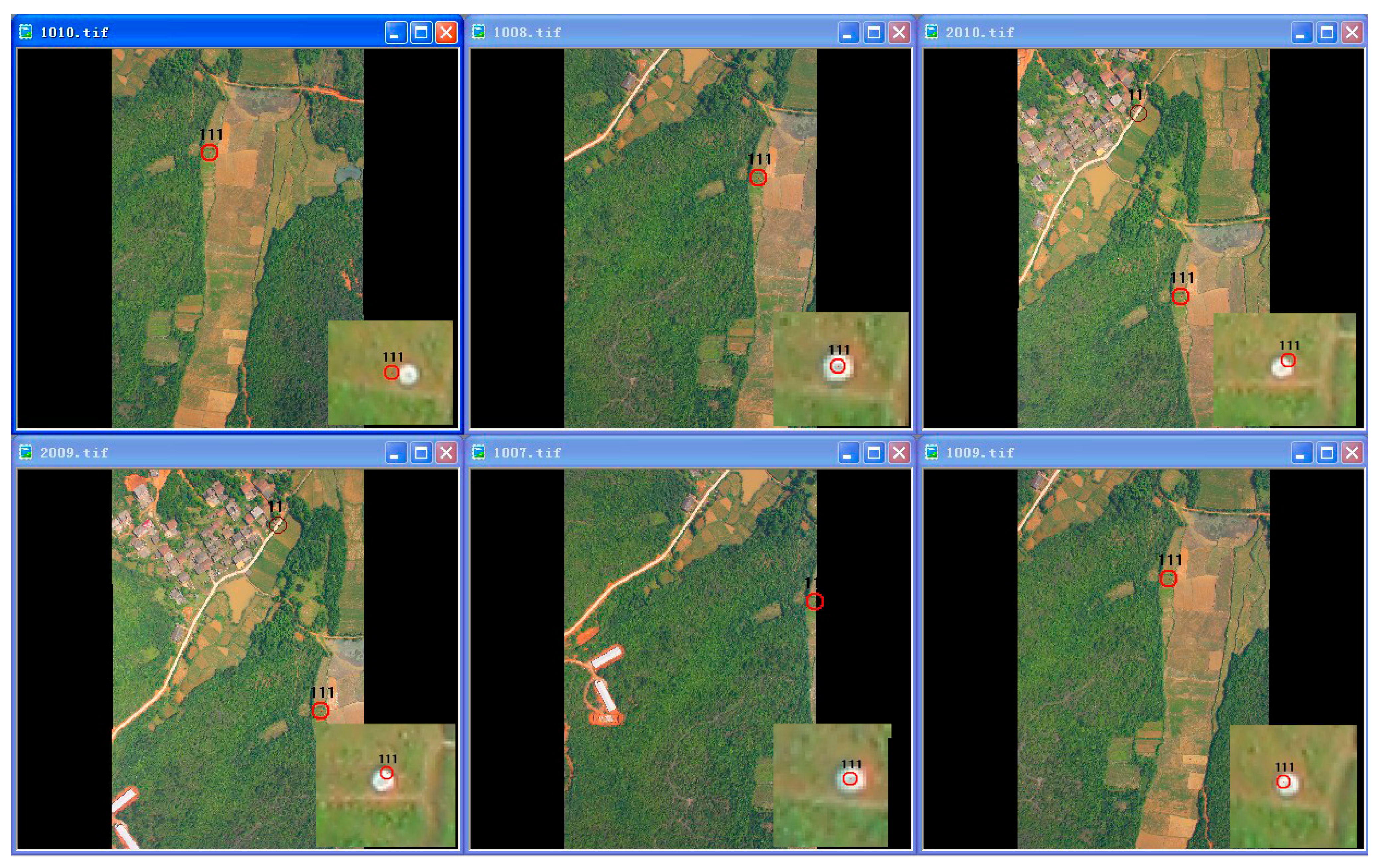
4.4. Ground Control Point Prediction

The Ground Control Point Prediction can be expressed by Equation (4):

$$\left[\begin{array}{c}{X}_2\\ Y_2\\ 1\end{array}\right]=M\left[\begin{array}{c}{X}_1\\ Y_1\\ 1\end{array}\right]$$

(4)

where M is the transformation. It is a 3 × 3 matrix, and it is invertible.

If the transformation is precise, the calculation can be continuous. The M matrices between every two overlapping images can be calculated using the image-matching result, and then the corresponding points in other images can be predicted.

To deal with UAV images with POS data, the loss of some GCPs in certain images can be reduced thanks to the combination of POS data and matching results, in this way, the efficiency can be improved. The visibility of GCPs in an image can be estimated with POS data using the method described in Section 4.1. Moreover, the transformation obtained by the matching results also contributes to the estimate and can map to the GCP positions in other images. As Figure 10 shows, once the GCP labeled “111” in the image “1008.tif” (the middle one in the top row in the figure) has been identified, then its corresponding points in other images (in the same flight strip, 1007.tif, 1009.tif, 1010.tif; in the above adjacent flight strip, 2009.tif, 2010.tif) around the current image can be predicted automatically according to the POS data and the transformation. The lower right corner of each image is the enlarged picture. This enlarged picture shows that the predictions in the current and adjacent flight strips are both relatively accurate. Then, the point is manually moved to the center of the white circle, and the identification is finished. This prediction contributes to the efficiency of identification.

Figure 10. Rapid control-point prediction based on POS data and SIFT matching.

Figure 10. Rapid control-point prediction based on POS data and SIFT matching.

The GCP prediction method proposed in this paper does not require more than four control points which are necessary if the back-intersection is used to predict the GCP. This offers an alternative to reduce the workload of identifying GCPs.

4.5. Bundle Adjustment

To perform bundle adjustment, the GCPs and their identical image positions, and the matching tie points in the images obtained by the algorithms as described in Section 4.3 and Section 4.4 are organized in the PATB input file format. Then, the PATB takes on the task of bundle adjustment. As the images are corrected for distortion, there is no need to use the self-calibrating bundle adjustment. The PATB software provides the EOs of each image and the tie points’ geodetic coordinates.

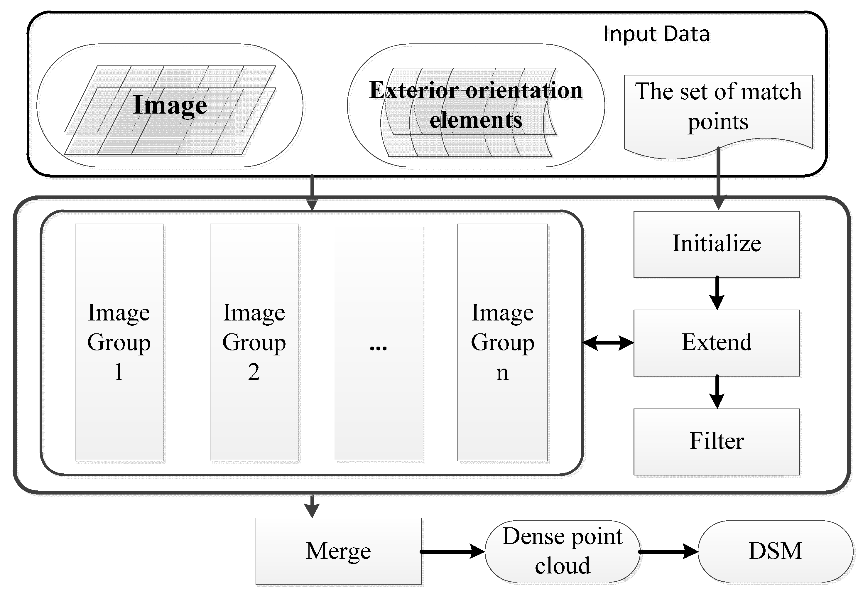
4.6. Dense Matching and Generation of Digital Surface Models (DSM) and Digital Orthophoto Maps (DOM)

DSM can be generated by dense image matching or by human–computer interaction. The points obtained by human interaction are sparse and need further manual editing to generate accurate DSM. The PMVS (Patch-based Multi-view Stereo Software) [31] was improved to perform dense matching in this research. As PMVS on a single computer cannot handle many images at one time, the images are grouped, and each group of images is used with PMVS to generate a dense point cloud and then merge these point clouds into a point cloud of the entire survey area. The first step of PMVS is to generate seed points by matching Harris and Difference-of-Gaussian (DOG) features. This time-consuming step is omitted, and the match points obtained as described in Section 4.3 are used as seed points after initialized, followed by extensions and filters as the second and third step of PMVS to acquire the dense point cloud. The dense point cloud is interpolated to generate the DEM. The procedures are shown in Figure 11. Then, orthophotos are obtained by orthorectification with the DEM and the corrected images, and all the orthophotos mosaic to form a single DOM.

Figure 11. Procedure for dense matching.

Figure 11. Procedure for dense matching.

4.7. Three-Dimensional Visualization

The last task is to show the DEM and DOM, both are 0.1 m high-resolution. There are several free softwares for 3D visualization of DEM and DOM, such as World Wind, Virtual Terrain Project and osgEarth. We adopt the World Wind which is an open-source software package developed by the United States National Aeronautics and Space Administration (NASA). World Wind can manage multi-source geospatial data, their distribution, and their three-dimensional visualization [32] and solves the vital problems of seamless integration, management, and highly efficient display of multi-source geospatial data (DOM, DEM, KML) and other third-party data.

This paper achieves three-dimensional visualization by adapting the DEM and DOM to the World Wind data model. The images and elevation data that World Wind supports are organized as a pyramidal model, and therefore we develop a data-processing tool to cut DEM and DOM into slices and blocks and transform these tiles to the file format of World Wind’s data model.

5. Results and Discussion

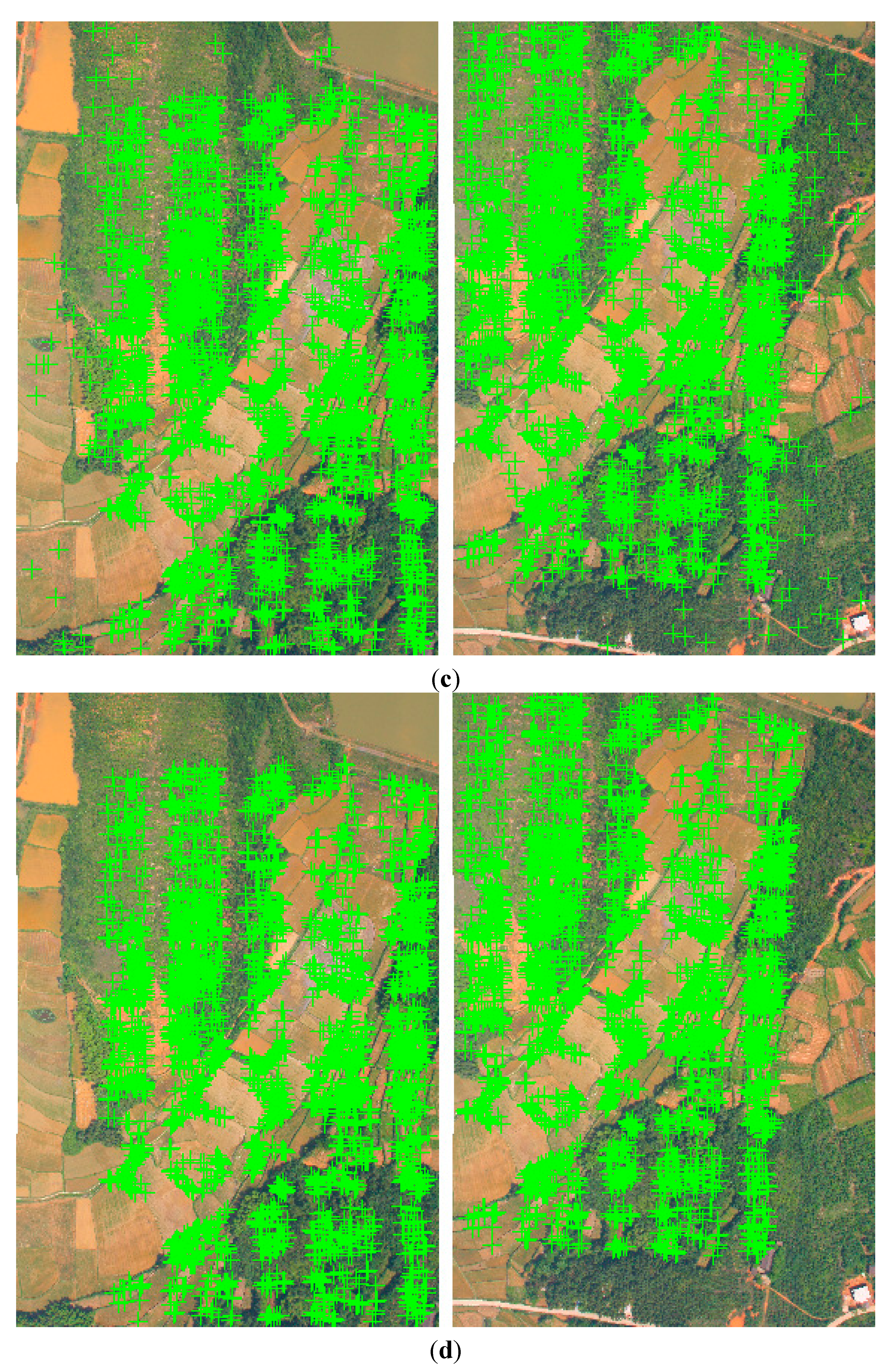
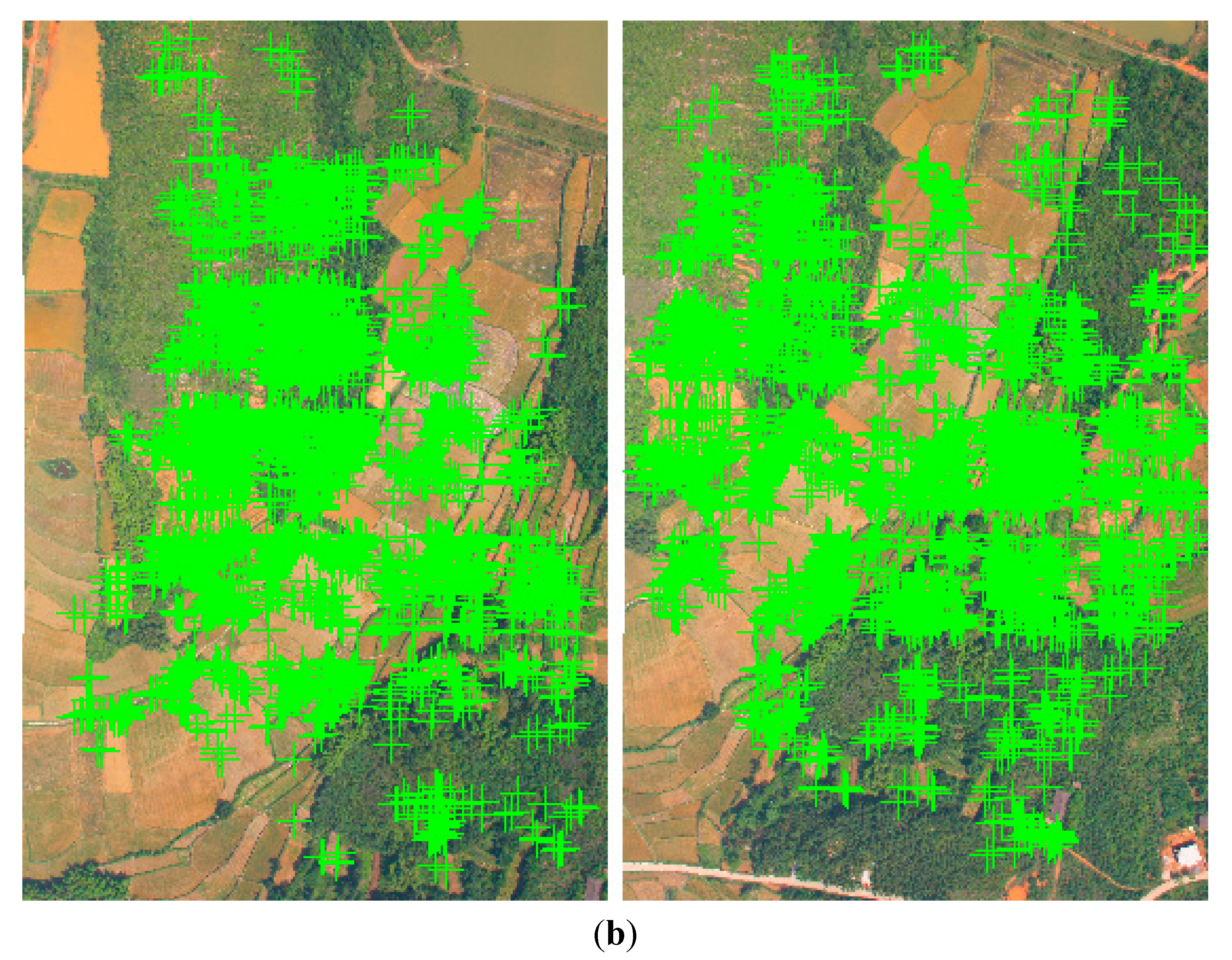
Low-altitude UAV images and GCPs were used as sources for experiments on the proposed approaches to photogrammetric processing. The operation of selecting gross error points through human–computer interaction during AT is not included in the experiment. Instead, matching operation for tie points are directly input for bundle adjustment to obtain EOs. The matching algorithm is discussed, the precision of AT (squared error), the 3D coordinates of matched tie points and dense point cloud, DEM, and DOM are also displayed in this section.

5.1. Image Matching

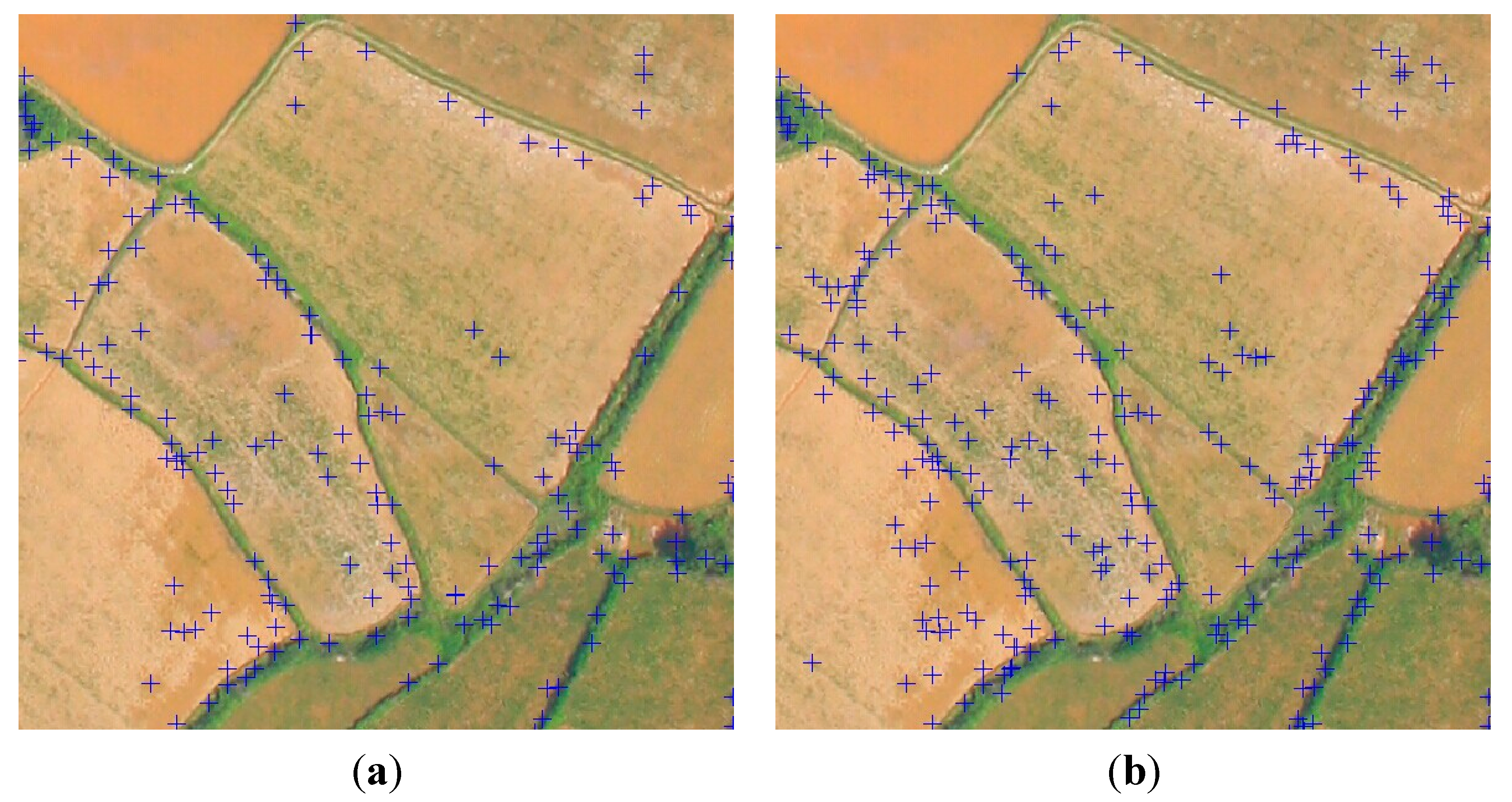
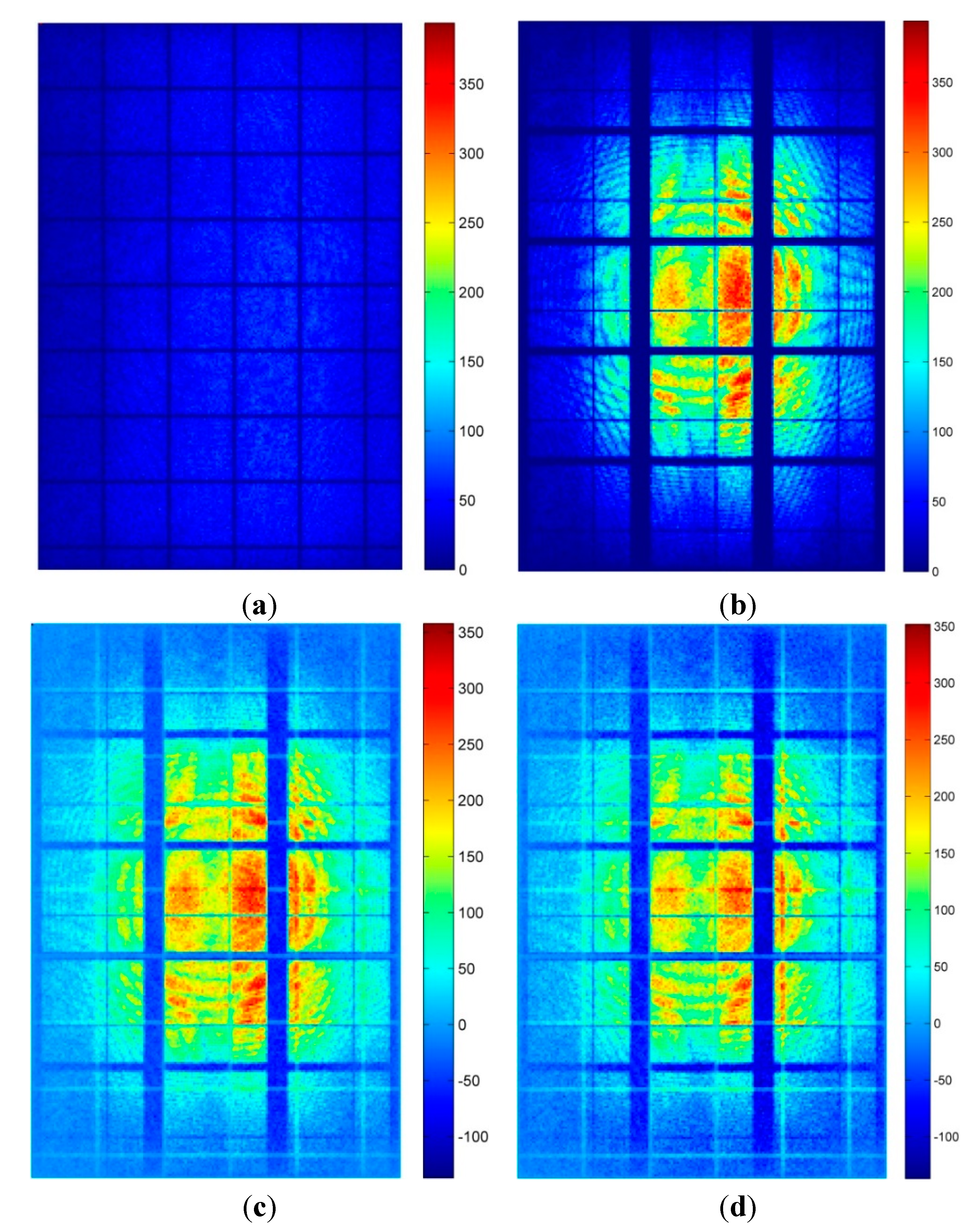
5.1.1. Efficiency and Distribution of Features

Given the same size of the input images, the performance of feature extraction is mainly determined by the block size, and this relation can be measured quantitatively. In this experiment, we choose the first typical image in Figure 3 as the put image to compare the performance and number of features extracted by the original SIFT, BAoSIFT, and BAoSIFT MT, short for BAoSIFT accelerated by multi-thread, as shown in Table 2. As the original SIFT has the problem of large memory requirement and computational complexity, we extract features in blocks of the input image in the experiment. At the same time, we get different numbers from different block sizes without considering the impact of edge, because the edge leads to the problem that more blocks and more pixels are ignored to extract features on the edges of blocks. The experiment shows the best compromise is achieved when the block size is 512 × 512, considering the time and number of features. We also find that this comparison of BAoSIFT and BAoSIFT MT demonstrates the advantages of parallel multi-thread in improving the efficiency, despite the same numbers of their features. Moreover, the improved BAoSIFT algorithm really increases the number of features. The comparison in Figure 12 shows the advantage of the BAoSIFT in the spatial distribution of the extracted points over the original SIFT algorithm.

Table 2. Comparison of SIFT to BAoSIFT.

BlockSize	SIFT		BAoSIFT		BAoSIFT MT
	Time (ms)	Number of Features	Time (ms)	Number of Features	Time (ms)
64 × 64	5007	9925	8018	12,749	2340
128 × 128	5054	12,203	8053	15,037	2424
256 × 256	5504	13,594	8081	16,606	2605
512 × 512	5679	14,209	8346	16,951	2659
1024 × 1024	5959	14,628	8736	17,635	2715

Table 2. Comparison of SIFT to BAoSIFT.

BlockSize	SIFT		BAoSIFT		BAoSIFT MT
	Time (ms)	Number of Features	Time (ms)	Number of Features	Time (ms)
64 × 64	5007	9925	8018	12,749	2340
128 × 128	5054	12,203	8053	15,037	2424
256 × 256	5504	13,594	8081	16,606	2605
512 × 512	5679	14,209	8346	16,951	2659
1024 × 1024	5959	14,628	8736	17,635	2715

Figure 12. Features are extracted from the first typical image of Figure 3. (a) The features extracted by the original SIFT in the center of the experimental image; (b) the features extracted by BAoSIFT; both block sizes are 512 × 512.

Figure 12. Features are extracted from the first typical image of Figure 3. (a) The features extracted by the original SIFT in the center of the experimental image; (b) the features extracted by BAoSIFT; both block sizes are 512 × 512.

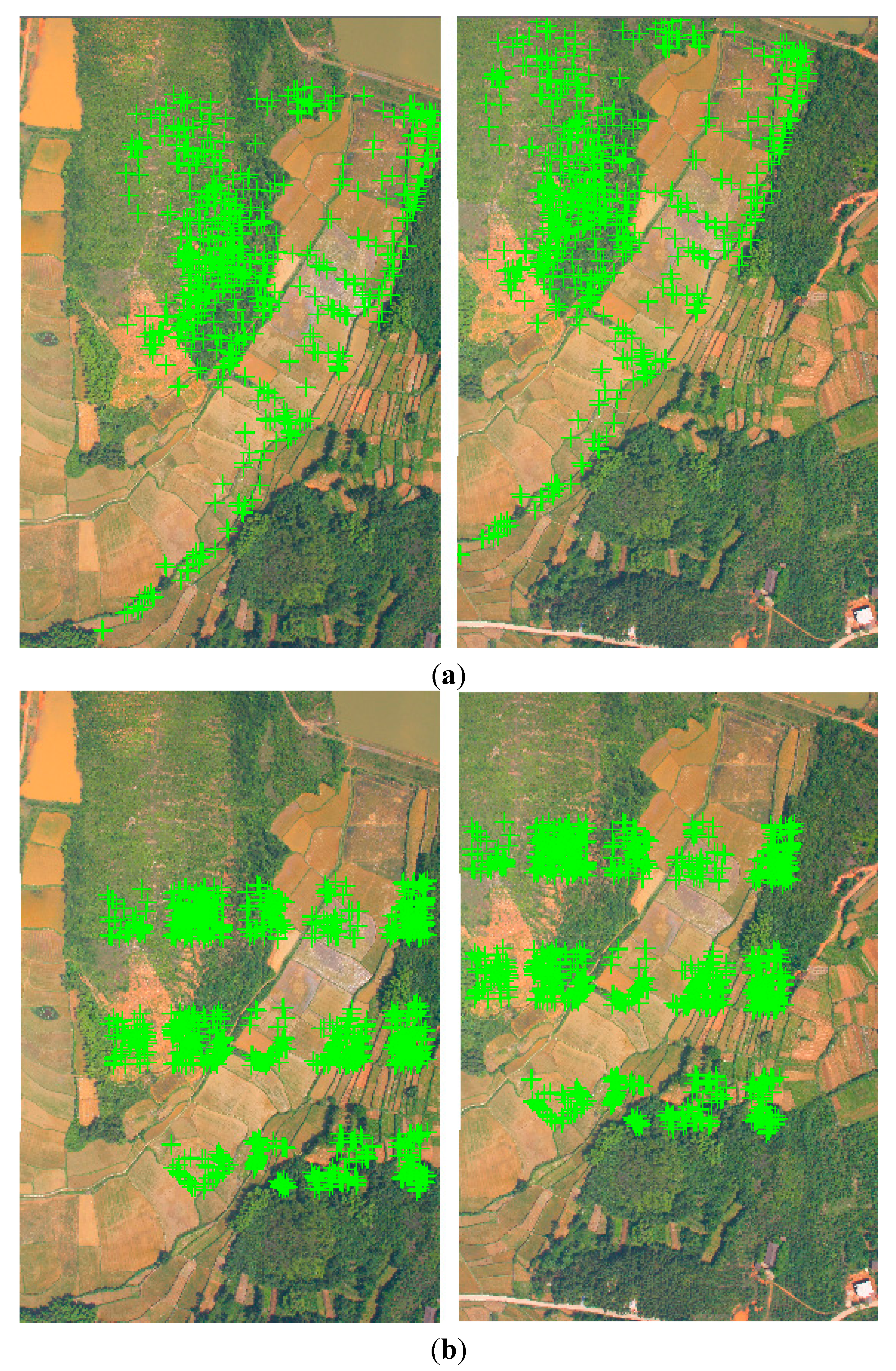
5.1.2. Feature Matching

The matching method proposed in this paper could obtain more than 1000 stable image-matching points per image pair. Table 3 and Figure 13 show matching results for the same stereo image pair using different matching strategies. In Figure 11, the crosses represent matching points. Figure 11a represents the result achieved by SIFT feature extraction and then by removing the error correspondences with the combination of RANSAC and homography constraints. The number of matching point pairs is 631; Figure 11b represents the results of the improved method presented in this paper. The images are divided into five rows and three columns, and an 800 × 800 pixels block in the center of each cell is considered as an image block to extract BAoSIFT features. All the features of the small overlapped block pairs in the image pair are matched using RANSAC and homography constraints, and finally a simple optimization of 3σ rule is performed by counting the parallaxes of the correspondences overall. This optimization deletes the correspondences with the high parallax out of range defined by three times of the standard deviation. The number of matches is 1381; Figure 11c is almost the same as Figure 11b, but does not use the small images to estimate the overlaps. The number of matches is 3845; Figure 11d is mostly identical to Figure 11c, the only difference is the optimization with constraint of epipolar geometry, and the number of matches is 3371; After manual checking, the correspondences found by Figure 11a,b,d are all determined to be correct, while error exists in Figure 11c. There are obviously errors scattered in the left part of the left image and in the right part of the right image; in addition, error correspondences exist in other places. The homography constraint is a kind of plane constraint, which means that ground objects corresponding to identical points in the image pairs should lie in the same plane. Figure 13a shows this phenomenon that there are only matched features in the low right part of the pair. The method combining RANSAC and homography constraints tries to robustly find the plane, and tries to contain the most points. However, this plane constraint limits the distribution of the matched features. While the result of epipolar geometry covers the overlapped region of the image pair, there exist errors, as shown in Figure 13c. So, the proposed method combines their virtues. Each overlapped block pair finds the plane that contains the most points. The block-matching strategy essentially obtains matching points belonging to different planes, and therefore the number of matching points is increased. Meanwhile, the partition of transforming one image to several blocks is based on the von Gruber locations. And the result is that points are distributed more evenly to cover the image with the help of epipolar constraint, which has been proved in Figure 13b–d. The step of resampled image matching for obtaining the pixels mapping parameters is beneficial to judge the overlap of blocks on original image pair. This judgment reduces the time of processing non-overlapped blocks.

Figure 13. Matching result for UAV images: (a) remove error correspondences with the combination of RANSAC and homography constraints; (b) the improved method presented in this paper; (c) does not use the small images to estimate the overlaps; (d) optimization with constraint of epipolar geometry to remove the error correspondences based on the results in (c).

Figure 13. Matching result for UAV images: (a) remove error correspondences with the combination of RANSAC and homography constraints; (b) the improved method presented in this paper; (c) does not use the small images to estimate the overlaps; (d) optimization with constraint of epipolar geometry to remove the error correspondences based on the results in (c).

Table 3 shows the time taken for different strategies. The matching efficiency of the method used in (a) is the highest, but the matching points are unevenly distributed; The time required for (b) is three times that for (a); This time is mainly used to search for matching points, but the matching points are distributed relatively evenly according to the von Gruber points; The efficiencies of (c) and (d) are almost the same, and the matching points are evenly distributed in the overlap area of the stereo pairs, but the time required is far more than for (b); Method (b) therefore represents a good compromise between efficiency and distribution of matching points.

Table 3. Efficiency of different strategy of blockwise match.

Method	a	b	c	d
Number of Correspondences	631	1381	3845	3371
Time(ms)	2558	8074	72,649	73,415

Table 3. Efficiency of different strategy of blockwise match.

Method	a	b	c	d
Number of Correspondences	631	1381	3845	3371
Time(ms)	2558	8074	72,649	73,415

Actually, as the overlap of UAV images is irregular, one image can overlap several images (more than four images). If method (b) described above is only used, one image still shares tie points with other images. Therefore, the tie points finally lying in one image still cover the full image. As shown in Figure 14, the image pair is the same one shown in Figure 13. Figure 14 also shows the difference of quantity and distribution between the matching results obtained by using method (a) and (b); Most correspondences of method (b) concentrate in the image. These tie points are vital for AT because they ensure, not only that enough redundant observations are obtained, but also that all the images are connected. This method gets all the correspondences for BA in our experiment.

Figure 14. Final results of image matching obtained by using method (a) and (b).

Figure 14. Final results of image matching obtained by using method (a) and (b).

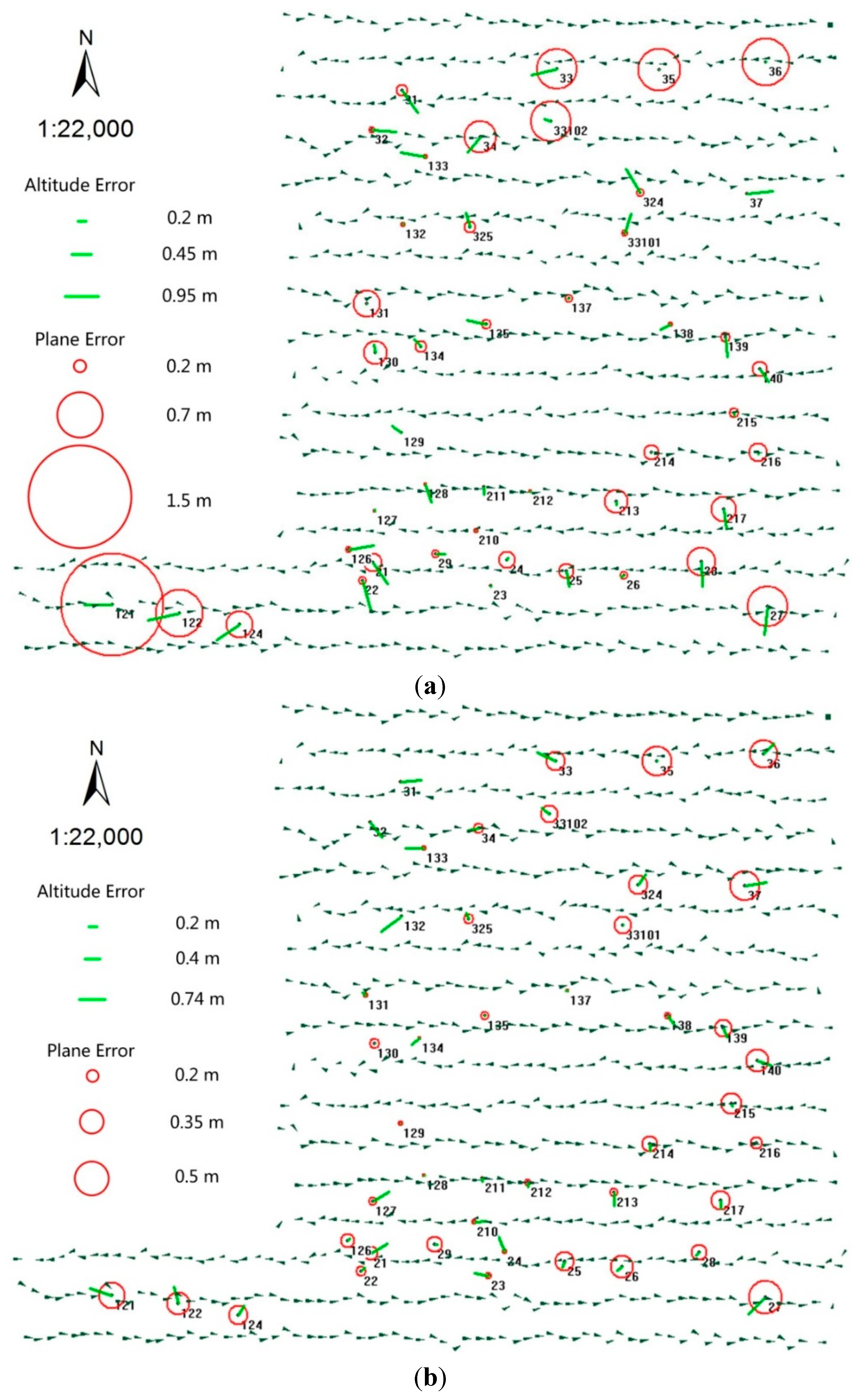
5.2. Bundle Adjustment

To evaluate fully the accuracy of the workflow proposed in this paper for low-altitude images, BA experiments with GCPs are performed with the two datasets Yangqiaodian and PDS, respectively. The free software VisualSFM [6] is adopted to compare the precision of AT. Coming from the Computer Vision community, VisualSFM is not a photogrammetric software application and does not use control points as constraints in the bundle but only for a posteriori rigid Helmert transformation (scale and geo-referencing). However, VisualSFM has been adopted for UAV and close range image orientation.

5.2.1. Yangqiaodian

Two methods are adopted to generate the tie points—the original SIFT and BAoSIFT—namely the Method (a) and (b) in Figure 13. During the procedure of both methods, features are extracted by using parallel multi-thread with the block size of 512 × 512. During the matching procedure of BAoSIFT, images are divided into five rows and three columns (15 cells), and 800 × 800 pixel block in the center of each image cell is processed. Of the 1,337,667 tie points with the overlap, more than two are finally obtained, while the original SIFT obtains 896,495 tie points without two-lap points being discarded. After identifying the GCPs and BA by PATB, the AT results were as displayed in Table 4. The SIFT and BAoSIFT approaches use the same GCPs, check points and the setup of BA. The root-mean-square values (RMS) of GCPs and check points of results of the BAoSIFT is better than those of SIFT. On the whole, Table 4 shows advantages of BAoSIFT over SIFT in the RMSs of GCPs and check points. The RMSs of GCPs and check points in Table 4 demonstrate the rationality of the successful result, compared to the original SIFT method. In order to compare the results of AT, the geometrical corrected images and the GCPs are fed to the free software VisualSFM, which uses SIFT for feature extracting and matching as well. After exhaustive pair-matching (n × (n − 1)/2, n is the number of images) and BA, the free software VisualSFM obtains the oriented results and 3D points corresponding to these tie points. In particular, the tie points with at least three-lap are required for BA of VisualSFM. It is worth noting that the statistical results from VisualSFM are processed by space intersection with multi-image due to the lack of statistical reports in object space provided by the software. At the same time, the software PATB prompts that it cannot process the input image points delivered by VisualSFM when we use these matched tie points. Table 4 shows the lower precision obtained by VisualSFM than that of SIFT and BAoSIFT.

Table 4. Precision of AT in the Yangqiaodian area.

Method	Control Points (m)						Check Points (m)
Evaluation	Max (ΔX)	Max (ΔY)	Max (ΔZ)	RMS (X)	RMS (Y)	RMS (Z)	Max (ΔX)	Max (ΔY)	Max (ΔZ)	RMS (X)	RMS (Y)	RMS (Z)
SIFT (a)	1.51	0.61	0.97	0.32	0.24	0.54	0.57	0.37	0.83	0.23	0.22	0.51
BAoSIFT (b)	0.42	0.38	0.74	0.17	0.17	0.38	0.32	0.26	0.55	0.16	0.17	0.36
VisualSFM	1.21	0.98	1.33	0.65	0.56	0.82	1.42	1.01	1.46	0.78	0.68	0.91

Table 4. Precision of AT in the Yangqiaodian area.

Method	Control Points (m)						Check Points (m)
Evaluation	Max (ΔX)	Max (ΔY)	Max (ΔZ)	RMS (X)	RMS (Y)	RMS (Z)	Max (ΔX)	Max (ΔY)	Max (ΔZ)	RMS (X)	RMS (Y)	RMS (Z)
SIFT (a)	1.51	0.61	0.97	0.32	0.24	0.54	0.57	0.37	0.83	0.23	0.22	0.51
BAoSIFT (b)	0.42	0.38	0.74	0.17	0.17	0.38	0.32	0.26	0.55	0.16	0.17	0.36
VisualSFM	1.21	0.98	1.33	0.65	0.56	0.82	1.42	1.01	1.46	0.78	0.68	0.91

It is well known that the result of AT is affected by many factors, such as the accuracy and distribution of GCPs, the number and distribution of tie points, overlaps between images, the base-to-height ratio. In this study, the only difference is the matching method, which results in different overlap, numbers and distribution of tie points. Therefore, we add the numbers of tie points in all the images as follows. As the size of image is 2848 × 4272, we divide the image into 178 × 267 grids with the size of 16 × 16 pixels (16 is their greatest common divisor). Then, we count the number of tie points within each grid. The statistical results are shown in Figure 15, which shows the number of tie points of each grid. The present block edges (blue grid lines) demonstrated in Figure 15 have no tie points attributed to the implementation of Feature Extracting algorithm designed for the block size 512 × 512. It is worth noting that the original SIFT method is also based on the same block-multi-thread strategy with BAoSIFT to avoid the different processings. Except for the aforementioned edges in Figure 15a,b, the tie points resulted from the BAoSIFT method present a higher level of coverage compared with those by the original SIFT method shown in Figure 15c. This can be confirmed by the positive results obtained based on the reduction of BAoSIFT and SIFT in Figure 15c. Even when we increase the point size of Figure 15a by 1.5 times, the result in Figure 15d still indicates the same conclusion as Figure 15c. Figure 15 proves the advantages of the BAoSIFT method in characterizing the overlap, number and distribution of the tie points over the SIFT method. This is also the reason that BAoSIFT gains higher precision of BA compared with the SIFT method.

The error distribution of GCPs and check points will show the rationality once more. Figure 16 shows the GCPs’ error distribution of the result of SIFT and BAoSIFT. Lines at each point represent altitude error, the orientation of the lines represents the orientation of the plane error (atan(dy/dx)), and the circles represent the values of the plane error. The GCPs with relatively large errors are mostly distributed on the edge of the area, shown in both results of Figure 16. The upper left and the bottom parts in both of the two figures have large features. This similarity of distribution of error shows the two methods’ rationality.

Figure 15. The comparison of BAoSIFT and SIFT methods in generating tie points in the study area of Yangqiaodian. (a) SIFT; (b) BAoSIFT; (c) BAoSIFT-SIFT; (d) BAoSIFT-1.5 × SIFT.

Figure 15. The comparison of BAoSIFT and SIFT methods in generating tie points in the study area of Yangqiaodian. (a) SIFT; (b) BAoSIFT; (c) BAoSIFT-SIFT; (d) BAoSIFT-1.5 × SIFT.

The PATB software obtains 3D coordinates for the ground points corresponding to the tie points, as shown in Figure 17. This figure shows the distribution of the ground points corresponding to the matched image features acquired by BAoSIFT. This figure also shows these points cover the experimental area, and there are no large gaps except for water regions.

Figure 16. Error distribution of GCPs and check points in Yangqiaodian. (a) SIFT; (b) BAoSIFT.

Figure 16. Error distribution of GCPs and check points in Yangqiaodian. (a) SIFT; (b) BAoSIFT.

Figure 17. 3D point cloud for the Yangqiaodian area.

Figure 17. 3D point cloud for the Yangqiaodian area.

5.2.2. PDS

To further demonstrate the BAoSIFT algorithm, three methods are adopted to generate the tie points, the original SIFT, BAoSIFT, namely the Method (a) and (b) in Figure 13 of the manuscript, and VisualSFM. The matching procedure of BAoSIFT includes the same operations as those in the experimental dataset of Yangqiaodian: images are divided into five rows and three columns (15 cells), and an 800 × 800 pixel block in the center of each image cell is processed. In total, 16,244 tie points with the overlap of more than 2 are finally obtained by BAoSIFT, while 100,482 tie points are acquired by the original SIFT method. After identifying the GCPs and BA by PATB, the AT results are revealed in Table 5. The SIFT and BAoSIFT approaches use the same GCPs, check points and the configurations of BA. VisualSFM shares the same GCPs and check points with the other two. The root-mean-square values (RMS) of GCPs and check points of results of the BAoSIFT are better than those of SIFT and VisualSFM. VisualSFM obtained the lowest precision. We also use PATB to bundle-adjust the tie points generated by VisualSFM with the same GCPs, check points and the configurations of BA as the SIFT and BAoSIFT approaches do. Table 5 shows the exhaustive pair-matching of VisualSFM, (n × (n − 1)/2, n is the number of images) achieves better precision than the original SIFT in our manuscript, but worse precision than BAoSIFT. The difference between the three approaches also results from the different overlap, numbers and distribution of tie points.

Table 5. Precision of AT in the PDS area.

Method	Control Points (m)						Check Points (m)
	Max			Std			Max			Std
	X	Y	Z	X	Y	Z	X	Y	Z	X	Y	Z
SIFT	0.140	0.114	0.657	0.035	0.032	0.189	0.142	0.052	0.437	0.048	0.025	0.167
BAoSIFT	0.135	0.070	0.192	0.021	0.019	0.042	0.132	0.046	0.231	0.039	0.019	0.070
VisualSFM	0.530	0.640	0.810	0.180	0.240	0.430	0.470	0.610	0.980	0.160	0.190	0.520
VisualSFM-PATB	0.149	0.056	0.842	0.025	0.024	0.140	0.139	0.055	0.589	0.038	0.027	0.159

Table 5. Precision of AT in the PDS area.

Method	Control Points (m)						Check Points (m)
	Max			Std			Max			Std
	X	Y	Z	X	Y	Z	X	Y	Z	X	Y	Z
SIFT	0.140	0.114	0.657	0.035	0.032	0.189	0.142	0.052	0.437	0.048	0.025	0.167
BAoSIFT	0.135	0.070	0.192	0.021	0.019	0.042	0.132	0.046	0.231	0.039	0.019	0.070
VisualSFM	0.530	0.640	0.810	0.180	0.240	0.430	0.470	0.610	0.980	0.160	0.190	0.520
VisualSFM-PATB	0.149	0.056	0.842	0.025	0.024	0.140	0.139	0.055	0.589	0.038	0.027	0.159

In this experimental dataset, we also compare the distribution and overlap of tie points using the same method that we divide the images into grids with the size of 16 × 16 pixels. Then, we summarize the numbers of tie points within the same grid. The statistical results are displayed in Figure 18, which demonstrates that BAoSIFT obtains many more tie points than SIFT at von Gruber locations. This is the key difference of the two methods, which leads to the different results from BA.

Figure 18. The comparison of BAoSIFT and SIFT methods in generating tie points in the study area of PDS. (a) SIFT; (b) BAoSIFT; (c) BAoSIFT–SIFT.

Figure 18. The comparison of BAoSIFT and SIFT methods in generating tie points in the study area of PDS. (a) SIFT; (b) BAoSIFT; (c) BAoSIFT–SIFT.

Figure 19 shows the GCPs’ error distribution of the results from SIFT and BAoSIFT. The error distribution of the two approaches share some features that most of the GCPs and check points have little error, and the plane error of two points in the center is relatively large.

Figure 19. Error distribution of GCPs and check points in PDS. (a) SIFT; (b) BAoSIFT.

Figure 19. Error distribution of GCPs and check points in PDS. (a) SIFT; (b) BAoSIFT.

5.3. 3D Visualization of Digital Elevation Model (DEM) and Digital Orthophoto Maps (DOM)

This experiment feeds the PMVS software with matched points to obtain a dense point cloud, which is used to generate a DSM. Then, orthophotos are produced with the point cloud or the DEM and the images corrected by the method described in Section 4.2. All the orthophotos are then merged into a single DOM. Figure 20a shows the dense 3D point cloud obtained from two adjacent images in Yangqiaodian, and Figure 20b shows the DOM obtained from the dense point cloud and the two corresponding adjacent corrected images.

With the help of improvements to the NASA World Wind open-source software, a three-dimensional display could finally be realized, as the 3D scene of Yangqiaodian area shown in Figure 21. All the corrected images are grouped to calculate the dense point cloud, and then these point clouds are merged into one point cloud for generating the DSM. The whole DEM dataset of the area is obtained by filtering the DSM. All of these corrected images are orthorectified into DOM. The DEM and DOM of the area are overlapped to form the visual 3D scene, shown in Figure 21.

Figure 20. From dense point cloud to orthophoto: (a) Colorful dense point cloud generated by PMVS; (b) Orthophoto generated based on dense point cloud and corrected image.

Figure 20. From dense point cloud to orthophoto: (a) Colorful dense point cloud generated by PMVS; (b) Orthophoto generated based on dense point cloud and corrected image.

6. Conclusions

Experimental results show that the method proposed in this paper is effective and feasible for UAV images. With the proposed methods, localization and orientation of UAV images could be achieved with low cost. It can be concluded that the proposed methods have great potential in surveying and mapping and emergency disaster response.

The automated strip arrangement described in the paper is able to process rough flight data and to calculate the FOV of images. Thus, overlaps and connections can be obtained, which save the matching time for stereo image pairs with large rotation angles and irregular overlaps and reduce the matching error effectively. Based on the consistency of the distortion of each image, correction could be carried out by means of the lookup-table technique. Furthermore, the efficiency of distortion correction can be improved significantly by OpenMP. Large quantities of evenly distributed matching points could be found from UAV image pairs with the BAoSIFT. With the GCP prediction method proposed in this paper, the identification workload can be reduced significantly. The results of the BAoSIFT matching algorithm and the GCP coordinates are output directly to PABT to carry out the AT calculations, which implement automatic AT processing for the large-rotation, small-format images acquired by low-altitude UAVs. DSM and DOM can be obtained after orientation to provide 3D visualization on World Wind.

Figure 21. 3D visualization of Yangqiaodian with the help of improved World Wind.

Figure 21. 3D visualization of Yangqiaodian with the help of improved World Wind.

Although multithread technology has been used in this research to improve the efficiency of SIFT feature extraction, the computing time of SIFT is huge, and the efficiency of SIFT feature extraction still needs to be improved. Improving the extraction and the matching algorithm combined with other features will be a focus of future research. The integration of rough flight data into the aerial bundle adjustment to make full use of flight data and improve efficiency is also an important future research topic. The rule of affect for the distribution of tie points on the BA is yet to be determined by researchers.

References

1. Zhang, Y.; Xiong, J.; Hao, L. Photogrammetric processing of low-altitude images acquired by unpiloted aerial vehicles. Photogramm. Rec. 2011, 26, 190–211. [Google Scholar] [CrossRef]
2. Remondino, F.; Barazzetti, L.; Nex, F.; Scaioni, M.; Sarazzi, D. UAV photogrammetry for mapping and 3d modeling–current status and future perspectives. In Proceedings of the International Conference on Unmanned Aerial Vehicle in Geomatics (UAV-g), Zurich, Switzerland, 14–16 September 2011.
3. Büyüksali̇h, G.; Li, Z. Practical experiences with automatic aerial triangulation using different software packages. Photogramm. Rec. 2003, 18, 131–155. [Google Scholar] [CrossRef]
4. Laliberte, A.S.; Herrick, J.E.; Rango, A.; Winters, C. Acquisition, orthorectification, and object-based classification of unmanned aerial vehicle (UAV) imagery for rangeland monitoring. Photogramm. Eng. Remote Sens. 2010, 76, 661–672. [Google Scholar] [CrossRef]
5. Pierrot-Deseilligny, M.; Luca, L.D.; Remondino, F. Automated image-based procedures for accurate artifacts 3d modeling and orthoimage generation. In Proceedings of the 23th International CIPA Symposium, Prague, Czech Republic, 12–16 September 2011.
6. Visualsfm: A Visual Structure from Motion System. Available online: http://ccwu.me/vsfm/ (accessed on 17 February 2015).
7. Deseilligny, M.P.; Clery, I. Apero, an open source bundle adjusment software for automatic calibration and orientation of a set of images. In Proceedings of the International Archives of Photogrammetry, Remote Sensing and Spatial Information Sciences, Trento, Italy, 2–4 March 2011; Volume 38.
8. Snavely, N.; Seitz, S.M.; Szeliski, R. Modeling the world from internet photo collections. Int. J. Comput. Vis. 2007, 80, 189–210. [Google Scholar] [CrossRef]
9. Nex, F.; Remondino, F. UAV for 3d mapping applications: A review. Appl. Geomat. 2014, 6, 1–15. [Google Scholar] [CrossRef]
10. Barazzetti, L.; Scaioni, M.; Remondino, F. Orientation and 3D modelling from markerless terrestrial images: Combining accuracy with automation. Photogram. Rec. 2010, 25, 356–381. [Google Scholar] [CrossRef]
11. Barazzetti, L.; Remondino, F.; Scaioni, M.; Brumana, R. Fully automatic UAV image-based sensor orientation. In Proceedings of the ISPRS Commission I Mid-Term Symposium “Image Data Acquisition-Sensors & Platforms”, Calgary, AB, Canada, 15–18 June 2010.
12. Haala, N.; Cramer, M.; Weimer, F.; Trittler, M. Performance test on UAV-based photogrammetric data collection. In Proceedings of the International Conference on Unmanned Aerial Vehicle in Geomatics (UAV-g), Zurich, Switzerland, 14–16 September 2011; Volume XXXVIII-1/C22.
13. Pollefeys, M.; Gool, L.V. From images to 3d models. In Communications of the ACM-How the Virtual Inspires the Real; ACM: New York, NY, USA, 2002; pp. 50–55. [Google Scholar]
14. Hao, X.; Mayer, H. Orientation and auto-calibration of image triplets and sequences. Int. Arch. Photogramm. Remote Sens. Spat. Inf. Sci. 2003, 34, 73–78. [Google Scholar]
15. Nister, D. Automatic passive recovery of 3d from images and video. In Proceedings of the 2nd International Symposium on 3D Data Processing, Visualization and Transmission, Thessaloniki, Greece, 6–9 September 2004; pp. 438–445.
16. Vergauwen, M.; Gool, L.V. Web-based 3d reconstruction service. Mach. Vis. Appl. 2006, 17, 411–426. [Google Scholar] [CrossRef]
17. Barazzetti, L.; Remondino, F.; Scaioni, M. Automation in 3d reconstruction: Results on different kinds of close-range blocks. In Proceedings of the ISPRS Commission V Mid-Term Symposium “Close Range Image Measurement Techniques”, Newcastle upon Tyne, UK, 21–24 June 2010.
18. Lowe, D.G. Object recognition from local scale-invariant features. In Proceedings of the International Conference on Computer Vision, Corfu, Greece; 1999; pp. 1150–1157. [Google Scholar]
19. Lowe, D.G. Distinctive image features from scale-invariant keypoints. Int. J. Comput. Vis. 2004, 60, 91–110. [Google Scholar] [CrossRef]
20. Fischler, M.A.; Bolles, R.C. Random sample consensus: A paradigm for model fitting with applications to image analysis and automated cartography. Gr. Image Process. 1981, 24, 381–395. [Google Scholar]
21. Förstner, W. A feature based correspondence algorithm for image matching. Int. Arch. Photogramm. Remote Sens. Spat. Inf. Sci. 1986, 26, 150–166. [Google Scholar]
22. Harris, C.; Stephens, M. A combined corner and edge detector. In Proceedings of the Fourth Alvey Vision Conference, Manchester, UK; 1988; pp. 147–151. [Google Scholar]
23. Laliberte, A.S.; Winters, C. A procedure for orthorectification of sub-decimeter resolution imagery obtained with an unmanned aerial vehicle (UAV). In Proceedings of the ASPRS 2008 Annual Conference, Portland, OR, USA, 28 April–2 May 2008.
24. Rosten, E.; Drummond, T. Machine learning for high-speed corner detection. In Proceedings of the 9th European conference on Computer Vision(ECCV’06), 7–13 May 2006; pp. 430–443.
25. k2-photogrammetry. Patb. Available online: http://www.k2-photogrammetry.de/products/patb.html (accessed on 17 February 2015).
26. SWDC Digital Aerial Camera. Available online: http://www.jx4.com/en/home/home/tjcp/SWDC_Digital/2014/0326/422.html (accessed on 17 February 2015).
27. National Administration of Surveying, Mapping and Geoinformation of China (NASMG). Specifications for Field Work of Low-Altitude Digital Aerophotogrammetry; NASMG: Beijing, China, 2010; CH/Z 3004-2010. [Google Scholar]
28. OpenMP.org. Openmp. Available online: http://openmp.org/wp/ (accessed on 17 February 2015).
29. McGlone, C. Manual of Photogrammetry, 6th ed.; ASPRS: Bethesda, MD, USA, 2013. [Google Scholar]
30. Huo, C.; Pan, C.; Huo, L.; Zhou, Z. Multilevel SIFT matching for large-size VHR image registration. IEEE Geosci. Remote Sens. Lett. 2012, 9, 171–175. [Google Scholar] [CrossRef]
31. Furukawa, Y.; Ponce, J. Accurate, dense, and robust multiview stereopsis. IEEE Trans. Pattern Anal. Mach. Intell. 2010, 32, 1362–1376. [Google Scholar] [CrossRef] [PubMed]
32. Bell, D.G.; Kuehnel, F.; Maxwell, C.; Kim, R.; Kasraie, K.; Gaskins, T.; Hogan, P.; Coughlan, J. NASA world wind: Opensource gis for mission operations. In Proceedings of the Aerospace Conference, Big Sky, MT, UAS, 3–10 March 2007; pp. 1–9.