
Mapping Natura 2000 Habitat Conservation Status in a Pannonic Salt Steppe with Airborne Laser Scanning


Abstract
:
1. Introduction
State of the Art in N2000 Conservation Status Assessment
2. Objectives
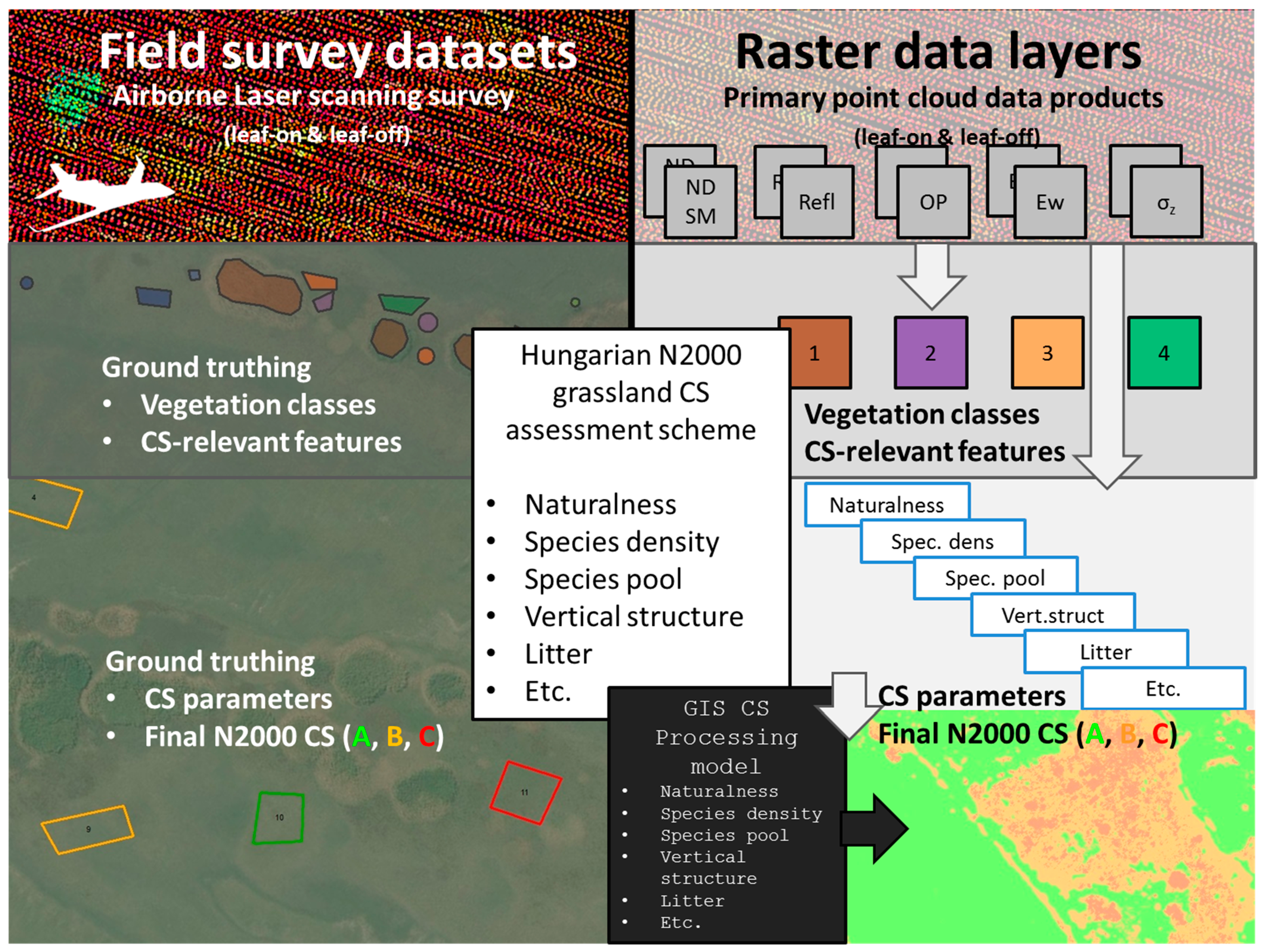
3. Methods
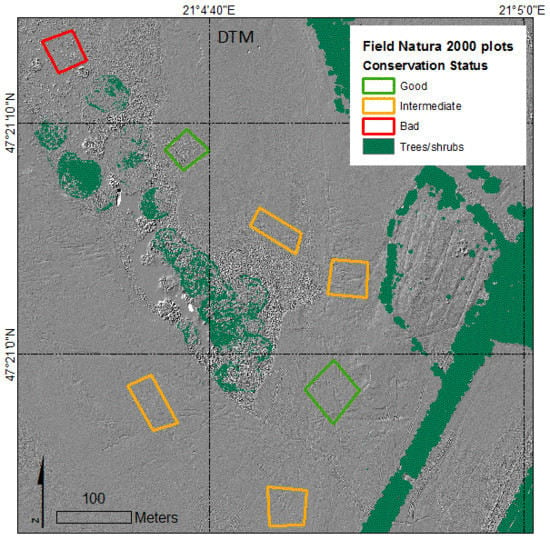
3.1. Study Site
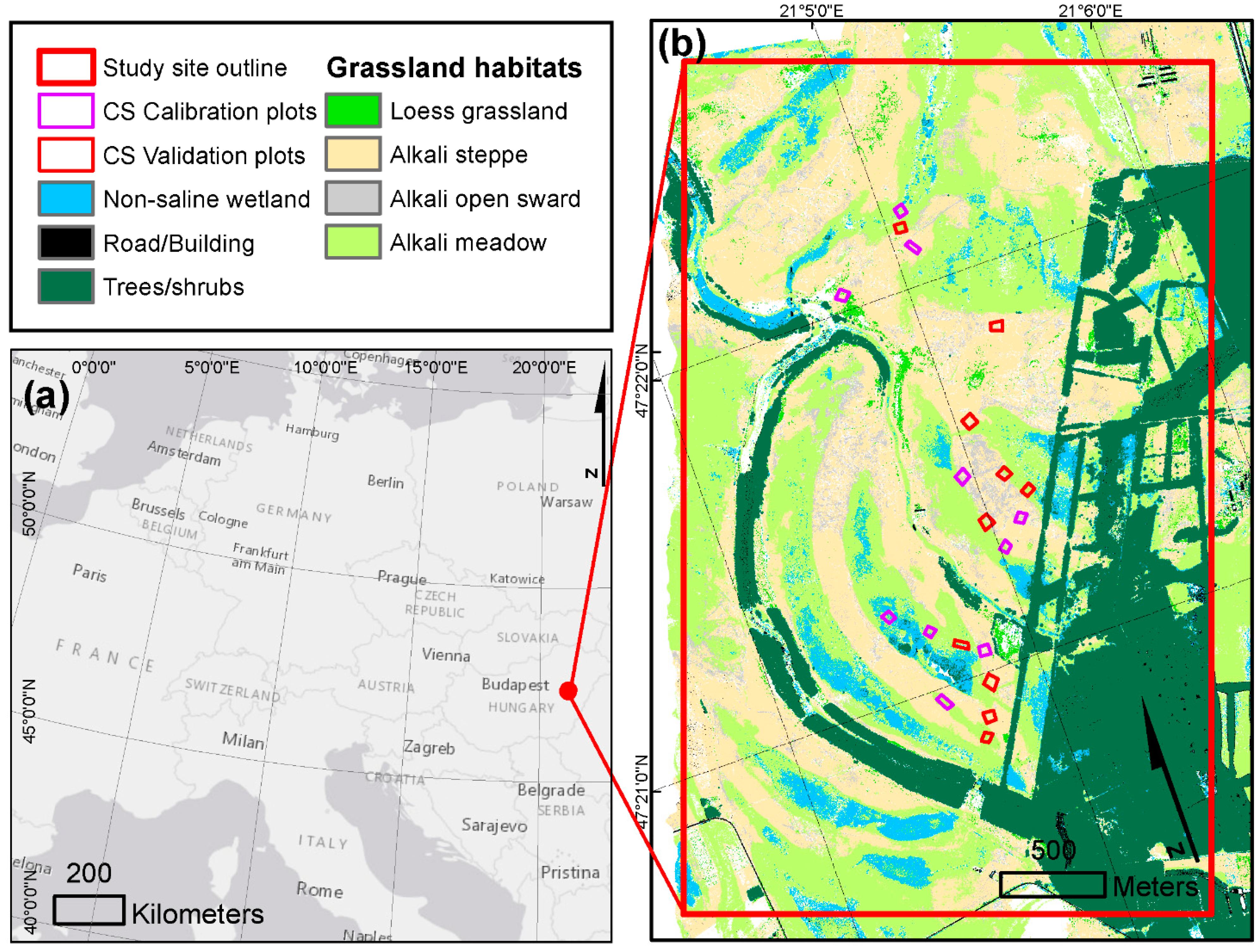
3.2. Field Data Collection
3.3. Calculation of the N2000 Assessment Scores
- Naturalness: this is defined based on the overall status, species pool, structure and management of a site. In Hungary, it is routinely used with a scale ranging from 5 (ecosystem in natural state) to 1 (a severely modified ecosystem). The assessment scheme assigns strong weighting to this parameter: a plot scores +10 points for naturalness values of 4 or 5, 0 points for naturalness of 3 and −5 points for naturalness of 1 or 2.
- Species density: According to the assessment scheme, “species density “is defined as the variation in the number of species within six 0.5 m × 0.5 m subplots. Alkali grasslands have a very fine mosaic structure and accordingly species density varies considerably even at the 0.5 m scale we investigated. If species density was found unfavorable, a score of −1 was assigned, otherwise 0.
- Inner patchiness is quantified based on the coverage, species composition, variability and respective area of patches of various vegetation within the assessment plot. This parameter is moderately weighted: +5 points are assigned to the plot if the patchiness corresponds to the typical patchiness of the habitat, −1 point is given if the patchiness is different (higher or lower).
- Vertical structure for grasslands is defined based on the presence and absence of typical “understory”, “medium level” or “top canopy” grasses and herbs. Weighting of the parameter is moderate: the score of +5 is assigned if the vertical structure corresponds to the typical composition of the habitat, −1 if it is different.
- Species pool is defined based on the most abundant species and the presence of species typical for Pannonic Salt Steppes and Salt Marshes. The assessment scheme adds strong emphasis to this parameter: +10 points are assigned if the species pool represents the habitat, −5 if the dominant species is not one of those typical for the habitat.
- Litter accumulation: This parameter is defined based on the amount of dry plant litter within the plot. Strong weighting is applied by the scheme since this is one of the most important potential problems in the studied habitat. +5 points are given if litter accumulation is not present, −1 point for a number of options including high litter cover, litter causing reduction in grass coverage or diversity or accumulation of weeds; finally, −10 points if litter facilitates the spread of invasive species. Here, the negative scores can add up if several negative criteria are fulfilled, so up to −13 points may be reached. In our study site, the grazing regime is the main driver of litter accumulation, with a delicate balance of avoiding both no litter but overgrazing and no overgrazing but eventual litter accumulation.
- Soil erosion is defined as an estimation of the intensity of ongoing erosion within the plot. The assessment scheme assigns moderate weighting to erosion, giving +5 points if there is no erosion or if it has a positive effect, or −1 for various negative effects. In alkali habitats, natural erosion maintains open alkali sward patches and thus generally has a positive effect in shaping the mosaic pattern of the vegetation.
- Shrub encroachment is quantified based on an estimate of the coverage of shrubs, their pattern and the list of shrub species observed. The presence of alien invasive shrub species receives a strong negative score (−10), closing of shrub canopy as a consequence of abandonment or disturbance [48] has low weighting (−1 point), and in case the distribution of shrubs is random and contributes to biodiversity [49], a moderate positive score of +5 is assigned.
- Weed encroachment is defined as the coverage of various weed species, categorized within the assessment scheme. For weed species with different growth strategies, different thresholds are assigned. This parameter is moderately weighed; the scheme assigns +5 points if weed cover is lower than 15% and −1 point if higher. Alkali habitats are less sensitive to weed encroachment as the harsh environment is intolerable for many common weed species.
- Disturbances are defined as the area ratio of anthropogenic features within the habitat that have a negative effect (incorrect grazing management, vehicle marks, paths, trampling, or rubbish). This parameter is strongly weighted by the scheme: If less than 10% of the plot is affected by any disturbance, +5 points are given, otherwise −1. In our case, the most important disturbances were improper grazing management and additionally treading by vehicles.
- Future threats are defined as any ongoing processes which might not have an influence at present but can be expected to have a negative effect on the habitat. This is a rather strongly weighted parameter, −5 points are assigned if a future threat is present, +5 if not. The most important future threat identified in the field is the ongoing lowering of the water table and subsequent drying of the site.
- Animal traces are also defined based on the area affected by animal presence, including grazing, burrowing, rooting, trampling and droppings. Moderate weighting is applied: if more than 50% of the plot is affected, it scores −5 points, otherwise +5. In our study site, which is managed by extensive grazing, the only negative effect observed for some patches was the already mentioned active overgrazing.
- Landscape context is defined based on the spatial context of the neighboring habitats: whether the habitat patch is neighbored by other natural habitats (local landscape context); whether the nearest similar habitat is within 100 m (wide area context), and finally whether there is a patch of invasive species in the vicinity. This parameter is weighed heavily: the favorable case scores +5, the threat of invasion −10 points. In case of our study site, protected alkali grasslands form a large continuous patch of 20 km2 only broken in some cases by forests, wetlands or roads.
3.4. Airborne Survey and Primary Data Products
- A Digital Terrain Model (DTM) was calculated from the leaf-off point cloud using the iterative robust interpolation algorithm [51] in SCOP++ [52]. Based on the DTM, normalized point heights were calculated both from the leaf-off and the leaf-on point cloud by subtracting the ground elevation, and separate output rasters of the interpolated normalized digital surface model (NDSM) and the mean and maximum normalized heights in each raster cell were produced.
- Surface texture, or roughness, is an important parameter describing the vertical distribution of points within a neighborhood, and is often closely related to vegetation canopy structure [53]. Therefore, rasters were also generated from roughness indices calculated on the normalized point cloud: σz, σ0, and variance.
- Echo amplitude was calibrated to reflectance, using field spectroscopy measurements of homogeneous targets (asphalt and concrete surfaces) [54]. The mean reflectance of the points within each 0.5 m cell and the variance of the point reflectances with two different kernel sizes (3 × 3 and 5 × 5 pixels) were written to separate output rasters.
- Echo width is a measure of vegetation canopy structure [25,55], and was calculated separately by online waveform processing for each point by the sensor itself [56]. Mean echo width, maximum echo width from the first echoes and variance of echo width with two different kernel sizes were calculated for each raster.
- Finally, as a measure of terrain texture, openness rasters (minimum, maximum, average and difference between the minimum and maximum openness) of the DTM [57] were calculated, in order to enhance linear features, sharp edges and local minima and maxima in the terrain.

3.5. Classification of Vegetation and CS-Relevant Features
3.6. Selection and Calibration of CS Parameters
3.7. Calculation and Validation of Final CS Scores
4. Results
4.1. Main Classification Products and Accuracies
- Land Cover: first of all, the area of the habitat in focus, Pannonic Salt Steppes and Salt Marshes (1530) had to be determined and separated from all other land cover types, which were trees and shrubs, artificial surfaces and non-alkali wetlands. For these categories, producers’ and users’ accuracies based on more than 10,000 validation pixels for each class were typically around 90% (Supplementary Table S3), and Kappa was 0.83, indicating very strong agreement. Non-alkali wetlands proved to be a rather problematic category, on one hand due to the smooth transition towards alkali tall grass wetlands, on the other hand to shrubs with similar height, but even this class had accuracy measures above 65%.
- Main vegetation categories/alkali subhabitats (Supplementary Table S4): For this scenario, the goal was to separate the three most important vegetation categories of the 1530 habitat type: alkali steppes, open alkali swards and alkali meadows [2]. Loess grasslands, Carex and Juncus dominated wet patches and non-alkali wetlands were added as outgroups together with the category “vegetation background”. The Cohen’s Kappa of 0.625 shows a good agreement between the ALS-derived pixel-level classification and the ground truth training data. Within 1530, dry grassland and wetland categories are rarely confused by the classifier. The main sources of error are discrimination between short grass steppes and open alkali swards, and between tall Carex stands and alkali meadows.
- Alkali vegetation associations: This was the finest classification level, aiming at identifying each of the alkali grassland and wetland associations. The probabilities assigned to the various associations for each pixel by the random forest classifier were further processed as CS variables. For this set of 16 classes, total accuracy is 62.9%, with a Kappa of 0.579. Most of the misclassifications happened within the main vegetation categories (alkali steppe, alkali sward, alkali meadow and non-alkali wetland) as demonstrated by the error report (Supplementary Table S5).
- Anthropogenic features and disturbance: The main targets of this scenario were the probability of weed growth and damage by vehicle tracks, each represented by a single-category probability raster during further processing. Weeds had an F1 score of 69%, and rather low quantitative deviation but higher allocation deviation [64]. Unpaved roads were overestimated, with quantitative deviation also high and user’s accuracy of only 48%. Nevertheless, the Kappa of this scenario is 0.77, indicating a strong agreement (Supplementary Table S6).
- Trees and shrubs: In this scenario, we aimed to identify trees and shrubs and separate alien and native species among them. Accuracies were around 80%, non-native species were slightly overestimated (Supplementary Table S7), Cohen’s Kappa was 0.79. The classified hard boundary raster was used for further processing.
4.2. ALS Products Identified for CS Parameters and CS Scoring
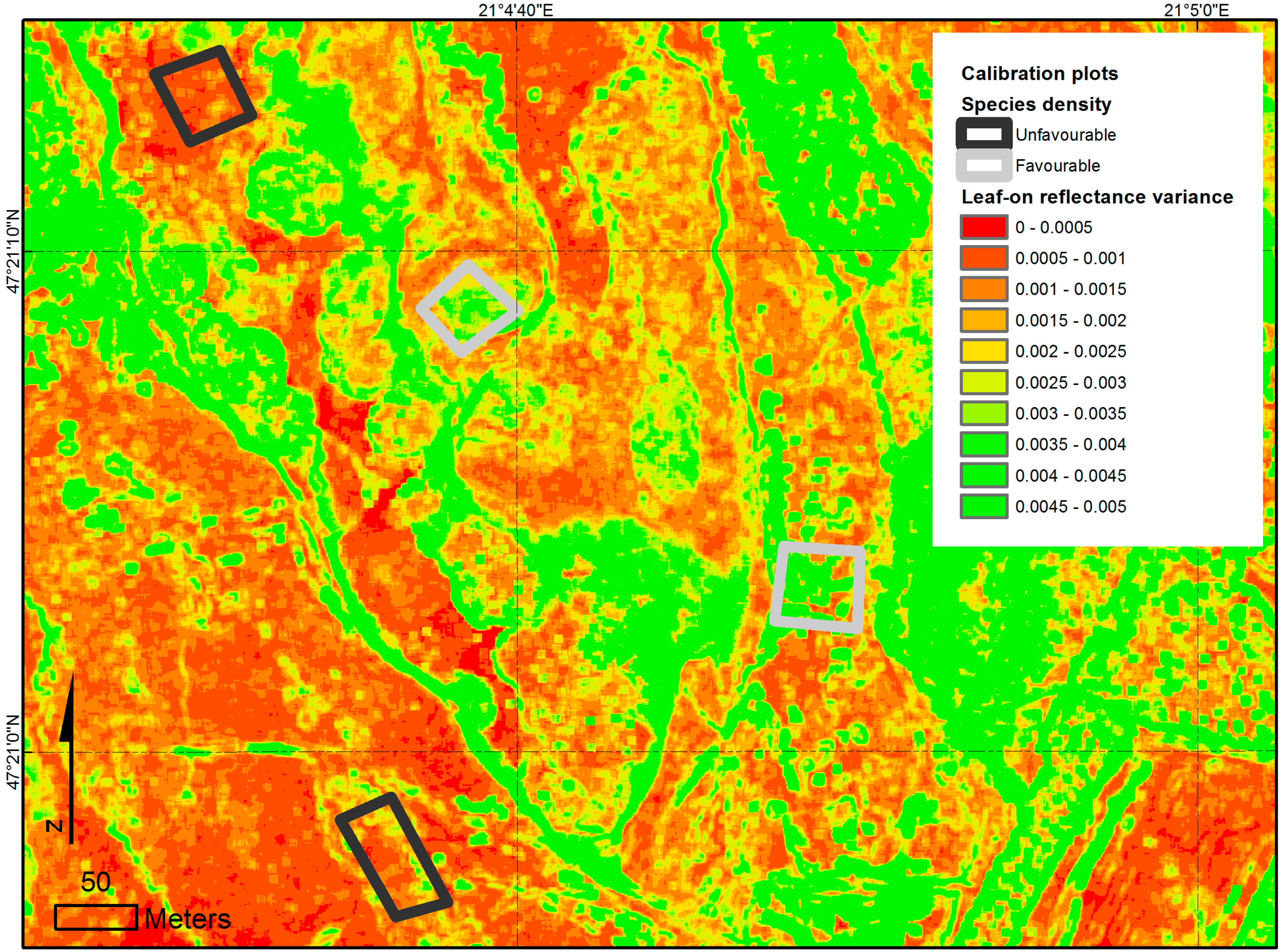
- Naturalness: we used the difference between the leaf-on and leaf-off reflectance. In case of the study site, we observed in the field that the most important factor governing the naturalness of a habitat was the grazing regime: over- or undergrazed patches were in a worse naturalness state than moderately grazed areas. At the 1550 nm wavelength of the ALS sensor, reflectivity of vegetation is proportional to the water content of the cells and thus to the wet or dry biomass [29]. Therefore, if the difference was below 0.2 in meadows or 0.05 in short-grass habitats, this was understood to mean that the amount of standing biomass during the summer grazing season was not much higher or even lower than during the leaf-off season when the grass is typically grazed to the ground. A total of 78.8% of the pixels within the CS validation plots had the correct score based on this calculation. Eight of the plots had high naturalness and more than 80% of their pixels were correctly labeled (Figure 4). Two plots had low naturalness, one of these was incorrectly detected, the majority of the other plot was correct.
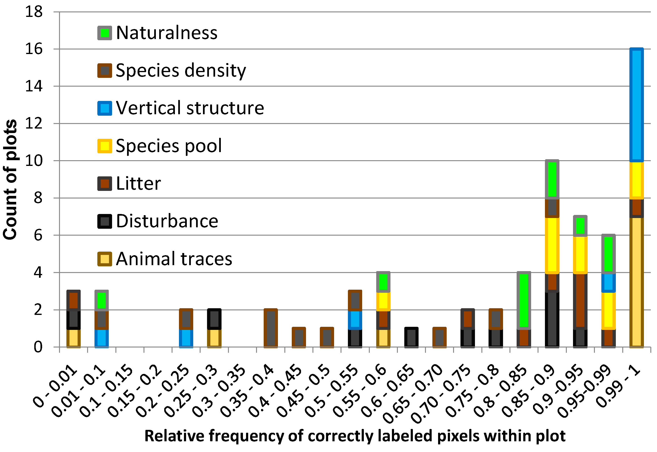
- Based on the Spectral Variation Hypothesis [67], species density was represented with the variance of the leaf-on point reflectance within a pixel. To follow the different characteristic scales for long and short grass habitats, a 5 × 5 cell kernel was applied for meadows and a 3 × 3 cell kernel for steppe and sward, but the threshold separating favorable and unfavorable species density was 0.001 in each case. 47.2% of all the pixels in the CS validation plots had the correct score, with only a single plot being more than 80% correct and half of the validation plots having more incorrect species density scores than correct ones. Two plots had unfavorable species density; the majority of the pixels in one of them was correctly identified.
- Inner patchiness: All plots showed constant favorable patchiness; therefore, we assigned the same score to all alkali habitats (based on the grassland habitat mask). Based on the land cover scenario, this mask has accuracies above 90% (Supplementary Table S3).
- Vertical structure: The difference between leaf-on and leaf-off maximum normalized point height was identified as a proxy for vertical structure. We applied a threshold of −0.15 m separating favorable and unfavorable conditions. A total of 82% of the investigated pixels were correctly classified, six plots were over 99% correct, but two (including the single one with unfavorable vertical structure) had less than 50% correct pixels.
- Species pool: We used the summed probability of alkali grassland associations (from the association-level scenario output) as a proxy for this variable. These values were summed separately for the associations corresponding to meadows and short grasslands/open swards, with unfavorable species pool assigned to a pixel if the probability of it belonging to any of these was below 50% and favorable if above this limit. Only one calibration CS plot and no validation plots had unfavorable species pool, which explains the observed performance of this ALS-based indicator: 91% of all validation pixels were labeled correctly, with no misclassified plots.
- Litter accumulation: The difference in leaf-on and leaf-off reflectance proved to correspond to the pattern in the litter accumulation of our calibration plots (threshold >0.3 unfavorable). The various levels of negative effects of litter could not be resolved from our sensor data. We assigned either +5 or −1 point to a pixel based on litter accumulation, and classified only the quantity of litter but not its effect (see Section 3.3) Four validation plots had favorable litter quantity and six unfavorable, and all but one (unfavorable) were correctly detected with 79% of all the validation pixels well identified.
- Soil erosion: All field plots received favorable scores for this factor, since only positive effects of erosion were observed in the site. Therefore, we simply assigned the favorable value to all pixels belonging to the alkali grassland habitats. The accuracy of this indicator is the same as the accuracy of grassland masking.
- Shrubs: None of our field plots contained any shrubs, but both native and alien invasive shrubs were present in the site. Following the assessment scheme, we used the scenario “trees and shrubs” with a morphological opening operation [68] to identify dense stands. This was compared with the class “alien invasive trees/shrubs” to identify separately the “low density”, the “dense native” and the “dense alien invasive” classes. Since this indicator directly relies on the output of the tree/shrub classification layers, its accuracy is at or above 65% (Supplementary Table S7).
- Weeds: We used the single-band weed probability layer from the “anthropogenic features and disturbances” scenario. The threshold for unfavorable presence of weeds was assigned to be 65% probability in absence of more detailed calibration data. Again, the reliability of this indicator could not be tested; the accuracy of the weed probability layer is quantified within the respective classification scenario (Supplementary Table S6).
- Disturbances: For grazing regime, difference in maximum normalized height was used again for meadows, with differences below −0.15 representing overgrazing and above −0.02 representing undergrazing and litter accumulation. In short grasslands, overgrazing is less of an issue as the standing crop is low anyway. Again, we used the difference in leaf-on and leaf-off reflectance and the already established threshold of <0.3 for undergrazing. As for treading by vehicles, we took the probability of the class “unpaved road” from the “anthropogenic features and disturbances” scenario, which included established field roads and also individual vehicle tracks, and set a threshold of 65% probability to identify any pixel where tracks can be suspected. Six of our CS validation plots received a negative score for disturbance while four were in favorable state; all except one (unfavorable) were correctly identified. A total of 64% of the pixels within the total area of the validation plots was labeled correctly, and four plots had more than 85% correctly labeled pixels (two in favorable and two in unfavorable status). According to the assessment scheme, a plot already qualifies as disturbed if 10% of its area is affected, which explains some of the plots with lower proportions labeled correctly, but not the single case of a disturbed plot where less than 1% of the pixels were correct.
- Future threats: The gradual lowering of the water table as the most important future threat has a long-term dimension in time and therefore cannot be identified by two remote sensing surveys within a few months. However, it correlates closely with terrain elevation: lower lying areas are less threatened. The DTM was used as a source dataset and since all the calibration/validation polygons were estimated in the field to be affected by this risk, only the areas lying below the lowest calibration plot (127.25 m) were considered to be unaffected, which are nearly all non-alkali wetlands in our site. The accuracy of this parameter could not be tested either, but since the accuracy of the DTM is within 5 cm, the area of the study area within ±2.5 cm of this threshold was calculated, which is 5% of the total area. No part of the CS calibration or validation plots lies in this elevation interval.
- Animal traces: active presence and overgrazing of livestock was calculated from the difference in leaf-on and leaf-off maximum normalized height, but assigned a slightly different threshold of −0.17 compared to the threshold for litter accumulation in accordance with the scheme. One of the CS validation plots was in an unfavorable status in terms of animal traces, this plot had no correctly labeled pixels, and two other plots also had less than 60% correct pixels. Therefore, the overall ratio of 82% correctly labeled pixels within the CS validation plots is an overestimation of performance.
- Landscape context: The CS scheme defines two levels of landscape context. Therefore, we counted for each pixel the amount of alkali grassland pixels in its neighborhood with two different kernels: 15 × 15 pixels representing the neighboring environment (with a threshold of 220 pixels representing a large number of similar neighbors) and 100 × 100 pixels to imitate the rule of “closest similar habitat is not more than 100 m away”. The accuracy of these indicators corresponds to the accuracy of the alkali habitat masking in the land cover scenario, which is 95% (Supplementary Table S3).

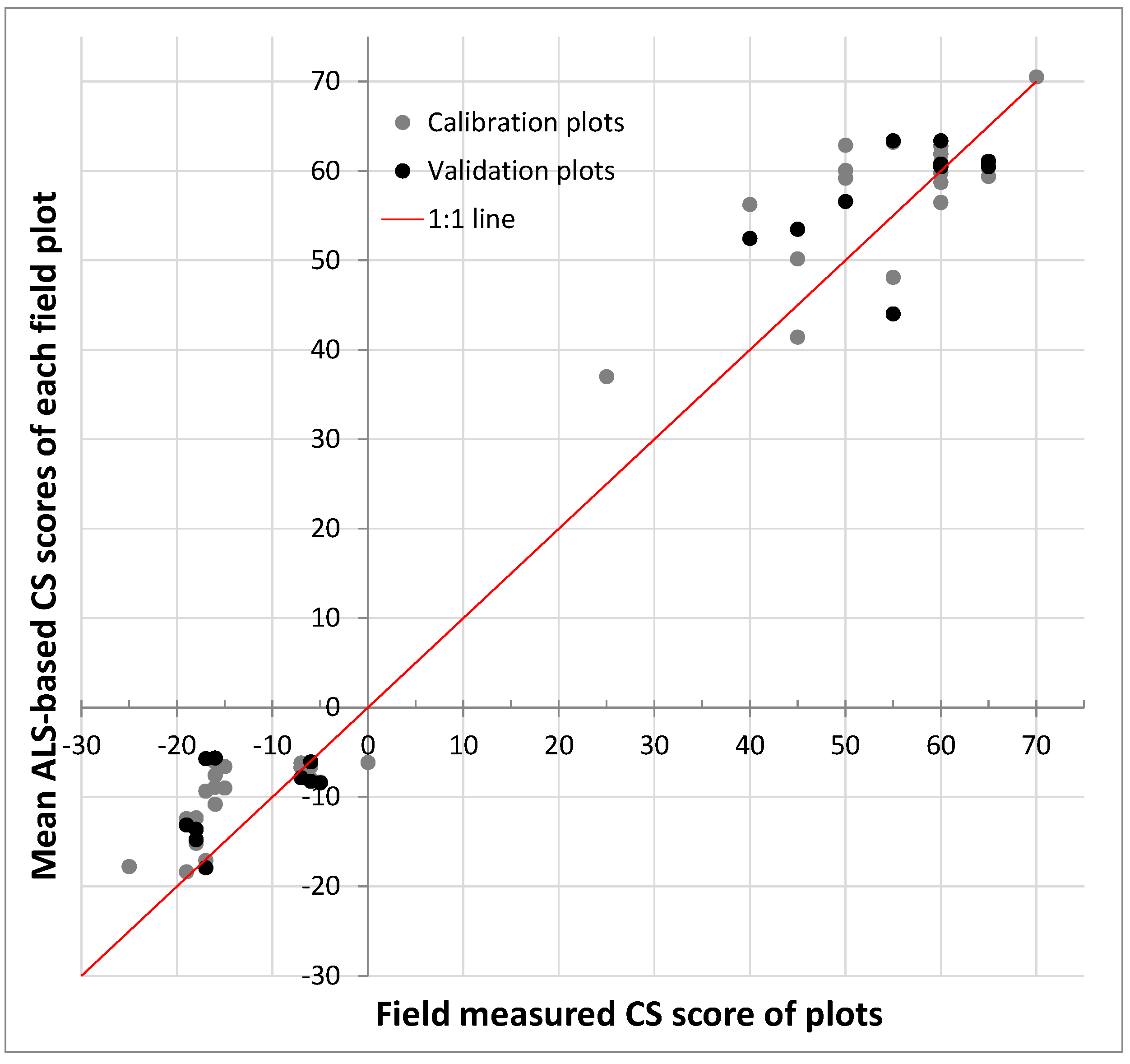
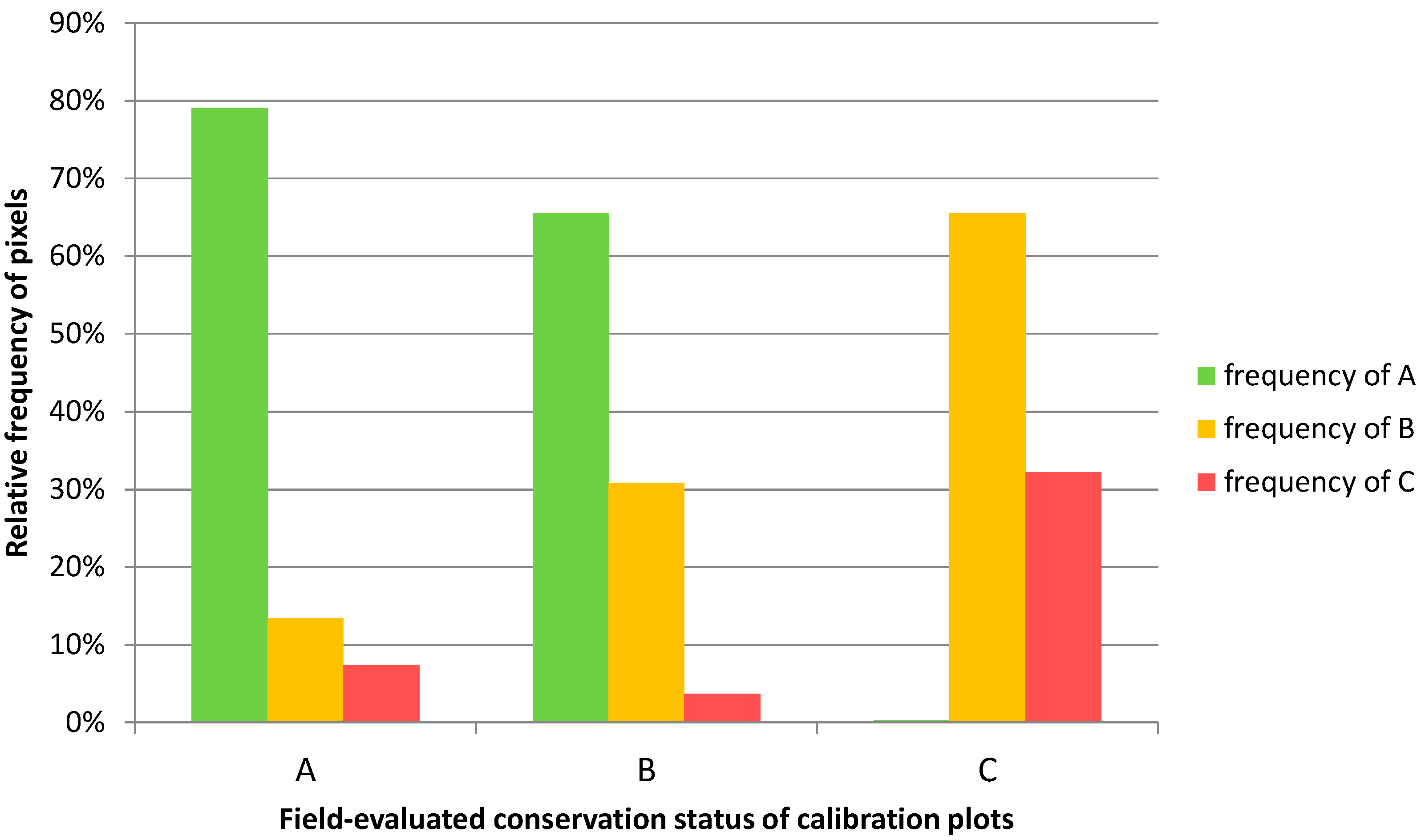
4.3. Final CS Modeling Algorithm and its Performance

- If a plot has more than 70% pixels in class A the plot qualifies as A.
- If A is below 10% and C is above 25% then the plot belongs to C.
- In all other cases the plot qualifies as B.

5. Discussion
5.1. Reference Data Availability
5.2. ALS Data and its Effectiveness for Quantifying All CS Relevant Parameters for N2000: Errors, Uncertainties, Accuracies
5.3. Mapping Natura 2000 Conservation Status: Errors, Uncertainties, Accuracies
5.4. The HQ/CS Model Directly Based on the Hungarian N2000 Grassland Evaluation Scheme
5.5. Method for ALS-Assisted N2000 CS Mapping of Alkali Grasslands
5.6. Data Products of the Assessment and Their Use in Conservation
5.7. Outlook
6. Conclusions
Supplementary Materials
Acknowledgments
Author Contributions
Conflicts of Interest
References
- European Commission DG Environment. In Interpretation Manual of European Union Habitats; EUR 28; Nature and Biodiversity: Bruxelles, Belgium, 2013; p. 146.
- Deák, B.; Valkó, O.; Alexander, C.; Mücke, W.; Kania, A.; Tamás, J.; Heilmeier, H. Fine-scale vertical position as an indicator of vegetation in alkali grasslands—Case study based on remotely sensed data. Flora 2014, 209, 693–697. [Google Scholar] [CrossRef]
- Valkó, O.; Tóthmérész, B.; Kelemen, A.; Simon, E.; Miglécz, T.; Lukács, B.; Török, P. Environmental factors driving vegetation and seed bank diversity in alkali grasslands. Agric. Ecosyst. Environ. 2014, 182, 80–87. [Google Scholar] [CrossRef]
- Deák, B.; Valkó, O.; Tóthmérész, B.; Török, P. Alkali marshes of Central Europe—Ecology, management and nature conservation. In Salt Marshes—Ecosystem, Vegetation and Restoration Strategies; Shao, H.-B., Ed.; Nova Science Publishers: New York, NY, USA, 2014; pp. 1–11. [Google Scholar]
- Kelemen, A.; Török, P.; Valkó, O.; Miglécz, T.; Tóthmérész, B. Mechanisms shaping plant biomass and species richness: Plant strategies and litter effect in alkali and loess grasslands. J. Veg. Sci. 2013, 24, 1195–1203. [Google Scholar] [CrossRef]
- Deák, B.; Valkó, O.; Török, P.; Tóthmérész, B. Solonetz meadow vegetation (Beckmannion eruciformis) in East-Hungary–an alliance driven by moisture and salinity. TUEXENIA 2014, 34, 187–203. [Google Scholar]
- European Commission. Council Directive 92/43/EEC of 21 May 1992 on the conservation of natural habitats and of wild fauna and flora. Official Journal of the European Union 1992, 206, 7–50. [Google Scholar]
- Weber, N.; Christophersen, T. The influence of non-governmental organisations on the creation of Natura 2000 during the European Policy process. For. Policy Econ. 2002, 4, 1–12. [Google Scholar] [CrossRef]
- European Topic Centre on Biological Diversity. In Habitats Directive Article 17 Report (2001–2006) Data Completeness, Quality and Coherence; ETBD: Paris, France, 2008; p. 24.
- European Commission. The EU Biodiversity Strategy to 2020; DG Environment, Publications Office of the European Union: Luxembourg, Luxembourg, 2011; p. 28. [Google Scholar]
- Vanden Borre, J.; Paelinckx, D.; Mücher, C.A.; Kooistra, L.; Haest, B.; de Blust, G.; Schmidt, A.M. Integrating remote sensing in Natura 2000 habitat monitoring: Prospects on the way forward. J. Nat. Conserv. 2000, 19, 116–125. [Google Scholar]
- Simonson, W.D.; Allen, H.D.; Coomes, D.A. Applications of airborne LiDAR for the assessment of animal species diversity. Methods Ecol. Evol. 2014, 5, 719–729. [Google Scholar] [CrossRef]
- Asner, G.P.; Hughes, F.R.; Mascaro, J.; Uowoli, A.L.; Knapp, D.E.; Jacobson, J.; Kennedy-Bowdoin, T.; Clark, J.K. High-resolution carbon mapping on the million-hectare Island of Hawaii. Front. Ecol. Environ. 2011, 9, 434–439. [Google Scholar] [CrossRef]
- Corbane, C.; Lang, S.; Pipkins, K.; Alleaume, S.; Deshayes, M.; Millán, V.E.G.; Strasser, T.; Borre, J.V.; Toon, S.; Michael, F. Remote sensing for mapping natural habitats and their conservation status—New opportunities and challenges. Int. J. Appl. Earth Obs. Geoinf. 2014, 37, 7–16. [Google Scholar] [CrossRef]
- White, R.P.; Murray, S.; Rohweder, M. Pilot Analysis of Global Ecosystems—Grassland Ecosystems; World Resources Institute: Washington, DC, USA, 2000; p. 81. [Google Scholar]
- Veen, P.; Jefferson, R.; de Smidt, J.; van der Straaten, J. Grasslands in Europe of High Nature Value; KNNV Publishing: Zeist, The Netherlands, 2009; p. 320. [Google Scholar]
- Burai, P.; Deák, B.; Valkó, O.; Tomor, T. Classification of herbaceous vegetation using airborne hyperspectral imagery. Remote Sens. 2015, 7, 2046–2066. [Google Scholar] [CrossRef]
- Schuster, C.; Schmidt, T.; Conrad, C.; Kleinschmit, B.; Förster, M. Grassland habitat mapping by intra-annual time series analysis—Comparison of RapidEye and TerraSAR-X satellite data. Int. J. Appl. Earth Obs. Geoinf. 2015, 34, 25–34. [Google Scholar] [CrossRef]
- Buck, O.; Millán, V.E.G.; Klink, A.; Pakzad, K. Using information layers for mapping grassland habitat distribution at local to regional scales. Int. J. Appl. Earth Obs. Geoinf. 2015, 37, 83–89. [Google Scholar] [CrossRef]
- Reese, H.; Nyström, M.; Nordkvist, K.; Olsson, H. Combining airborne laser scanning data and optical satellite data for classification of alpine vegetation. Int. J. Appl. Earth Obs. Geoinf. 2014, 27, 81–90. [Google Scholar] [CrossRef]
- Bork, E.W.; Su, J.G. Integrating LiDAR data and multispectral imagery for enhanced classification of rangeland vegetation: A meta analysis. Remote Sens. Environ. 2007, 111, 11–24. [Google Scholar] [CrossRef]
- Ichter, J.; Evans, D.; Richard, D. Terrestrial Habitat Mapping in Europe: An Overview; TH-AK-14-001-EN-N; European Environmental Agency: Luxembourg, 2014; p. 152. [Google Scholar]
- Corbane, C.; Deshayes, M.; Elena, G.M.V.; Strasser, T.; Vanden Borre, J.; Spanhove, T.; Förster, M.; Lang, S.; Pernkopf, L. Deliverable 3.2, Technical Synthesis on the Possibilities and Limits of RS for Mapping Natural Habitats; Institut National de Recherce en Sciences et Technologies pour l’Environement et l’Agriculture: Montpellier, France, 2013; p. 82. [Google Scholar]
- Ward, R.D.; Burnside, N.G.; Joyce, C.B.; Sepp, K. The use of medium point density LiDAR elevation data to determine plant community types in Baltic coastal wetlands. Ecol. Indic. 2013, 33, 96–104. [Google Scholar] [CrossRef]
- Zlinszky, A.; Schroiff, A.; Kania, A.; Deák, B.; Mücke, W.; Vári, Á.; Székely, B.; Pfeifer, N. Categorizing grassland vegetation with full-waveform airborne laser scanning: A feasibility study for detecting Natura 2000 Habitat Types. Remote Sens. 2014, 6, 8056–8087. [Google Scholar] [CrossRef]
- Feilhauer, H.; Thonfeld, F.; Faude, U.; He, K.S.; Rocchini, D.; Schmidtlein, S. Assessing floristic composition with multispectral sensors—A comparison based on monotemporal and multiseasonal field spectra. Int. J. Appl. Earth Obs. Geoinf. 2013, 21, 218–229. [Google Scholar] [CrossRef]
- Mücher, C.A.; Kooistra, L.; Vermeulen, M.; Borre, J.V.; Haest, B.; Haveman, R. Quantifying structure of Natura 2000 heathland habitats using spectral mixture analysis and segmentation techniques on hyperspectral imagery. Ecol. Indic. 2013, 33, 71–81. [Google Scholar] [CrossRef]
- Fava, F.; Parolo, G.; Colombo, R.; Gusmeroli, F.; Della Marianna, G.; Monteiro, A.T.; Bocchi, S. Fine-scale assessment of hay meadow productivity and plant diversity in the European Alps using field spectrometric data. Agric. Ecosyst. Environ. 2010, 137, 151–157. [Google Scholar] [CrossRef]
- Sims, D.A.; Gamon, J.A. Estimation of vegetation water content and photosynthetic tissue area from spectral reflectance: A comparison of indices based on liquid water and chlorophyll absorption features. Remote Sens. Environ. 2003, 84, 526–537. [Google Scholar] [CrossRef]
- Stratoulias, D.; Balzter, H.; Zlinszky, A.; Tóth, V.R. Assessment of ecophysiology of lake shore reed vegetation based on chlorophyll fluorescence, field spectroscopy and hyperspectral airborne imagery. Remote Sens. Environ. 2015, 157, 72–84. [Google Scholar] [CrossRef] [Green Version]
- Psomas, A. Hyperspectral Remote Sensing for Ecological Analyses of Grassland Ecosystems—Spectral Separability and Derivation of NPP Related Biophysical and Biochemical Parameters. Ph.D. Thesis, Universität Zürich, Zürich, Switzerland, 2008. [Google Scholar]
- Oldeland, J.; Wesuls, D.; Rocchini, D.; Schmidt, M.; Jürgens, N. Does using species abundance data improve estimates of species diversity from remotely sensed spectral heterogeneity? Ecol. Indic. 2010, 10, 390–396. [Google Scholar] [CrossRef]
- Franke, J.; Keuck, V.; Siegert, F. Assessment of grassland use intensity by remote sensing to support conservation schemes. J. Nat. Conserv. 2012, 20, 125–134. [Google Scholar] [CrossRef]
- Schuster, C.; Ali, I.; Lohmann, P.; Frick, A.; Foerster, M.; Kleinschmit, B. Towards detecting swath events in TerraSAR-X time series to establish NATURA 2000 grassland habitat swath management as monitoring parameter. Remote Sens. 2011, 3, 1308–1322. [Google Scholar] [CrossRef]
- Neumann, C. Synthese von Ökologischer Gradientenanalyse und Hyperspektraler Fernerkundung zum Monitoring Naturschutzfachlich Bedeutsamer Offenlandschaften. Master’s Thesis, Universität Potsdam, Potsdam, Germany, 2010. [Google Scholar]
- Foody, G. Fuzzy modelling of vegetation from remotely sensed imagery. Ecol. Model. 1996, 85, 3–12. [Google Scholar] [CrossRef]
- Spanhove, T.; Vanden Borre, J.; Delalieux, S.; Haest, B.; Paelinckx, D. Can remote sensing estimate fine-scale quality indicators of natural habitats? Ecol. Indic. 2012, 18, 403–412. [Google Scholar] [CrossRef]
- Müller, J.; Brandl, R. Assessing biodiversity by remote sensing in mountainous terrain: The potential of LiDAR to predict forest beetle assemblages. J. Appl. Ecol. 2009, 46, 897–905. [Google Scholar] [CrossRef]
- Lindberg, E.; Roberge, J.-M.; Johansson, T.; Hjältén, J. Can airborne laser scanning or satellite images, or a combination of the two, be used to predict the abundance and species richness of birds and beetles at a patch scale? In Proceedings of the International Workshop on Remote Sensing and GIS for Monitoring of Habitat Quality, Vienna, Austria, 24–25 September 2014; Pfeifer, N., Zlinszky, A., Eds.; Department of Geodesy and Geoinformation, Vienna University of Technology: Vienna, Austria, 2014; pp. 138–143. [Google Scholar]
- Palminteri, S.; Powell, G.V.N.; Asner, G.P.; Peres, C.A. LiDAR measurements of canopy structure predict spatial distribution of a tropical mature forest primate. Remote Sens. Environ. 2012, 127, 98–105. [Google Scholar] [CrossRef]
- Simonson, W.D.; Allen, H.D.; Coomes, D.A. Remotely sensed indicators of forest conservation status: Case study from a Natura 2000 site in southern Portugal. Ecol. Indic. 2013, 24, 636–647. [Google Scholar] [CrossRef]
- Delalieux, S.; Somers, B.; Haest, B.; Spanhove, T.; Vanden Borre, J.; Mücher, C.A. Heathland conservation status mapping through integration of hyperspectral mixture analysis and decision tree classifiers. Remote Sens. Environ. 2012, 126, 222–231. [Google Scholar] [CrossRef]
- Frick, A. Entwicklung eines Wissensbasierten Klassifikationsverfahrens und Anwendung in Brandenburg. Ph.D. thesis, Technische Universität Berlin, Berlin, Germany, 2006. [Google Scholar]
- Riedler, B.; Pernkopf, L.; Strasser, T.; Lang, S.; Smith, G. A composite indicator for assessing habitat quality of riparian forests derived from earth observation data. Int. J. Appl. Earth Obs. Geoinf. 2014, 37, 114–123. [Google Scholar] [CrossRef]
- Török, P.; Kapocsi, I.; Deák, B. Conservation and management of alkali grassland biodiversity in Central Europe. In Grasslands: Types, Biodiversity and Impacts; Zhang, W.J., Ed.; Nova Science Publishers Inc.: New York, NY, USA, 2012; pp. 109–118. [Google Scholar]
- Molnár, Z.; Máté, A. 1530 Pannon szikes styeppek és mocsarak. In Natura 2000 Fajok és Élőhelyek Magyarországon; Haraszthy, L., Ed.; Pro Vértes Közalapítvány: Csákvár, Hungary, 2014; pp. 761–766. [Google Scholar]
- Valbuena, R. Integrating airborne laser scanning with data from global navigation satellite systems and optical sensors. In Forestry Applications of Airborne Laser Scanning; Springer: Dordrecht, The Netherlands, 2014; pp. 63–88. [Google Scholar]
- Poschlod, P.; Bakker, J.P.; Kahmen, S. Changing land use and its impact on biodiversity. Basic Appl. Ecol. 2005, 6, 93–98. [Google Scholar] [CrossRef]
- Kasari, L.; Gazol, A.; Kalwij, J.M.; Helm, A. Low shrub cover in alvar grasslands increases small-scale diversity by promoting the occurrence of generalist species. Tuexenia 2013, 33, 293–308. [Google Scholar]
- Pfeifer, N.; Mandlburger, G.; Otepka, J.; Karel, W. OPALS—A framework for Airborne Laser Scanning data analysis. Comput. Environ. Urban Syst. 2014, 45, 125–136. [Google Scholar] [CrossRef]
- Kraus, K.; Pfeifer, N. Determination of terrain models in wooded areas with airborne laser scanner data. ISPRS J. Photogramm. Remote Sens. 1998, 53, 193–203. [Google Scholar] [CrossRef]
- Pfeifer, N.; Stadler, P.; Briese, C. Derivation of Digital Terrain Models in the SCOP++ environment. In OEEPE Workshop on Airborne Laser Scanning and Interferometric SAR for Detailed Digital Elevation Models; Bundesamt für Kartographie und Geodäsie: Frankfurt, Germany, 2001; p. 13. [Google Scholar]
- Zlinszky, A.; Mücke, W.; Lehner, H.; Briese, C.; Pfeifer, N. Categorizing wetland vegetation by airborne laser scanning on Lake Balaton and Kis-Balaton, Hungary. Remote Sens. 2012, 4, 1617–1650. [Google Scholar] [CrossRef]
- Lehner, H.; Briese, C. Radiometric calibration of full-waveform airborne laser scanning data based on natural surfaces. Int. Arch. Photogramm. Remote Sens. Spat. Inf. Sci. 2010, 38, 360–365. [Google Scholar]
- Wagner, W.; Hollaus, M.; Briese, C.; Ducic, V. 3D vegetation mapping using small-footprint full-waveform airborne laser scanners. Int. J. Remote Sens. 2008, 29, 1433–1452. [Google Scholar] [CrossRef]
- Pfennigbauer, M.; Ullrich, A. Improving Quality of Laser Scanning Data Acquisition through Calibrated Amplitude and Pulse Deviation Measurement; Laser Radar Technology and Applications XV, Orlando, FL, USA, 2010; Turner, M.D., Kamerman, G.H., Eds.; SPIE: Orlando, FL, USA, 2010; p. 76841F. [Google Scholar]
- Doneus, M. Openness as visualization technique for interpretative mapping of airborne LiDAR derived topographic models. Remote Sens. 2013, 5, 6427–6442. [Google Scholar] [CrossRef]
- Bastin, L.; Fisher, P.F.; Wood, J. Visualizing uncertainty in multi-spectral remotely sensed imagery. Comput. Geosci. 2002, 28, 337–350. [Google Scholar] [CrossRef]
- Kania, A.; Zlinszky, A. Vegetation Classification Studio: A software tool for remote sensing based vegetation classification. Unpublished work. 2015. [Google Scholar]
- Kania, A.; Zlinszky, A. Gimme My Vegetation Map in an Hour! Towards Operational Vegetation Classification and Mapping: An Automated Software Workflow. In Proceedings of the International Workshop on Remote Sensing and GIS for Monitoring of Habitat Quality, Vienna, Austria, 24–25 September 2014; Pfeifer, N., Zlinszky, A., Eds.; Department of Geodesy and Geoinformation, Vienna University of Technology: Vienna, Austria, 2014; pp. 52–55. [Google Scholar]
- Zlinszky, A.; Deák, B.; Kania, A.; Schroiff, A.; Pfeifer, N. Natura 2000 Habitat Quality Mapping in a Pannonic Salt Steppe from Full-Waveform Airborne Laser Scanning. In Proceedings of the International Workshop on Remote Sensing and GIS for Monitoring of Habitat Quality, Vienna, Austria, 24–25 September 2014; Pfeifer, N., Zlinszky, A., Eds.; Department of Geodesy and Geoinformation, Vienna University of Technology: Vienna, Austria, 2014; pp. 130–134. [Google Scholar]
- Breiman, L. Random forests. Mach. Learn. 2001, 45, 5–32. [Google Scholar] [CrossRef]
- Congalton, R.G. A review of assessing the accuracy of classifications of remotely sensed data. Remote sens. Environ. 1991, 37, 35–46. [Google Scholar] [CrossRef]
- Pontius, R.G., Jr.; Millones, M. Death to Kappa: Birth of quantity disagreement and allocation disagreement for accuracy assessment. Int. J. Remote Sens. 2011, 32, 4407–4429. [Google Scholar] [CrossRef]
- Borhidi, A.; Kevey, B.; Lendvai, G. Plant Communities of Hungary; Akadémiai Kiadó: Budapest, Hungary, 2012; p. 544. [Google Scholar]
- Zlinszky, A.; Timár, G.; Weber, R.; Székely, B.; Briese, C.; Ressl, C.; Pfeifer, N. Observation of a local gravity potential isosurface by airborne LiDAR of Lake Balaton, Hungary. Solid Earth 2014, 5, 355–369. [Google Scholar] [CrossRef] [Green Version]
- Palmer, M.W.; Earls, P.G.; Hoagland, B.W.; White, P.S.; Wohlgemuth, T. Quantitative tools for perfecting species lists. Environmetrics 2002, 13, 121–137. [Google Scholar] [CrossRef]
- Hollaus, M.; Wagner, W.; Molnar, G.; Mandlburger, G.; Nothegger, C.; Otepka, J. Delineation of Vegetation and Building Polygons from Full-Waveform Airborne LiDAR Data Using OPALS Software. In Proceedings of the Geospatial Data and Geovisualization: Environment, Security, and Society, Special Joint Symposium of ISPRS Technical Commission IV and AutoCarto 2010 in Conjunction with ASPRS/GaGIS Speciality Conference, Orlando, FL, USA, 15–19 November 2010; ISPRS: Orlando, FL, USA, 2010; p. 7. [Google Scholar]
- Hellesen, T.; Matikainen, L. An object-based approach for mapping shrub and tree cover on grassland habitats by use of LiDAR and CIR orthoimages. Remote Sens. 2013, 5, 558–583. [Google Scholar] [CrossRef]
- Stevens, J.P.; Blackstock, T.H.; Howe, E.A.; Stevens, D.P. Repeatability of Phase I habitat survey. J. Environ. Manag. 2004, 73, 53–59. [Google Scholar] [CrossRef]
- Vanden Borre, J. User Requirements towards the Integration of Remote Sensing in Natura 2000 Monitoring. Results of the Work Package 2200; Belgian Science Policy: Brussels, Belgium, 2009; pp. 1–19. [Google Scholar]
- Johnson, M.D. Measuring habitat quality: A review. Condor 2007, 109, 489–504. [Google Scholar] [CrossRef]
- Hődör, I.; Végvári, Z.; Simay, G. The effects of grazing on ground nesting bird population on alkaline grasslands in the Hortobágy region. Sci. Ann. Danub. Delta Inst. Tulcea 2006, 12, 109–114. [Google Scholar]
- Maes, J.; Teller, A.; Erhard, M.; Liquete, C.; Braat, L.; Berry, P.; Egoh, B.; Puydarrieux, P.; Fiorina, C.; Santos, F. Mapping and Assessment of Ecosystems and Their Services-An Analytical Framework for Ecosystem Assessments under Action 5 of the EU Biodiversity Strategy to 2020; 2013–067; European Commission DG Environment: Bruxelles, Belgium, 2013; pp. 1–60. [Google Scholar]
- World Resources Institute. Ecosystems and Human Well-Being: Biodiversity Synthesis; Millenium Ecosystem Assessment; World Resources Institute: Washington, DC, USA, 2005; p. 85. [Google Scholar]
© 2015 by the authors; licensee MDPI, Basel, Switzerland. This article is an open access article distributed under the terms and conditions of the Creative Commons Attribution license (http://creativecommons.org/licenses/by/4.0/).
Share and Cite
Zlinszky, A.; Deák, B.; Kania, A.; Schroiff, A.; Pfeifer, N. Mapping Natura 2000 Habitat Conservation Status in a Pannonic Salt Steppe with Airborne Laser Scanning. Remote Sens. 2015, 7, 2991-3019. https://0-doi-org.brum.beds.ac.uk/10.3390/rs70302991
Zlinszky A, Deák B, Kania A, Schroiff A, Pfeifer N. Mapping Natura 2000 Habitat Conservation Status in a Pannonic Salt Steppe with Airborne Laser Scanning. Remote Sensing. 2015; 7(3):2991-3019. https://0-doi-org.brum.beds.ac.uk/10.3390/rs70302991
Chicago/Turabian StyleZlinszky, András, Balázs Deák, Adam Kania, Anke Schroiff, and Norbert Pfeifer. 2015. "Mapping Natura 2000 Habitat Conservation Status in a Pannonic Salt Steppe with Airborne Laser Scanning" Remote Sensing 7, no. 3: 2991-3019. https://0-doi-org.brum.beds.ac.uk/10.3390/rs70302991