Potential of Space-Borne Hyperspectral Data for Biomass Quantification in an Arid Environment: Advantages and Limitations

Abstract

In spite of considerable efforts to monitor global vegetation, biomass quantification in drylands is still a major challenge due to low spectral resolution and considerable background effects. Hence, this study examines the potential of the space-borne hyperspectral Hyperion sensor compared to the multispectral Landsat OLI sensor in predicting dwarf shrub biomass in an arid region characterized by challenging conditions for satellite-based analysis: The Eastern Pamirs of Tajikistan. We calculated vegetation indices for all available wavelengths of both sensors, correlated these indices with field-mapped biomass while considering the multiple comparison problem, and assessed the predictive performance of single-variable linear models constructed with data from each of the sensors. Results showed an increased performance of the hyperspectral sensor and the particular suitability of indices capturing the short-wave infrared spectral region in dwarf shrub biomass prediction. Performance was considerably poorer in the area with less vegetation cover. Furthermore, spatial transferability of vegetation indices was not feasible in this region, underlining the importance of repeated model building. This study indicates that upcoming space-borne hyperspectral sensors increase the performance of biomass prediction in the world’s arid environments.

1. Introduction

Remote sensing is an essential tool to study degradation of vegetation and biomass in arid environments [1,2]. However, low vegetation cover and significant background effects make optical satellite analysis challenging in these regions [3,4]. The majority of dryland studies apply multispectral sensors for biomass quantification [3] but more recently, hyperspectral techniques, using hundreds of bands, are considered as a more promising approach [2,5,6,7,8]. In arid regions, an important advantage of hyperspectral data is that narrowband and derivative indices of hyperspectral sensors are less susceptible to soil and illumination impacts [5]. Additionally, the high spectral resolution enables the analysis of the vegetation-related red-edge transition which is especially useful for quantification of green vegetation at low cover values [9]. Besides spectral properties of green vegetation, hyperspectral sensors are also able to capture reflective features of other plant tissue, like lignin or cellulose [7,8,10,11,12], which may be important in detecting vegetation in drylands where significant parts of plants consist of structural non-photosynthetic tissue [8,11]. In contrast to these encouraging factors, other sources conclude that areas with low vegetation cover cannot be reliably analyzed using hyperspectral data [10,13]. Therefore, it is still uncertain if space-borne hyperspectral sensors are able to significantly improve vegetation detection in extremely arid regions, and so assessments of their practical viability in comparison to broadband sensors are required [7].

The application of hyperspectral data with its numerous bands is mostly based on prior knowledge of the optimal spectral regions for a specific research question [7]. In contrast to that, particular wavelengths or indices related to a given variable may not have been tested for vegetation mapping [14], or may vary from one study to another as the spectral signal is dependent on a number of external factors [15]. Consequently, the biggest challenge for remote sensing based studies, especially in arid environments with increased background noise, is the transferability of methods or appropriate spectral indices in time and space [3].

To address these essential issues of applied hyperspectral research against a background of the forthcoming launches of new hyperspectral sensors (e.g., EnMAP), we test the utilization of NASA’s Hyperion sensor for dwarf shrub biomass analysis in the Eastern Pamirs of Tajikistan. This area is especially suitable for testing the limits of optical remote sensing satellites as vegetation cover is sparse (dwarf shrub cover < 20%), large parts of local plants consist of non-photosynthetic structural materials and substrate colors are highly variable [4,16]. As multispectral methods proved to be unsuccessful or associated with large uncertainties in the research area [4,17], our main goal is to assess if novel narrowband indices of the hyperspectral Hyperion sensor improve the performance of dwarf shrub biomass detection in this arid environment compared to the commonly used multispectral sensor Landsat OLI. Thereby, spectral regions and indices that are sensitive to dwarf shrub amounts should be identified, taking the issue of false positive tests in multiple comparison studies into account. Furthermore, transferability of vegetation indices is assessed by comparison of the most important spectral regions for dwarf shrub analysis from scenes of different regions in the study area.

2. Materials and Methods

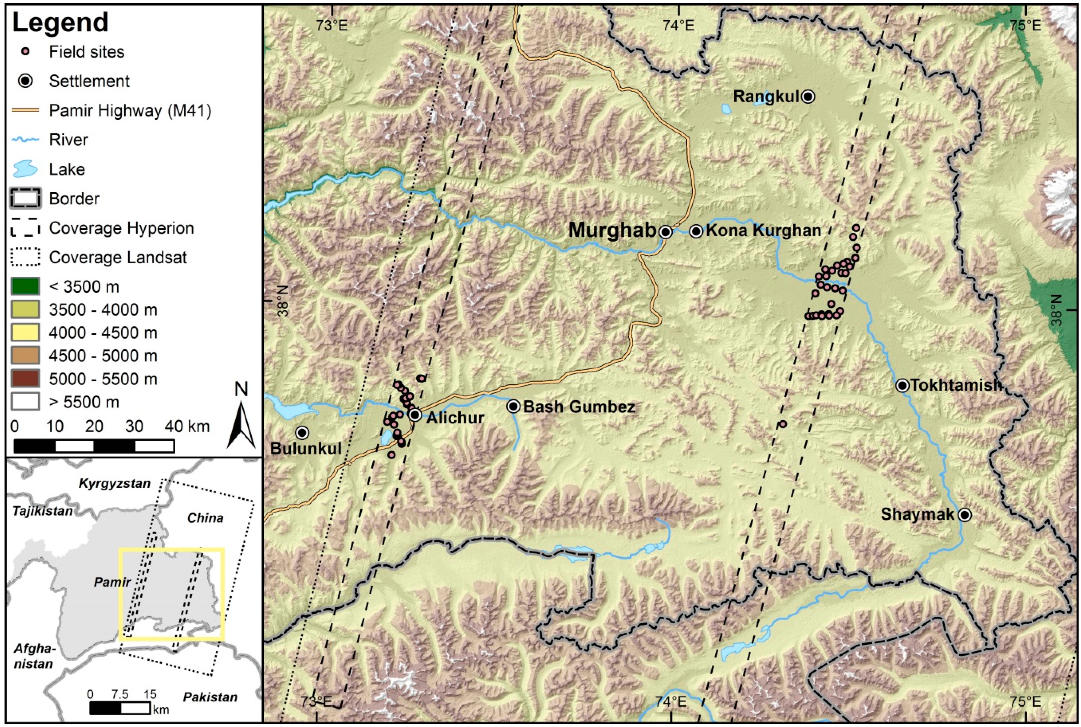
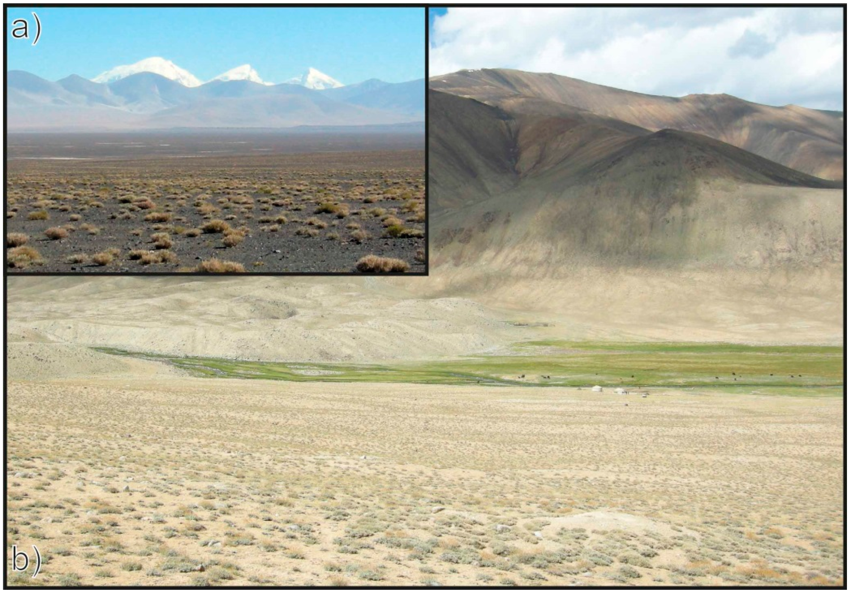
2.1. Research Area

The Eastern Pamirs of Tajikistan are a high mountain desert plateau with mean altitudes between 3500 and 5500 meters above sea level (Figure 1). The climate is characterized by low temperatures and scarce amounts of precipitation (Murghab annual mean 1998–2012: −1 °C, 94 mm, [18]). These natural conditions allow the development of dense, green grass vegetation only in areas with sufficient water supply (e.g., riparian vegetation in riverbeds, alpine meadows at very high altitudes). All other areas are sparsely covered and dominated by dwarf shrub vegetation adapted to water scarcity (Figure 2, [19]). These dwarf shrubs play a vital role in a region where the main economic activity is animal husbandry, as they serve both as a source of forage and fuel. The energy importance of shrubs is caused by the fact that they are the only local plants that develop woody parts, mainly in the root zone. Extensive harvesting, whereby the whole plant is dug up, has raised concerns regarding sustainable development of the region [19]. Therefore, a comprehensive assessment of the availability of this resource is needed as existing remote sensing approaches are still erroneous [4].

Figure 1. Overview of the research area, analyzed satellite images and field sites. The two Hyperion scenes were acquired on 3 August 2012 (western scene) and on 29 July 2013 (eastern scene), the Landsat OLI scene on 28 July 2013 respectively. DEM source: METI & NASA [20].

Figure 1. Overview of the research area, analyzed satellite images and field sites. The two Hyperion scenes were acquired on 3 August 2012 (western scene) and on 29 July 2013 (eastern scene), the Landsat OLI scene on 28 July 2013 respectively. DEM source: METI & NASA [20].

Figure 2. Photographs of (a) dwarf shrub stand located within the eastern Hyperion scene taken in fall 2014, and (b) dwarf shrub stand located within the western Hyperion scene with azonal grass vegetation in the background taken in summer 2013.

Figure 2. Photographs of (a) dwarf shrub stand located within the eastern Hyperion scene taken in fall 2014, and (b) dwarf shrub stand located within the western Hyperion scene with azonal grass vegetation in the background taken in summer 2013.

2.2. Data

Selection of satellite images was based on an acquisition date during the peak of the vegetation period to maximize the vegetation related reflectance signal in this arid environment [4].

2.2.1. Landsat OLI Data

A multispectral, terrain corrected image (L1T) with 30 m × 30 m spatial resolution was acquired on 28 July 2013 by the operational land imager (OLI) sensor of NASA’s Landsat 8 satellite. Visual inspection and comparison to GPS measurements showed that geo-referencing of the image was accurate and no further adjustment was needed. All eight multispectral bands were included in the analysis.

2.2.2. Hyperion Data

Two hyperspectral, terrain corrected images (Level 1T) with 30 m × 30 m spatial resolution were acquired on 3 August 2012 (western scene) and 29 July 2013 (eastern scene) by the Hyperion sensor of NASA’s Earth Observing 1 Satellite (Figure 1). The sensor spans the spectral range from 356–2577 nm with a bandwidth of ~10 nm leading to a total of 242 bands. Exclusion of bad bands (not calibrated, redundant, noise from atmospheric water vapor, low signal to noise ratio) left 158 bands for the analysis (cf. [21]). These are bands 8–57 (427–925 nm), 79–119 (933–1336 nm), 133–164 (1477–1790 nm), 183–184 (1982–1992 nm) and 188–220 (2032–2355 nm). Despite automatic terrain correction of Hyperion images, a spatial error was present in the data. This error was corrected by matching the image pixels with a nearest neighbor resampling algorithm to respective Landsat pixels using a second-order polynomial model with 19 control points (3 August 2012 RMSE_XY: 3.37 m, 29 July 2013 RMSE_XY: 5.02 m). The images were not corrected for other effects such as spectral smile or striping as no generally accepted procedure exists as well as to preserve the original spectral characteristics [22].

2.2.3. Atmospheric Correction

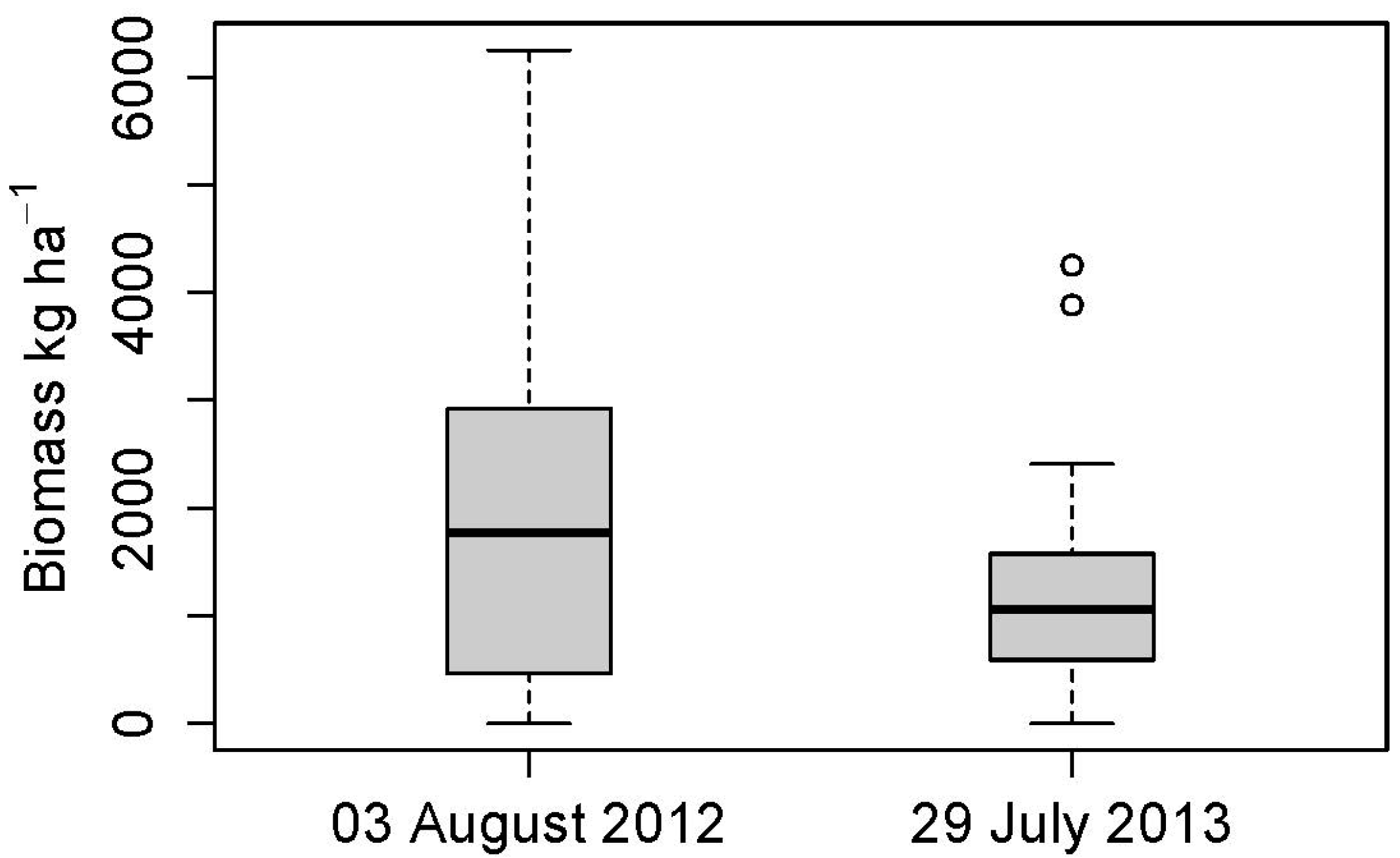
All images were recalculated to at-sensor radiance with subsequent atmospheric correction using ENVI’s state-of-the-art MODTRAN®-based FLAASH® approach. Aqua AIRS Level 3 Daily Standard Physical Retrieval product [23] provided information of daily atmospheric water vapor amounts for each scene to select the appropriate FLAASH® atmosphere.

2.2.4. Field Data

Sixty dwarf shrub stands (30 field sites in each Hyperion image) with homogenous vegetation cover and a minimum area of 60 m × 60 m were mapped in summer 2013 and fall 2014 with a handheld GPS device (horizontal RMSE ~5 m) using a study design similar to Zandler et al. [4]. Areas were selected preferentially to achieve the following objectives: (i) minimum size requirements [24]; (ii) mapping of a broad range of dwarf shrub densities; (iii) homogenous spectral properties and to take accessibility of field sites into account (cf. [4]). Furthermore, field sites were placed so that steep terrain is avoided to prevent potential spatial errors due to inaccurate terrain correction in Hyperion data. Within the stands, two subplots with 4 m side length were placed randomly and circumferences of all dwarf shrub individuals were measured inside the subplots. These measurements were used to calculate dwarf shrub total biomass using an allometric model developed specifically for the research area and the analyzed dwarf shrub species [4]. Results were averaged to represent the mean dwarf shrub biomass in kg∙ha⁻¹ of the stands. The midpoint between the subplots was taken as reference pixel to extract spectral information for each stand. A descriptive comparison of site biomass amounts shows that the western Hyperion scene is characterized by higher biomass amounts compared to the eastern scene (Figure 3).

Figure 3. Boxplots showing dwarf shrub biomass amounts of sites located in Hyperion scenes of August 2012 and July 2013, respectively. Each scene contains 30 field sites.

Figure 3. Boxplots showing dwarf shrub biomass amounts of sites located in Hyperion scenes of August 2012 and July 2013, respectively. Each scene contains 30 field sites.

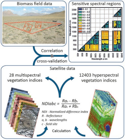
2.3. Spectral Index Computation and Statistical Analysis

Previous studies show that several spectral regions may be important in detecting different plant materials [7,25]. The most prominent is the red-infrared transition to analyze green vegetation [26] but many other spectral regions related to non-green, structural plant parts are mentioned as well [9,10,13,14,25,27,28,29,30]. For multispectral data, a very large number of vegetation indices potentially useful in detecting various plant tissues are available, but in the research area, most commonly used indices were shown to be unsuitable for biomass prediction [4]. Furthermore, existing hyperspectral indices designed to detect features of non-photosynthetic vegetation, may be inapplicable at low cover values on various soils [29]. Therefore, since there is no prior knowledge of hyperspectral indices that may be particularly suitable for biomass detection in the research area and to fully exploit the potential of the numerous Hyperion bands, all possible unique normalized difference indices (NDIs) were computed according to the formula:

$$NDIa,b,c=\frac{R{a}_c-R{b}_c}{R{a}_c+R{b}_c}$$

(1)

where R is reflectance, arranged in a descending order (2355–427 nm); a is the first wavelength and b is the reference wavelengths for field site c. This resulted in a total of 12,403 NDIs using Hyperion bands and 28 NDIs using Landsat OLI bands, respectively. These NDIs were grouped in four feature sets according to appearance of field sites in the two Hyperion scenes and based on the applied sensor: Western field sites (n = 30) within the Hyperion scene from 3 August 2012 (H2012), same field sites with Landsat data (LS2013a), eastern field sites (n = 30) within Hyperion scene from 29 July 2013 (H2013) and same field sites with Landsat data (LS2013b).

The features were paired in the correlation analysis with mean biomass of field sites as the response variable. Pearson’s correlation coefficient R was preferred based on preliminary studies showing a linear relationship of biomass and vegetation indices in the research area as well as visual inspection of a part of the present data [4]. Hypothesis testing to reject the null hypothesis of zero correlation results in a multiple testing problem. For instance, performing 10,000 independent hypothesis tests at the 5% level of significance would be expected to yield 500 false rejections if all null hypotheses are true. To address this problem, the Benjamini-Hochberg procedure [31], successfully applied by Peña et al. [21] in a comparable study, was used to control the false discovery rate (FDR) at a level of <5% and to compute adjusted p-value thresholds for each feature set.

Graphical displays were created for visual identification and comparison of spectral regions that are sensitive to dwarf shrub biomass amounts. Denomination of spectral regions follows Thenkabail et al. [12].

Similar to the multiple testing problem, the highest correlation coefficients obtained in a large family of correlations is not indicative of the predictive performance achieved in a situation where optimal indices are not known in advance and optimal index selection is therefore part of the data analysis process. To assess the performance of different sensors and feature sets in this situation and account for the high dimensionality of the data, we therefore used linear regression models built with a single stepwise forward variable selection step using Pearson’s correlation as the selection criterion. Larger models were not considered due to the small sample size. Predictive performances obtained for different feature sets and study areas were estimated using 100-repeated, 10-fold cross-validation. In this estimation method, the data set is randomly subdivided into 10 disjointed subsets or partitions. One partition at a time is used as the test set and the other 90% of the data as the training set in building a linear regression using the stepwise method. This procedure is repeated for each of the partitions and for 100 independent partitionings in total.

To evaluate feature sets, absolute root mean square error (RMSE), relative RMSE (RMSErel) and BIAS were calculated as:

$$\text{RMSE=}\sqrt{\begin{array}{c}\underset{\_}{{\displaystyle \sum }_{n=1}^n(Yi-\widehat{Yi})²}\\ n\end{array}}$$

(2)

$$\text{RMSErel}=\frac{RMSE}{\overline{Y}}\times 100\%$$

(3)

$$\text{BIAS}=\frac{1}{n}{\displaystyle \sum _{n=1}^n\widehat{Y}}i\text{-Yi}$$

(4)

where Yi is the measured and $\widehat{Yi}$ the predicted value of case i, $\overline{\text{Y}}$ is the observed mean value and n is the number of observations. Mean and standard deviation of these error measures over 100 cross-validation repetitions are reported.

3. Results

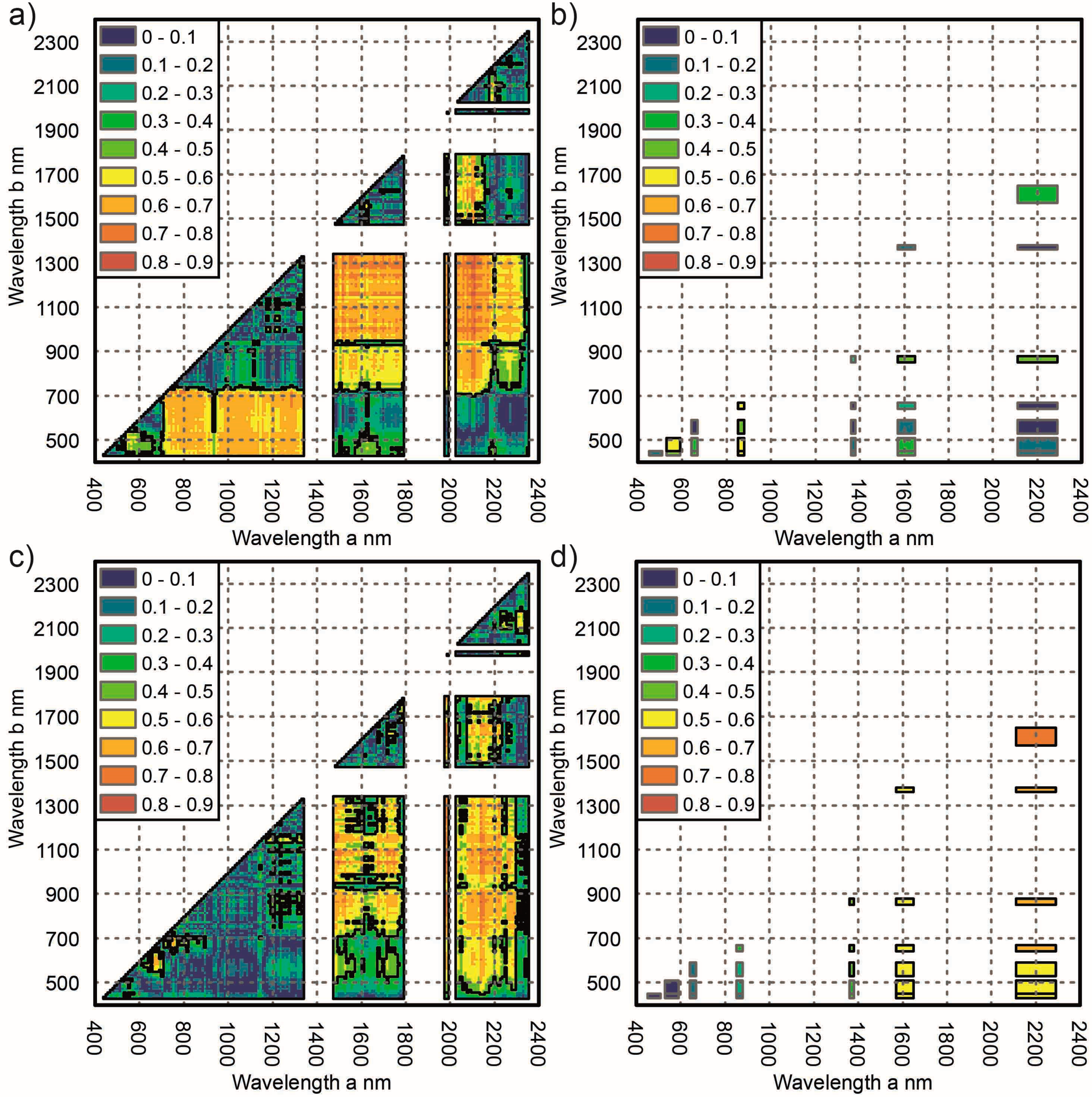
3.1. Visual Comparison of Biomass-Index Correlations

A broad range of spectral indices were significantly correlated with dwarf shrub biomass in both hyperspectral images (Figure 4). Comparison of feature sets showed substantial differences in correlation for indices calculated from green to far near infrared (FNIR) regions (500–1350 nm), where indices of H2012 resulted in a number of significant correlations in contrast to H2013 with almost no significant correlations in this spectral region. Indices derived from spectral bands in the early short-wave infrared (ESWIR, 1450–1800 nm) regions were more consistent as both H2012 and H2013 showed numerous strongly significant correlations in this domain. The closest match of results of the two feature sets was in the far short-wave infrared region (FSWIR), whereby strongest correlations of dwarf shrub biomass exist with indices of wavelengths 1950–2300 nm and associated reference wavelengths from 700 to 1800 nm.

A comparison of hyperspectral feature sets with multispectral feature sets and the same field sites showed similar correlations at related wavelengths. However, correlation coefficients of the hyperspectral feature sets were higher in most cases. Large differences were visible between the eastern multispectral feature set (LS2013b) with higher correlations in the ESWIR and FSWIR in contrast to the western multispectral feature set (LS2013a) with higher correlations in the green to near infrared (NIR) spectral regions.

Figure 4. Absolute values of Pearson’s correlation coefficients R of biomass with indices from field sites of feature sets (a) H2012, (b) LS2013a, (c) H2013, and (d) LS2013b. Black lines mark significant values controlled at a FDR < 5%.

Figure 4. Absolute values of Pearson’s correlation coefficients R of biomass with indices from field sites of feature sets (a) H2012, (b) LS2013a, (c) H2013, and (d) LS2013b. Black lines mark significant values controlled at a FDR < 5%.

3.2. Modeling Performance of Feature Sets

The western hyperspectral feature set (H2012) performed best in predicting dwarf shrub biomass according to the cross-validated modeling results with an RMSE of 1121 kg∙ha⁻¹, a RMSErel of 58% and an R² of 0.54 averaged over all repetitions (Table 1). The associated multispectral feature set (LS2013a) showed a higher RMSE of 1528 kg∙ha⁻¹ (RMSErel 78%) and lower R² of 0.15. Both models showed a relatively small bias. Eastern feature sets generally showed poor modeling performance ranging from RMSE values of 937–973 kg∙ha⁻¹ (77%–80% RMSErel) whereby the hyperspectral feature set (H2013) produced slightly lower values and higher R². Furthermore, model bias was higher for the eastern feature sets.

Table 1. Cross validated modeling performance of the different feature sets averaged over all repetitions.

	Modeled Mean RMSE (kg∙ha−1)	Modeled Mean R2	Modeled Mean Bias (kg∙ha−1)	Modeled Mean RMSErel (%)
Hyperion western sites (H2012)	1121	0.54	−23	58
Hyperion eastern sites (H2013)	937	0.29	69	77
Landsat OLI western sites (LS2013a)	1528	0.15	11	78
Landsat OLI eastern sites (LS2013b)	973	0.16	53	80

Table 1. Cross validated modeling performance of the different feature sets averaged over all repetitions.

	Modeled Mean RMSE (kg∙ha−1)	Modeled Mean R2	Modeled Mean Bias (kg∙ha−1)	Modeled Mean RMSErel (%)
Hyperion western sites (H2012)	1121	0.54	−23	58
Hyperion eastern sites (H2013)	937	0.29	69	77
Landsat OLI western sites (LS2013a)	1528	0.15	11	78
Landsat OLI eastern sites (LS2013b)	973	0.16	53	80

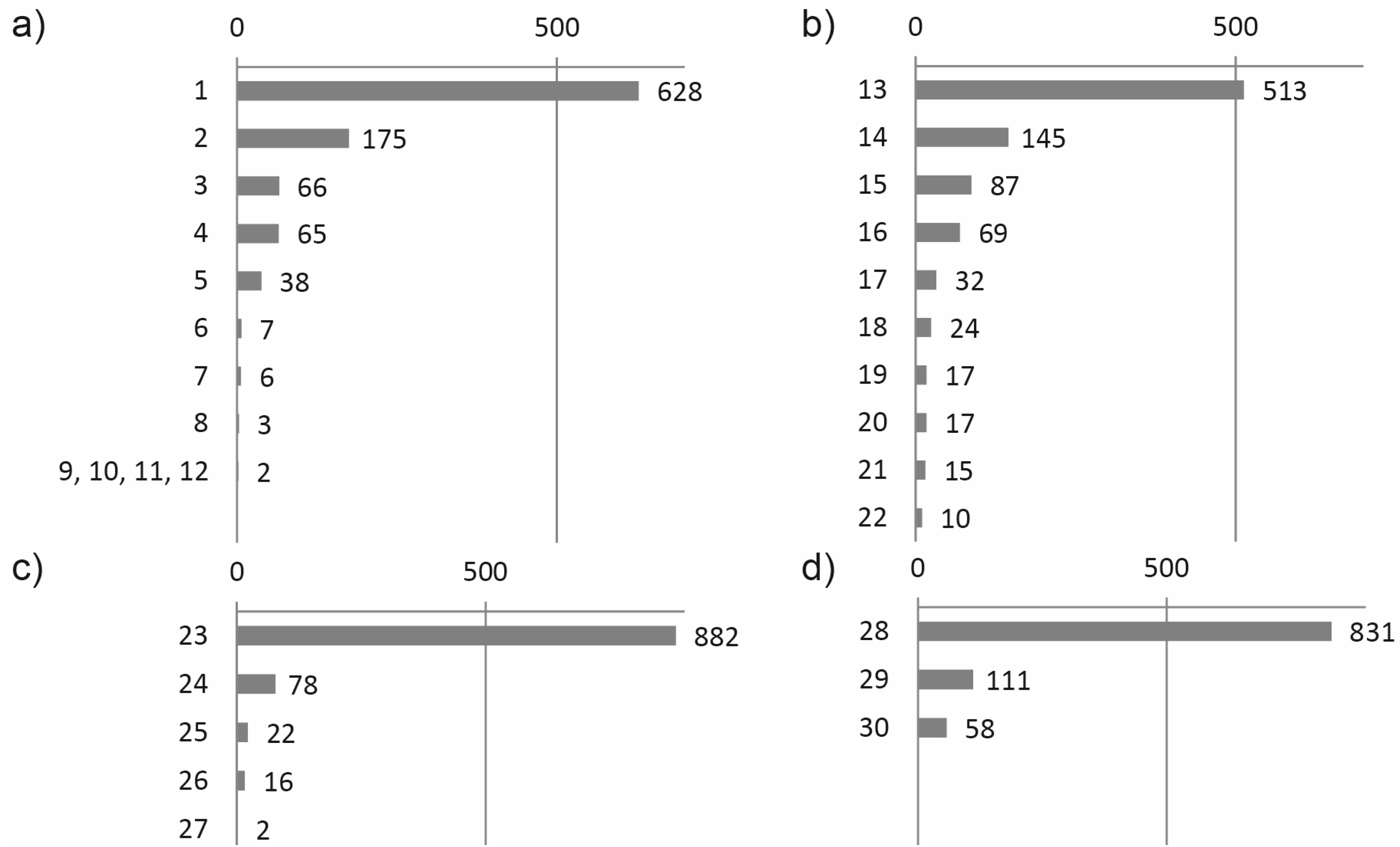
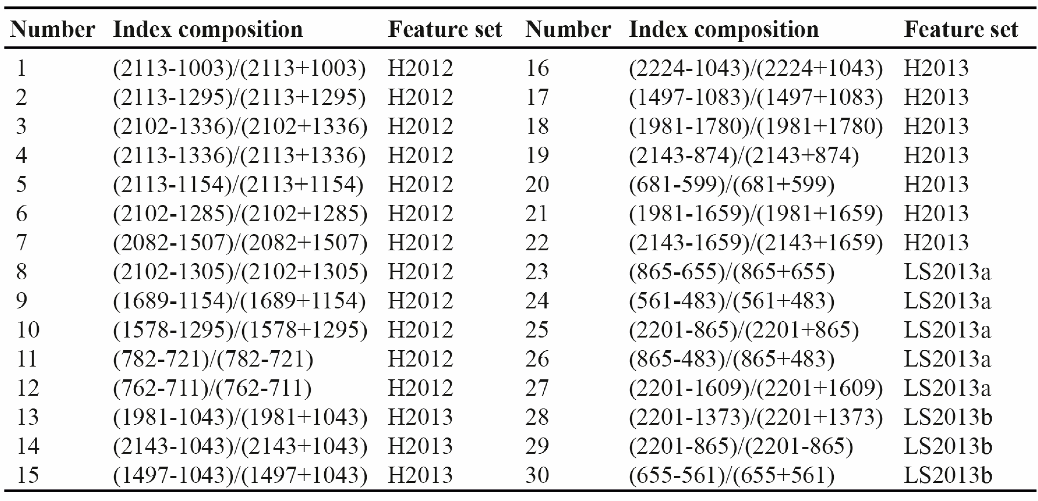
3.3. Variable Selection Frequency of Indices

Stepwise variable selection averaged over all folds and repetitions showed a considerably increased occurrence of the best performing NDI compared to other relevant indices over all feature sets (Figure 5). The best NDIs of the hyperspectral feature sets showed a strong concentration of FSWIR bands with reference wavelengths mostly from the FNIR to the ESWIR. Red–infrared and red edge indices were chosen rarely. The three most commonly selected NDIs of the western hyperspectral feature set H2012 all consisted of bands around 2100 nm with reference bands in the FNIR, whereas the eastern feature set H2013 showed higher diversification with bands from 1980–2140 nm and reference bands in the NIR. Little conformity was visible between hyperspectral and multispectral feature sets. A comparison of the multispectral feature sets showed large differences with an emphasis of the western feature set (LS2013a) on the red to infrared region, specifically the index calculated from wavelengths centered at 865 nm and 655 nm which is identical to the commonly known Normalized Difference Vegetation index (NDVI), in contrast to the most frequently selected NDI of the eastern feature set (LS2013b), which is composed of FSWIR and FNIR bands.

Figure 5. Occurrence of the 10 most frequently chosen NDIs according to stepwise variable selection from all folds and repetitions (1000 selections) with feature sets (a) H2012, (b) H2012, (c) LS2013a and (d) LS2013b.

Figure 5. Occurrence of the 10 most frequently chosen NDIs according to stepwise variable selection from all folds and repetitions (1000 selections) with feature sets (a) H2012, (b) H2012, (c) LS2013a and (d) LS2013b.

4. Discussion

4.1. Hyperspectral Indices for Dwarf Shrub Biomass Detection

This is the first study that addresses the sensitivity of hyperspectral narrow bands in the 400–2400 nm domain to dwarf shrub biomass in the research area, and to our knowledge, the first to analyze space-borne hyperspectral biomass detection in regions with cover values well below 20%. We showed that, even under these arid conditions, a great number of hyperspectral indices significantly correlate with dwarf shrub biomass quantities. Thereby, the green to NIR regions, which are commonly used for quantification of green cover, biomass, chlorophyll or leaf area index [7,8,9,12], were only partly correlated with biomass and did not constitute the indices with strongest correlations with the hyperspectral feature sets. Although the approximate red edge (700–780 nm), which is stressed as an important spectral region at low cover values in other studies [3,9,32], did show significant correlations with biomass amounts, it was not among the highest correlating hyperspectral indices.

However, high correlations commonly occurred in the ESWIR and FSWIR regions with both hyperspectral feature sets. These spectral domains are frequently mentioned as indicative of cellulose, lignin, wood or shrub material [7,8,10,13,25,27,28,29,30,33,34,35,36,37] and are therefore important for the detection of structural tissue. Especially the bands around 2020–2220 nm are considered as important for cellulose or lignin detection using remote sensing data [13,29,30,36,37] as they are distinctive from soil minerals and less affected by atmospheric gasses [37]. These results agree with the observed index selection frequencies where the three most important NDIs of H2012 consisted of bands with wavelength centers at 2113 nm or 2102 nm, and the second most important NDI of H2013 consisted of the band centered at 2143 nm. In previous studies, these bands were used for index computation to map crop residues with different reference wavelengths in the FSWIR [29,34,37]. The best performing NDI of H2013 utilized the wavelength centered at 1981 nm, a wavelength which may be sensitive to lignin, nitrogen [10,25] or plant residues [38]. Similarly, Oldeland et al. [11] state an importance of the SWIR spectral region for dry-matter analysis in an African savanna. Therefore, hyperspectral narrow-band NDIs, capturing spectral features of plant residues, lignin and cellulose, may also be instrumental in predicting dwarf shrub biomass in arid environments, as major parts of these plants consist of dry, non-green plant materials [4].

These results indicate that indices especially designed to separately capture the reflectance signal of cellulose in senescent vegetation, are suitable for biomass modeling in arid environments as well. However, correlation analysis of established indices for mapping senescent vegetation, like the Cellulose Absorption Index (CAI) or the Shortwave Infrared Normalized Difference Residue Index (SINDRI) as given in Serbin et al. [34], result only in weak significant correlations with CAI (Pearson’s correlation coefficients R 0.49 with H2012 and 0.47 with H2013) and no significant correlation of SINDRI with total biomass in our study. Similarly, the Normalized Difference Tillage Index (NDTI), whose equivalent showed a higher correlation only partly in our study (LS2013b), was not among the most important vegetation indices in modeling dwarf shrub biomass in previous research [4]. The reason for the higher correlations at the stated wavelengths may therefore not be a result of cellulose and lignin exclusively. Besides influence of aforementioned tissue, another reason for the importance of the ESWIR and FSWIR may be that green and woody parts of shrubs result in a strong contrast to the soil and so may have a strong influence in this spectral domain [13]. Additional research, incorporating field measured spectra of different plant materials, soils and various matter combined [13], could enhance knowledge on the nature of biomass reflectance properties and main influencing factors. However, regardless of the exact mechanisms and relative contributions of photosynthetic and non-photosynthetic tissue that may be the subject of additional research, the ESWIR and FSWIR spectral regions are more suitable for biomass detection compared to traditional red-infrared NDIs in our study and may supply important additional information in remote sensing based vegetation modeling in drylands.

4.2. Transferability of Spectral Indices Sensitive to Dwarf Shrub Biomass

An important objective of this study was the validity of spectral regions and indices to predict dwarf shrub biomass throughout different areas of the research area. While there was some agreement between the hyperspectral feature sets in the FSWIR, spectral regions of many NDIs that correlated strongly with dwarf shrub biomass and frequency of index selection differed noticeably between the feature sets. Therefore, a spatial generalization of specific narrow-band NDIs is difficult in this environment and individual model development is necessary. This is different to Thenkabail et al. [7], who report good agreement in optimal hyperspectral wavebands compared to other studies, but is in agreement with results obtained by Entcheva-Campbell et al. [22], who state that best performing hyperspectral NDIs for predicting ecosystem properties varied across sites. One reason for this lack in transferability of specific wavelengths may be the influence of non-constant factors that cannot fully be accounted for in correction algorithms [21]. Another reason may be a low signal-to-noise ratio characteristic of many Hyperion bands (cf. [27,32]) and apparent striping in the images. However, the broader 2100 nm region seems approximately transferable across hyperspectral sensors in this study, which is encouraging for future studies and indicates that an avoidance of indices based on too narrow bands may improve regional vegetation analysis [7].

The comparison of correlations and index selection frequencies of multispectral feature sets revealed a poor agreement in NDIs even though all field sites were situated in the same scene. An important reason may be the sensitivity of common broadband vegetation indices to background effects [39], like soil color, which emphasizes the importance of correction algorithms to account for these issues [4]. For example, NDVI values are especially sensitive to external interference at low vegetation cover values [40]. This may explain the importance of NDVI in the western data set with denser vegetation compared to its insignificance in the eastern data set with lower dwarf shrub cover. Another reason may be the diverse soil color prevalent in both feature sets, which is increasingly black in the eastern scene compared to a bright, brown-beige background in the western scene (Figure 2). In summary, the spatial transferability of spectral NDIs is challenging in the research area and this issue has to be considered in hyperspectral biomass modeling in drylands. These findings show that repeated variable assessment and model building is necessary in different regions and reveal the importance of knowledge discovery algorithms for advanced analysis procedures to handle huge hyperspectral datasets. However, the conformity of significant correlations comparing hyperspectral to multispectral feature sets with the same field sites suggests a high agreement at similar wavelengths between both sensors (cf. [41]).

4.3. Modeling Performance of Sensors

The hyperspectral Hyperion sensor showed increased performance in dwarf shrub biomass modeling compared to the Landsat OLI sensor. This has been previously shown by results obtained in different regions and from varying plant species [7,12,33,42] and suggests a large potential of hyperspectral sensors for vegetation analysis in arid environments as well. Furthermore, these results indicate that biomass quantification is possible even under the challenging conditions (noisy data, spectral variability) of applied, space-borne hyperspectral remote sensing in drylands within certain limits. This study supports the findings of Okin et al. [15], who showed that hyperspectral vegetation cover quantification in an arid region is possible under a best case scenario with a minimization of disturbing factors. However, in the eastern scene, which is characterized by lower biomass values, the performance of the hyperspectral sensor was only slightly better than the multispectral sensor. This demonstrates the limitations of hyperspectral-based vegetation analysis when cover values fall below a certain threshold. This is similar to results of Asner and Heidebrecht [32], who assert that accurate Hyperion-based vegetation quantification is only possible with denser vegetation. Finally, although the hyperspectral sensor outperformed the multispectral sensor in this study, results of biomass prediction are connected to major uncertainties and errors as well, which can be ascribed to the natural conditions of arid environments [15]. Nevertheless, extended modeling approaches, incorporating additional variables like topography [43], texture [44], soil and color-adjusted vegetation indices [40] as shown by Zandler et al. [4], using operational, widely available, space-borne hyperspectral data, can significantly reduce such errors in future applications. Furthermore, future research approaches may include variables particularly sensitive to photosynthetic vegetation, non-photosynthetic vegetation or both, in a multi variable-model after analyzing their relative contribution to the mixed biomass signal. Therefore, as is also expected by Asner and Green [2], this study suggests great potential for the upcoming products of new sensors like EnMAP or HyspIRI for future remote sensing based research of the world’s drylands.

5. Conclusions

This study showed that hyperspectral Hyperion data provides increased performance in predicting biomass in an arid environment compared to the multispectral sensor Landsat OLI. The reason is based on the higher spectral resolution, especially in the FSWIR, as highest correlations and best performing indices are situated in this region with the hyperspectral feature sets, whereby spectral regions intersecting with multispectral bands show similar correlations. The results indicate that sensors capturing spectral features of both green and woody material, which may be most distinctive in the FSWIR, are more suitable for biomass quantification in drylands that are characterized by plants consisting of non-photosynthetic parts to a large extent. Our research also revealed that spatial transferability of specific spectral indices is limited or not feasible, owing to the strong influence of background effects, underlining the importance of repeated model building and variable exploration in areas with different environmental conditions. Finally, substantial modeling errors were still present in all hyperspectral feature sets, which demonstrates the limitations of remote sensing based approaches and emphasizes the need for additional variables, such as texture or topography, for vegetation quantification in arid environments. However, the partly considerable modeling improvement with the hyperspectral sensor compared to the modern multispectral sensor in this arid setting indicates that upcoming, space-borne, operational hyperspectral sensors may enhance satellite-based vegetation analysis in drylands in the near future.

References

1. Sommer, S.; Zucca, C.; Grainger, A.; Cherlet, M.; Zougmore, R.; Sokona, Y.; Hill, J.; Della Peruta, R.; Roehrig, J.; Wang, G. Application of indicator systems for monitoring and assessment of desertification from national to global scales. Land Degrad. Dev. 2011, 22, 184–197. [Google Scholar] [CrossRef]
2. Asner, G.P.; Green, R. Imaging spectroscopy measures desertification in United States and Argentina. Eos Trans. AGU 2001, 82, 601–606. [Google Scholar] [CrossRef]
3. Eisfelder, C.; Kuenzer, C.; Dech, S. Derivation of biomass information for semi-arid areas using remote-sensing data. Int. J. Remote Sens. 2012, 33, 2937–2984. [Google Scholar] [CrossRef]
4. Zandler, H.; Brenning, A.; Samimi, C. Quantifying dwarf shrub biomass in an arid environment: Comparing empirical methods in a high dimensional setting. Remote Sens. Environ. 2015, 158, 140–155. [Google Scholar] [CrossRef]
5. Swatantran, A.; Dubayah, R.; Roberts, D.; Hofton, M.; Blair, J.B. Mapping biomass and stress in the Sierra Nevada using lidar and hyperspectral data fusion. Remote Sens. Environ. 2011, 115, 2917–2930. [Google Scholar] [CrossRef]
6. Schwieder, M.; Leitão, P.; Suess, S.; Senf, C.; Hostert, P. Estimating fractional shrub cover using simulated EnMAP data: A comparison of three machine learning regression techniques. Remote Sens. 2014, 6, 3427–3445. [Google Scholar] [CrossRef]
7. Thenkabail, P.S.; Enclona, E.A.; Ashton, M.S.; van der Meer, B. Accuracy assessments of hyperspectral waveband performance for vegetation analysis applications. Remote Sens. Environ. 2004, 91, 354–376. [Google Scholar] [CrossRef]
8. Lewis, M.; Jooste, V.; de Gasparis, A.A. Discrimination of arid vegetation with airborne multispectral scanner hyperspectral imagery. IEEE Trans. Geosci. Remote Sens. 2001, 39, 1471–1479. [Google Scholar] [CrossRef]
9. Elvidge, C.D.; Chen, Z.; Groeneveld, D.P. Detection of trace quantities of green vegetation in 1990 AVIRIS data. Remote Sens. Environ. 1993, 44, 271–279. [Google Scholar] [CrossRef]
10. Serrano, L.; Penuelas, J.; Ustin, S.L. Remote sensing of nitrogen and lignin in Mediterranean vegetation from AVIRIS data: Decomposing biochemical from structural signals. Remote Sens. Environ. 2002, 81, 355–364. [Google Scholar] [CrossRef]
11. Oldeland, J.; Dorigo, W.; Wesuls, D.; Jürgens, N. Mapping bush encroaching species by seasonal differences in hyperspectral imagery. Remote Sens. 2010, 2, 1416–1438. [Google Scholar] [CrossRef]
12. Thenkabail, P.S.; Mariotto, I.; Gumma, M.K.; Middleton, E.M.; Landis, D.R.; Huemmrich, K.F. Selection of hyperspectral narrowbands (HNBs) and composition of hyperspectral twoband vegetation indices (HVIs) for biophysical characterization and discrimination of crop types using field reflectance and Hyperion/EO-1 data. IEEE J. Sel. Top. Appl. Earth Obs. Remote Sens. 2013, 6, 427–439. [Google Scholar] [CrossRef]
13. Asner, G.P.; Wessman, C.A.; Bateson, C.; Privette, J.L. Impact of tissue, canopy, and landscape factors on the hyperspectral reflectance variability of arid ecosystems. Remote Sens. Environ. 2000, 74, 69–84. [Google Scholar] [CrossRef]
14. Oldeland, J.; Dorigo, W.; Lieckfeld, L.; Lucieer, A.; Jürgens, N. Combining vegetation indices, constrained ordination and fuzzy classification for mapping semi-natural vegetation units from hyperspectral imagery. Remote Sens. Environ. 2010, 114, 1155–1166. [Google Scholar] [CrossRef]
15. Okin, G.S.; Roberts, D.A.; Murray, B.; Okin, W.J. Practical limits on hyperspectral vegetation discrimination in arid and semiarid environments. Remote Sens. Environ. 2001, 77, 212–225. [Google Scholar] [CrossRef]
16. Vanselow, K.A. The High-Mountain Pastures of the Eastern Pamirs (Tajikistan): An Evaluation of the Ecological Basis and the Pasture Potential. Ph.D. Thesis, Friedrich Alexander University, Erlangen-Nuremberg, Germany, 2011. [Google Scholar]
17. Vanselow, K.; Samimi, C. Predictive mapping of dwarf shrub vegetation in an arid high mountain ecosystem using remote sensing and random forests. Remote Sens. 2014, 6, 6709–6726. [Google Scholar] [CrossRef]
18. Tajik Met Service, Dushanbe, Tajikistan. Climatic data for the Pamir Region. 2013.
19. Kraudzun, T.; Vanselow, K.A.; Samimi, C. Realities and myths of the Teresken Syndrome—An evaluation of the exploitation of dwarf shrub resources in the Eastern Pamirs of Tajikistan. J. Environ. Manage. 2014, 132, 49–59. [Google Scholar] [CrossRef] [PubMed]
20. Aster Global Digital Elevation Model, version V002; NASA LP DAAC/U.S. Geological Survey: Sioux Falls, SD, USA, 2009.
21. Peña, M.A.; Brenning, A.; Sagredo, A. Constructing satellite-derived hyperspectral indices sensitive to canopy structure variables of a Cordilleran Cypress (Austrocedrus chilensis) forest. ISPRS J. Photogramm. Remote Sens. 2012, 74, 1–10. [Google Scholar] [CrossRef]
22. Campbell, P.K.E.; Middleton, E.M.; Thome, K.J.; Kokaly, R.F.; Huemmrich, K.F.; Lagomasino, D.; Novick, K.A.; Brunsell, N.A. EO-1 Hyperion reflectance time series at calibration and validation sites: Stability and sensitivity to seasonal dynamics. IEEE J. Sel. Top. Appl. Earth Obs. Remote Sens. 2013, 6, 276–290. [Google Scholar] [CrossRef]
23. Aqua AIRS Level 3 Daily Standard Physical Retrieval (AIRS+AMSU), version 006; NASA Goddard Earth Science Data and Information Services Center (GES DISC): Greenbelt, MD, USA, 2013.
24. Justice, C.O.; Townshend, J.G. Integrating ground data with remote sensing. In Terrain Analysis and Remote Sensing; Townshend, J.G., Ed.; Allen and Unwin: London, UK, 1981; pp. 38–58. [Google Scholar]
25. Fourty, T.; Baret, F.; Jacquemoud, S.; Schmuck, G.; Verdebout, J. Leaf optical properties with explicit description of its biochemical composition: Direct and inverse problems. Remote Sens. Environ. 1996, 56, 104–117. [Google Scholar] [CrossRef]
26. Chen, Z.; Elvidge, C.D.; Groeneveld, D.P. Monitoring seasonal dynamics of arid land vegetation using AVIRIS data. Remote Sens. Environ. 1998, 65, 255–266. [Google Scholar] [CrossRef]
27. Martin, M.E.; Aber, J.D. High spectral resolution remote sensing of forest canopy lignin, nitrogen, and ecosystem processes. Ecol. Appl. 1997, 7, 431–443. [Google Scholar] [CrossRef]
28. Takahashi, T.; Yasuoka, Y.; Fujii, T. Hyperspectral remote sensing of riparian vegetation and leaf chemistry contents. In Proceedings of 23rd Asian Conference on Remote Sensing, Kathmandu, Nepal, 25–29 November 2002.
29. Nagler, P.L.; Inoue, Y.; Glenn, E.; Russ, A.; Daughtry, C.S. Cellulose absorption index (CAI) to quantify mixed soil–plant litter scenes. Remote Sens. Environ. 2003, 87, 310–325. [Google Scholar] [CrossRef]
30. Daughtry, C.S. Discriminating crop residues from soil by shortwave infrared reflectance. Agron. J. 2001, 93, 125–131. [Google Scholar] [CrossRef]
31. Benjamini, Y.; Hochberg, Y. Controlling the false discovery rate: A practical and powerful approach to multiple testing. J. R. Stat. Soc. Ser. B Methodol. 1995, 57, 289–300. [Google Scholar]
32. Asner, G.P.; Heidebrecht, K.B. Imaging spectroscopy for desertification studies: Comparing AVIRIS and EO-1 Hyperion in Argentina drylands. IEEE Trans. Geosci. Remote Sens. 2003, 41, 1283–1296. [Google Scholar] [CrossRef]
33. Thenkabail, P.S.; Enclona, E.A.; Ashton, M.S.; Legg, C.; De Dieu, M.J. Hyperion, IKONOS, ALI, and ETM+ sensors in the study of African rainforests. Remote Sens. Environ. 2004, 90, 23–43. [Google Scholar] [CrossRef]
34. Serbin, G.; Hunt, E.R., Jr.; Daughtry, C.S.T.; McCarty, G.W.; Doraiswamy, P.C. An improved ASTER index for remote sensing of crop residue. Remote Sens. 2009, 1, 971–991. [Google Scholar] [CrossRef]
35. Elvidge, C.D. Visible and near infrared reflectance characteristics of dry plant materials. Int. J. Remote Sens. 1990, 11, 1775–1795. [Google Scholar] [CrossRef]
36. Elvidge, C.D. Examination of the spectral features of vegetation in 1987 AVIRIS data. In Proceedings of the First AVIRIS Performance Evaluation Workshop, Pasadena, CA, USA, 6–8 June 1988; Jet Propulsion Laboratory: Pasadena, CA, USA, 1988; pp. 97–101. [Google Scholar]
37. Serbin, G.; Daughtry, C.S.T.; Hunt, E.R.; Reeves, J.B.; Brown, D.J. Effects of soil composition and mineralogy on remote sensing of crop residue cover. Remote Sens. Environ. 2009, 113, 224–238. [Google Scholar] [CrossRef]
38. Singh, R.B.; Ray, S.S.; Bal, S.K.; Sekhon, B.S.; Gill, G.S.; Panigrahy, S. Crop residue discrimination using ground-based hyperspectral data. J. Indian Soc. Remote Sens. 2013, 41, 301–308. [Google Scholar]
39. Schmidt, H.; Karnieli, A. Sensitivity of vegetation indices to substrate brightness in hyper-arid environment: The Makhtesh Ramon Crater (Israel) case study. Int. J. Remote Sens. 2001, 22, 3503–3520. [Google Scholar]
40. Bannari, A.; Morin, D.; Bonn, F.; Huete, A.R. A review of vegetation indices. Remote Sens. Rev. 1995, 13, 95–120. [Google Scholar] [CrossRef]
41. Thome, K.J.; Biggar, S.F.; Wisniewski, W. Cross comparison of EO-1 sensors and other earth resources sensors to Landsat-7 ETM+ using Railroad Valley Playa. IEEE Trans. Geosci. Remote Sens. 2003, 41, 1180–1188. [Google Scholar] [CrossRef]
42. Mariotto, I.; Thenkabail, P.S.; Huete, A.; Slonecker, E.T.; Platonov, A. Hyperspectral versus multispectral crop-productivity modeling and type discrimination for the HyspIRI mission. Remote Sens. Environ. 2013, 139, 291–305. [Google Scholar] [CrossRef]
43. Sternberg, M.; Shoshany, M. Influence of slope aspect on Mediterranean woody formations: Comparison of a semiarid and an arid site in Israel. Ecol. Res. 2001, 16, 335–345. [Google Scholar] [CrossRef]
44. Sarker, L.R.; Nichol, J.E. Improved forest biomass estimates using ALOS AVNIR-2 texture indices. Remote Sens. Environ. 2011, 115, 968–977. [Google Scholar] [CrossRef]