Regional Leaf Area Index Retrieval Based on Remote Sensing: The Role of Radiative Transfer Model Selection

Abstract

Physically-based approaches for estimating Leaf Area Index (LAI) using remote sensing data rely on radiative transfer (RT) models. Currently, many RT models are freely available, but determining the appropriate RT model for LAI retrieval is still problematic. This study aims to evaluate the necessity of RT model selection for LAI retrieval and to propose a retrieval methodology using different RT models for different vegetation types. Both actual experimental observations and RT model simulations were used to conduct the evaluation. Each of them includes needleleaf forests and croplands, which have contrasting structural attributes. The scattering from arbitrarily inclined leaves (SAIL) model and the four-scale model, which are 1D and 3D RT models, respectively, were used to simulate the synthetic test datasets. The experimental test dataset was established through two field campaigns conducted in the Heihe River Basin. The results show that the realistic representation of canopy structure in RT models is very important for LAI retrieval. If an unsuitable RT model is used, then the root mean squared error (RMSE) will increase from 0.43 to 0.60 in croplands and from 0.52 to 0.63 in forests. In addition, an RT model’s potential to retrieve LAI is limited by the availability of a priori information on RT model parameters. 3D RT models require more a priori information, which makes them have poorer generalization capability than 1D models. Therefore, physically-based retrieval algorithms should embed more than one RT model to account for the availability of a priori information and variations in structural attributes among different vegetation types.

1. Introduction

Leaf Area Index (LAI) influences vegetation photosynthesis, transpiration and the energy balance of the land surface; it is therefore among the essential inputs of climate, hydrology and ecosystem productivity models [1]. Some LAI products have been generated based on remote sensing (RS), for example, the four-day/eight-day 1-km MODIS product [2], the 10-day 1-km GEOV1 product [3], the 10-day 1-km CYCLOPES product [4], the 16-day 0.01° JRC-TIP product [5], the eight-day 5-km/1-km GLASS product [6] and the monthly 1-km GLOBCARBON product [7]. However, recent validation activities have shown that the current LAI products are still unable to meet the requirements of many applications [8,9]. The factors that influence the accuracy of LAI products mainly include radiative transfer (RT) model uncertainty, the accuracy of the inversion method, the quantity and uncertainty of the RS measurements and spatial heterogeneity within the footprint of pixels [10,11]. With the continuing improvement of the quality of reflectance products, the lack of sufficient observations becomes a crucial limiting factor, particularly in equatorial and high-latitude regions, because of high cloud coverage. The concurrent use of data from several satellite systems can increase the observing frequency and mitigate this limitation [12]. Therefore, RT model accuracy is important for further improving the accuracy of LAI products [13].

There are two main types of approaches to estimate LAI from RS data: empirical approaches and physically-based approaches [14,15]. Empirical approaches rely on the statistical relationships between LAI and RS data. These approaches are computationally efficient, but are site-, species-, time- and sensor-specific [16,17]. Physically-based approaches rely on the inversion of RT models. RT models summarize the knowledge of the physical processes involved in the photon transport within vegetation canopy [18]. Therefore, physically-based approaches can be adapted for various conditions [2,7]. Different strategies have been proposed for the inversion of the RT model, including conventional numerical optimization methods [19] and look-up table (LUT) techniques [2]. Recently, hybrid approaches, in which LUTs are generated to feed machine learning approaches, have been increasingly utilized [20,21]. These approaches are facilitated by the rapid development in the field of machine learning, and increasingly, more advanced machine learning approaches are applied for estimating LAI, such as Gaussian process regression [22,23] and dynamic Bayesian networks [24,25]. One of the main difficulties in physically-based approaches is the ill-posedness of the inversion. Several regularization methods can be implemented to reduce the drawback of ill-posedness: model coupling [26], using a priori information [27], spatial constraints [28,29], temporal constraints [30] and combined spatio-temporal constraints [31].

In physically-based approaches, model uncertainty is significantly related to the manner in which the canopy architecture is represented in canopy RT models. According to the method used to characterize structural properties, canopy RT models can be grouped into two categories: (1) one-dimensional (1D) models that describe the canopy as a horizontally homogeneous and semi-infinite layer; and (2) three-dimensional (3D) models that are capable of resolving individual tree crowns [32]. The structural representations of different types of vegetation vary widely. To the best of our knowledge, there is no universal canopy RT model suitable for all canopies. Therefore, different RT models are needed for different types of vegetation [33]. Widlowski et al. [34] found that the reflectance simulated by 1D and 3D models tends to converge at resolutions beyond 100 m. In this sense, when retrieving LAI using medium- or coarse-resolution RS data (e.g., MODIS, VEGETATION or AVHRR), 3D models may over-interpret the measured reflectance; because in this case, 3D RT models perform similarly to 1D models in accounting for the measured reflectance, but they require more a priori information. Nevertheless, it was also demonstrated in some studies [35,36] that the misrepresentation of structural properties within the stand scale may cause the retrieved parameters to diverge from the true values. Therefore, the RT model selection may have profound implications on LAI retrieval. However, for operational feasibility, the current LAI products are all based on a single model. For example, MODIS [2], GLOBCARBON [7], CYCLOPES [4] and JRC-TIP [5] LAI products use the stochastic radiative transfer model [37], the four-scale model [38], the scattering from arbitrarily inclined leaves (SAIL) model [39] and the two-stream model [40,41], respectively. The MODIS and GLOBCARBON retrieval algorithms also use land cover maps as a priori information to constrain the parameter space, but not for model selection.

Physically-based approaches for estimating LAI rely on RT models. Currently, many RT models are freely available, but determining the appropriate RT model for LAI retrieval is still problematic. The objective of this study is to evaluate the impact of RT model selection on LAI retrieval. To this end, a hybrid inversion approach was developed to estimate LAI using both the SAIL and four-scale models. The retrieval results obtained from the two RT models were compared with the reference LAI to quantitatively analyze the influence of RT model selection. The paper is organized as follows: Section 2 describes the method used for the evaluation. The experimental and synthetic test datasets generated through field campaigns and RT model simulations are outlined in Section 3. Section 4 presents the results and discusses the main findings. Finally, the conclusions are presented in Section 5.

2. Methodology

2.1. Retrieving LAI Using Different RT Models

The structure of the vegetation canopy determines the magnitude and angular distribution of the canopy-leaving radiation; its parameterization is therefore one of the most important components of RT models [37]. In early RT models, the canopy structure was assumed to be horizontally homogeneous and mainly characterized by leaf inclination angle distribution and leaf area volume density [39]. However, actual vegetation generally shows different degrees of spatial heterogeneity, which manifests as clumping effects at multiple scales: shoot scale [35], between-crown scale [42] and landscape scale [10,11]. Generally, no universal RT model is suitable for characterizing all scales of structural properties. Although computer simulation models [43,44] are designed for different kinds of scenes, they cannot be straightforwardly used for LAI retrieval, because of their computational intensiveness. Theoretically, 1D RT models are applied to horizontally homogeneous vegetation, which is treated as a plane-parallel “cloud of leaves” rather than individually distinguishable plant. Grasses and croplands (at the later growth stage) are generally treated as this type of vegetation [33,45]. In 3D RT models, the canopy is assumed to be composed of many discrete crowns. These RT models are appropriate for vegetation characterized by horizontal heterogeneity, for example savannas and forests [37,38].

Land cover maps have been operationally used in LAI retrieval algorithms. For model selection, the global land cover needs to be stratified according to canopy structural differences. Therefore, traditional land cover classifications based on ecological or functional metrics may be unsuitable. In this study, the third classification system of the MODIS land cover product (MCD 12Q1) was used to select appropriate RT models. In MCD 12Q1, the global vegetation is stratified into six canopy architectural types: grasses and cereal crops, shrubs, broadleaf crops, savannas, broadleaf forests and needle forests [46]. These types are structurally variable in the horizontal and vertical dimensions, but the structural properties of a specific type are considered similar. The use of this classification system implies that the landscape within the footprint of a pixel, 500 m in this study, can be translated to one of the six types. The early version of the classification system was used. In the latest version, broadleaf/needleleaf forests are subdivided into evergreen and deciduous forests, but each subcategory has nearly identical canopy structure properties (with different leaf optical properties) [2]. The canopy structural attributes and the recommended RT models of the six vegetation types are as in Table 1.

Table 1. Canopy structural attributes of different land covers and the corresponding recommended RT models suitable for Leaf Area Index (LAI) retrieval.

	Grasses and Cereal Crops	Shrubs	Broadleaf Crops	Savannas	Broadleaf Forests	Needle Forests
Horizontal heterogeneity	variable	yes	variable	yes	yes	yes
Ground cover	10%–100%	20%–60%	10%–100%	20%–40%	>70%	>70%
Vertical heterogeneity	no	no	no	yes	yes	yes
Recommended RT model	1D for grasses and cereal crops dependent on the growth stage	3D	dependent on the growth stage	3D	3D	3D

Table 1. Canopy structural attributes of different land covers and the corresponding recommended RT models suitable for Leaf Area Index (LAI) retrieval.

	Grasses and Cereal Crops	Shrubs	Broadleaf Crops	Savannas	Broadleaf Forests	Needle Forests
Horizontal heterogeneity	variable	yes	variable	yes	yes	yes
Ground cover	10%–100%	20%–60%	10%–100%	20%–40%	>70%	>70%
Vertical heterogeneity	no	no	no	yes	yes	yes
Recommended RT model	1D for grasses and cereal crops dependent on the growth stage	3D	dependent on the growth stage	3D	3D	3D

(1)

Grasses and cereal crops: Grasses are vertically and horizontally homogeneous, and the vegetation ground cover is approximately 100%. A 1D RT model is recommended. The foliage clumping can be accounted for by simply introducing the clumping index when forcing the RT model [47]. For cereal crops, large variations exist in vegetation ground cover from crop planting (10%) to maturity (100%). At least two types of RT models should be adopted at different growth stages, i.e., the row structure model for the early growth stage and a 1D RT model for the later growth stage [33].

(2)

Shrubs: horizontal heterogeneity, low (20%) to intermediate (60%) vegetation ground cover. A 3D RT model is recommended [37,38].

(3)

Broadleaf crops: Large variations in vegetation ground cover from crop planting (10%) to maturity (100%). At least two types of RT models should be adopted at different growth stages, i.e., the row structure model for the early growth stage and a 1D RT model for the later growth stage [33].

(4)

Savanna: Two distinct vertical layers of a grass understory and low ground cover of overstory trees (20%–40%); the canopy optics and structure are therefore vertically heterogeneous. A 3D RT model is recommended [37,38].

(5)

Broadleaf forests: vertical and horizontal heterogeneity and high ground cover. A 3D RT model is recommended [37,38].

(6)

Needleleaf forests: Most heterogeneous, with high ground cover. A 3D RT model is recommended [37,38].

To evaluate the necessity of the RT model selection, we chose two biomes with contrasting structural attributes: croplands and needleleaf forests. In addition, two RT models were selected in this study: the SAIL model [39] and the four-scale model [38]. They are representatives of 1D and 3D RT models, respectively. In the SAIL model, canopy structure is characterized by LAI, the average leaf angle inclination (ALA) and the hot spot parameter (H). The four-scale model simulates the reflectance based on canopy architecture at four scales: (1) crown groups; (2) crown geometry; (3) branches; and (4) foliage elements. The canopy structure parameters can be separated into two categories: (1) site parameter, including quadrat size (Q_z), LAI, tree density (T_d), cluster mean size (m2); and (2) tree architecture parameters (the crown is assumed to be a cone + a cylinder in this study), including crown radius (r), height of trunk (h_a) and cylinders (h_b), half apex angle (α), needle to shoot ratio (γ_E), foliage clumping index (Ω_E), mean width of element shadows cast inside tree crowns (W_s) and leaf inclination angle distribution function (LIAD).

2.2. The Neural Network Inversion Technique

The neural network (NN) approach was selected to invert the RT models, because of its computational efficiency and ideal interpolation capacity [48]. Two feedforward NNs (denoted as SAILNN and four-scaleNN) were trained based on the corresponding training datasets. They have identical architectures: the input layer has five neurons, which correspond to reflectances in the red and near-infrared bands, solar zenith angle, sensor zenith angle and relative azimuth angle between the Sun and sensor, respectively. A hidden layer comprises 8 tangent sigmoid neurons. The single output is LAI, and the linear transfer function is used in the output layer. This architecture was established by a trial-and-error approach. The Levenberg–Marquardt optimization algorithm [49] was used to adjust the synaptic weights and neuron bias to obtain the best agreement between the output simulated by the NN and the corresponding value of LAI in the training dataset. After calibration, the two NNs (SAILNN and four-scaleNN) were applied to the MODIS daily surface reflectance products (MOD09GA) [50] to produce two LAI maps, denoted as SAIL LAI and four-scale LAI, respectively.

2.3. Evaluation Criteria

To analyze the influence of RT model selection, we compared the retrieval results from the two RT models with the in situ measured LAI. The RT models’ performance was evaluated with the root mean squared error (RMSE) to assess accuracy and the coefficient of determination (R²) to account for the goodness-of-fit. To quantitatively analyze the impact of RT model selection on regional LAI spatial variability characterization, the Kullback–Leibler (K-L) divergence was calculated,

$$D_{KL}\left(P\mathrm{||}Q\right)={\displaystyle \int \ln \left(\frac{p\left(x\right)}{q\left(x\right)}\right)p\left(x\right)}\text{d}x$$

(1)

where P and Q are the probability distributions of a random variable X, i.e., LAI in this study, and p(x) and q(x) indicate the densities of P and Q at x. The K-L divergence of Q from P, denoted as D_KL(P||Q), is a measure of the information loss when Q is used to approximate P [51]. A larger K-L divergence corresponds to greater information loss, and vice versa.

3. Experimental and Synthetic Datasets

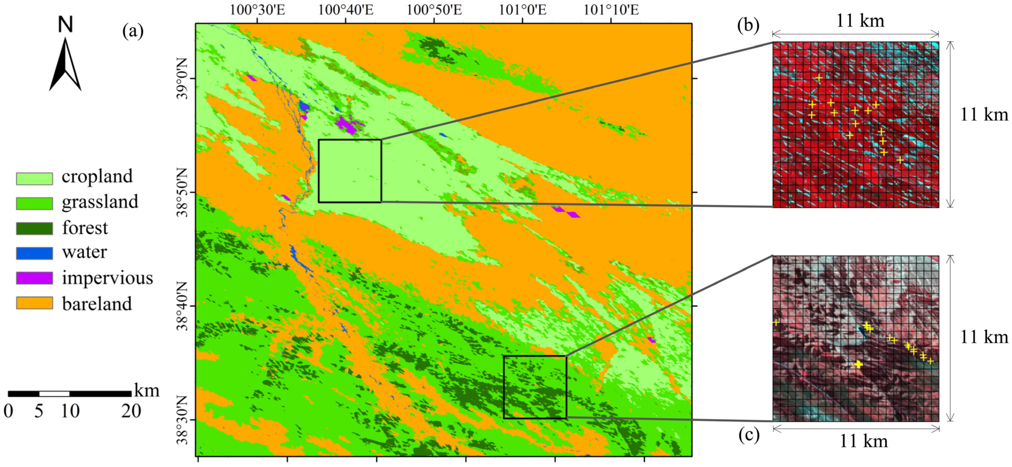
The impact of RT model selection on LAI retrieval was evaluated over both experimental and synthetic test datasets, including the top-of-canopy (TOC) reflectance and the corresponding LAI. The experimental test dataset was acquired through two field campaigns (in forests and croplands, respectively) carried out in the Heihe River Basin, China. The synthetic test dataset was generated with simulations of the four-scale and SAIL models, corresponding to the experimental test dataset, to complement the evaluation and to analyze in a controlled environment.

3.1. Study Area

The Heihe River Basin, located between 97°24′–102°10′E and 37°41′–42°42′N, is China’s second largest inland river basin. A comprehensive watershed-scale RS campaign, called Watershed Allied Telemetry Experimental Research (WATER) [52], and its successor, Heihe Watershed Allied Telemetry Experimental Research (HiWater) [53], have been carried out in this typical inland river basin since 2008. These campaigns equipped the Heihe River Basin with good research facilities and rich datasets [54]. In WATER, three key experimental areas were identified: a cold region experimental area, an arid region experimental area (AREA) and a forest experimental area (FEA), to represent three key types of hydrologic processes. In this study, two 11 × 11 km sub-regions in the latter two key experimental areas were selected as our study area (Figure 1).

The AREA sub-region (Figure 1b) is located in the middle reaches of the Heihe River Basin. The terrain is very flat, with an elevation ranging from 1500 to 2000 m. The annual precipitation is less than 200 mm. In this sub-region, croplands are the main land cover type, and the primary crop species are wheat and maize. The sub-region in FEA (Figure 1c) is located in the Qilian Mountains. Forests, dominated by Picea crassifolia, are widely distributed at elevations between 2800 and 3500 m.

Figure 1. Land cover map of the upper and middle reaches of the Heihe River Basin in China (a) and the locations of the arid region experimental area (AREA) (b) and the forest experimental area (FEA) (c) sub-regions. The land cover map was downloaded from [55]. (b,c) False color images of ASTER/ETM+ acquired on 10 July 2012 and 28 May 2008, respectively. The black boxes and yellow crosses in (b) and (c) display the MODIS 500-m grids and field sampling plots.

Figure 1. Land cover map of the upper and middle reaches of the Heihe River Basin in China (a) and the locations of the arid region experimental area (AREA) (b) and the forest experimental area (FEA) (c) sub-regions. The land cover map was downloaded from [55]. (b,c) False color images of ASTER/ETM+ acquired on 10 July 2012 and 28 May 2008, respectively. The black boxes and yellow crosses in (b) and (c) display the MODIS 500-m grids and field sampling plots.

3.2. Experimental Test Dataset

3.2.1. Ground Measurements

Two field campaigns were carried out from 2 to 8 June 2008 and 13 July 2012 in the FEA and AREA sub-regions, respectively. The field sampling plots within the two 11 × 11 km areas are displayed in Figure 1b,c. The sampling was designed to represent the vegetation variability within each sub-region while minimizing field measurement efforts. There are 19 and 14 plots in FEA and AREA, respectively, and each plot contains 12 samples. At the plot scale, the measurements were distributed along two perpendicular 20-m transects (with measurement points located at 4-m intervals), as recommended by the Validation of Land European RS Instruments (VALERI) network [56]. Two LAI-2000 instruments were operated simultaneously. One was located below the canopy, and the other was located in an open area nearby. The measurements were obtained during overcast sky or in early morning or late evening to avoid sun flecks. The LAI was calculated from the canopy gap fraction value. The effective LAI rather than true LAI was used when establishing the experimental test dataset, because it is better correlated with the RS observations [57] and optical field measurements [58]. Although it is theoretically possible to estimate the true LAI from effective LAI, in reality, this is a complicated process and was not attempted in the generation of the experimental test datasets. The field-measured values of LAI vary between 0.8 and 3.3 in FEA and between 1.7 and 3.5 in AREA. Therefore, the sampling is assumed to be representative of the vegetation variability and spatial heterogeneity in the experimental areas. The representativeness of the sampling strategy is an important source of uncertainty in the reference LAI map. A more optimal sampling strategy is needed to improve our study [59].

The soil spectrum was measured with analytical spectral devices (ASD). In addition, the structural parameters, including tree height, horizontal and vertical radii of the tree crown, and the position of each tree were measured in the FEA field campaign.

3.2.2. Remote Sensing Data

To establish the experimental test dataset, a series of RS data was used, including the MODIS daily surface reflectance product (MOD09GA), a land cover product (FROM-GLC) and fine-resolution satellite images (Terra/ASTER and Landsat7/ETM+).

MOD09GA [50] provides an estimate of the surface spectral reflectance with a daily revisit frequency and 500-m spatial resolution. In addition to the reflectance values, the quality information is also embedded. MOD09GA was used to produce LAI with different RT models. Only data labeled as “cloud free” were used in this study.

FROM-GLC [55] is a 30-m resolution global land cover map produced using Landsat TM and ETM+ data. The original product was further aggregated to drive coarser resolution land cover maps. The 30-m original product and 500-m aggregated product were used to identify different biomes when producing the fine-resolution reference LAI map and 500-m RS LAI. This approach reduces the uncertainty caused by scale discrepancy during the comparison between the reference and retrieved LAI.

To up-scale the local ground measurements to the coarse resolution (500 m in this study), high spatial resolution images are needed [60]. Here, two images were used: Terra/ASTER for AREA and Landsat7/ETM+ for FEA acquired on 10 July 2012 and 28 May 2008, respectively. Both images are cloud free and temporally close to the corresponding campaigns. The radiance calibration and atmospheric correction were implemented using the FLAASH modal of ENVI software. The aerosol and water levels were determined automatically by FLAASH [61]. For the ETM+ image, a local linear histogram matching technique [62] was used to fill the scan gap caused by the failure of the scan-line corrector. To complete this process, another gap-free image (Landsat5/TM) covering the same scene was used, and this image was acquired on 31 May 2006, a day close to the ETM+ image acquirement (but in a different year) to account for the seasonal variability in forests.

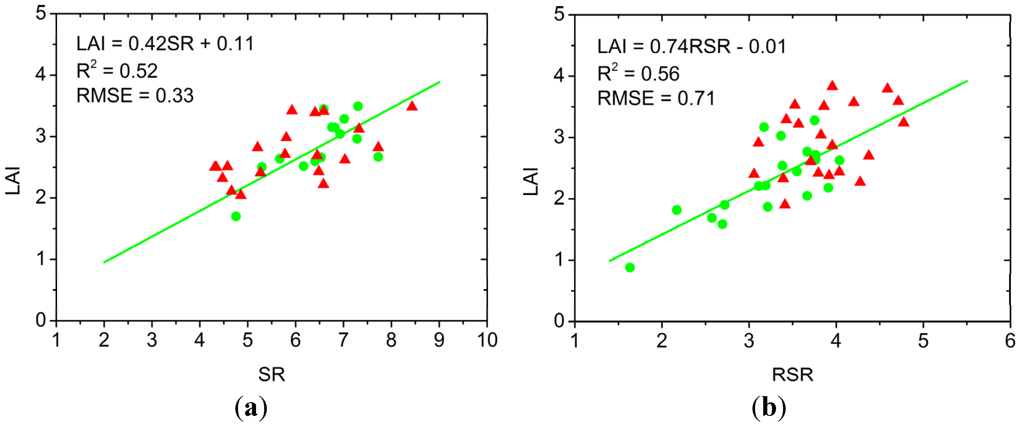
3.2.3. Development of LAI Reference Maps

We generated two LAI reference maps as “ground truth” in FEA and AREA. An empirical regression modeling approach was used to derive the transfer functions and to relate the field measurements to the vegetation index (VI) calculated from the corresponding synchronous fine-resolution satellite data (ETM + in FEA and ASTER in AREA). Three VIs were tested: Normalized Difference Vegetation Index (NDVI) [63], the simple ratio (SR) [64] and the reduced simple ratio (RSR) [65]. Regression analysis was performed separately for each image and VI. The regression model that provided the best linear relationship was chosen to generate a fine-resolution LAI map. The accuracy and robustness of the statistical models decreases when the size of the calibration database is limited [14]. Therefore, all of the in situ measurements (19 and 14 plots in FEA and AREA, respectively) were used to calibrate the regression lines to ensure their accuracy. The best linear regression equations to generate fine-resolution LAI maps were provided by SR in AREA and by RSR in FEA, with R²/RMSE equal to 0.52/0.33 and 0.56/0.71, respectively (Figure 2). Note that these linear relationships may not well be statistically significant. The performance of the regression lines is subject to the limited number and representativeness of the in situ measurements: there are only 19 and 14 measurements in FEA and AREA, respectively, and the values of LAI concentrate between two and 3.5.

Figure 2. The regression lines between VI and LAI in AREA (a) and FEA (b). The dots indicate the measurements described in Section 3.2.1 and were used to fit the regression lines. The triangles indicate the independent validation samples collected in different field campaigns in the same study area.

Figure 2. The regression lines between VI and LAI in AREA (a) and FEA (b). The dots indicate the measurements described in Section 3.2.1 and were used to fit the regression lines. The triangles indicate the independent validation samples collected in different field campaigns in the same study area.

To verify the accuracy of the regression lines, additional in situ LAI measurements collected on 11 August and 20 September 2012 in AREA and 12 to 15 July 2012 in FEA served as an independent validation dataset. The RMSEs calculated from the validation dataset are 0.55 and 0.79 in AREA and FEA, and the accuracy is acceptable considering the variation of the LAI-VI relationship over time [16]. However, more accurate measurements are required to obtain more statistically-sound results in future studies.

The established regression equations were applied to ASTER and ETM+ images and derived two fine-resolution LAI maps for the AREA and FEA sub-regions, respectively. Finally, the two fine-resolution LAI maps were aggregated to 500-m resolution and serve as reference LAI maps to assess the accuracy of the LAI maps retrieved by different RT models.

3.3. Synthetic Test Datasets

The SAIL and four-scale models were used to simulate reflectances with input variables varying within their respective definition intervals. The structural parameters of the SAIL (Table 2) and four-scale (Table 3) models were set according to a priori information gathered from the two field campaigns and other studies working within the same study area [66].

Table 2. Distribution of the canopy structure parameters of the scattering from arbitrarily inclined leaves (SAIL) model used to generate the training dataset.

Variable	Min	Mean	Max	Std	Distribution law	n class
LAI (m2/m2)	0	3.5	7	—	Uniform	7
ALA (°)	45	50	55	5	Truncated Gauss	4
H	0.3	0.4	0.5	0.1	Truncated Gauss	2

Table 2. Distribution of the canopy structure parameters of the scattering from arbitrarily inclined leaves (SAIL) model used to generate the training dataset.

Variable	Min	Mean	Max	Std	Distribution law	n class
LAI (m2/m2)	0	3.5	7	—	Uniform	7
ALA (°)	45	50	55	5	Truncated Gauss	4
H	0.3	0.4	0.5	0.1	Truncated Gauss	2

Table 3. Distribution of the canopy structure parameters of the four-scale model used to generate the training dataset.

	Variable	Min	Mean	Max	Std	Distribution law	n Class
site parameter	LAI (m2/m2)	0	3.5	7	—	Uniform	7
	Qz (ha)	1	1	1	0	Dirac delta	1
	Td (/ha)	1000	1250	1500	200	Truncated Gauss	1
	m2	5	5	5	—	Dirac delta	1
tree architecture parameters	r (m)	2	3	4	1	Truncated Gauss	4
	ha (m)	1	1	1	—	Dirac delta	1
	hb (m)	3.5	6.7	10	3	Truncated Gauss	4
	α (°)	13	13	13	—	Dirac delta	1
	γE	1.4	1.4	1.4	—	Dirac delta	1
	ΩE	0.65	0.65	0.65	—	Dirac delta	1
	Ws (m)	0.035	0.035	0.035	—	Dirac delta	1
	LIAD	spherical					1

Table 3. Distribution of the canopy structure parameters of the four-scale model used to generate the training dataset.

	Variable	Min	Mean	Max	Std	Distribution law	n Class
site parameter	LAI (m2/m2)	0	3.5	7	—	Uniform	7
	Qz (ha)	1	1	1	0	Dirac delta	1
	Td (/ha)	1000	1250	1500	200	Truncated Gauss	1
	m2	5	5	5	—	Dirac delta	1
tree architecture parameters	r (m)	2	3	4	1	Truncated Gauss	4
	ha (m)	1	1	1	—	Dirac delta	1
	hb (m)	3.5	6.7	10	3	Truncated Gauss	4
	α (°)	13	13	13	—	Dirac delta	1
	γE	1.4	1.4	1.4	—	Dirac delta	1
	ΩE	0.65	0.65	0.65	—	Dirac delta	1
	Ws (m)	0.035	0.035	0.035	—	Dirac delta	1
	LIAD	spherical					1

The optical properties of the leaves required by the two RT models were supplied by PROSPECT-4 [67] as a function of the mesophyll structure parameter (N), chlorophyll (C_ab), dry matter (C_dm), equivalent water thickness (C_w) and brown pigment (C_bp) contents. The distribution of values for each variable was specified based on the recommendation of [4] (Table 4), which is assumed to be globally representative. The soil reflectance was set as the mean of the measured soil spectrum during the two field campaigns (0.19 and 0.25 in the red and near-infrared bands, respectively). The specification of soil reflectance as a constant rather than a variable would not bring much uncertainty, considering the dense vegetation cover in our study area (the values of most LAI are greater than one in our study area). In addition, the Sun-target-sensor geometry was extracted from the MOD09GA data covering the study areas.

Table 4. Distribution of the input variables of the PROSPECT-4 model used to generate leaf reflectance and transmittance.

Variable	Min	Mean	Max	Std	Distribution law	n Class
N	1	1.5	2.5	1	Truncated Gauss	4
Cab (μg/cm)	20	45	90	30	Truncated Gauss	4
Cdm (g/cm)	0.002	0.0075	0.02	0.0075	Truncated Gauss	4
Cw (cm)	0.55	0.75	0.95	0.1	Truncated Gauss	4
Cbp	0	0	1.5	0.2	Truncated Gauss	4

Table 4. Distribution of the input variables of the PROSPECT-4 model used to generate leaf reflectance and transmittance.

Variable	Min	Mean	Max	Std	Distribution law	n Class
N	1	1.5	2.5	1	Truncated Gauss	4
Cab (μg/cm)	20	45	90	30	Truncated Gauss	4
Cdm (g/cm)	0.002	0.0075	0.02	0.0075	Truncated Gauss	4
Cw (cm)	0.55	0.75	0.95	0.1	Truncated Gauss	4
Cbp	0	0	1.5	0.2	Truncated Gauss	4

To sample the multi-dimensional parameter spaces of the SAIL and four-scale models representatively and efficiently, the sampling method proposed by [68] was adopted. In this sampling method, the definition interval of each variable was split into a given number of classes (see Table 2, Table 3 and Table 4). All combinations of classes were sampled only once. This allows for accounting for all of the interactions between variables, while having each variable sampled nearly randomly. For each combination of input variables, TOC reflectance was computed for each wavelength and then integrated according to the spectral response function of MODIS. A total of 57,344 and 114,688 cases were simulated for SAIL and the four-scale models, respectively. The number of simulations is defined by the trade-off between accuracy and computer resources. For LAI retrieval, more than 1000 simulations are enough to train the NN [48].

Both datasets simulated by the SAIL and four-scale models were randomly split into three subsets [48]: the first one made of half the cases was used to train the NNs; the second one made of one fourth the cases was used to avoid the over-fitness during the learning process; and the rest of the cases served as the synthetic test dataset.

4. Results and Discussion

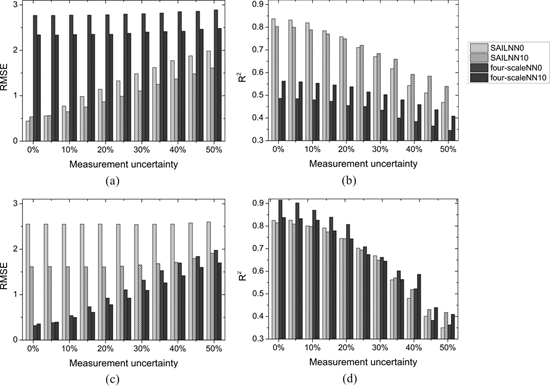
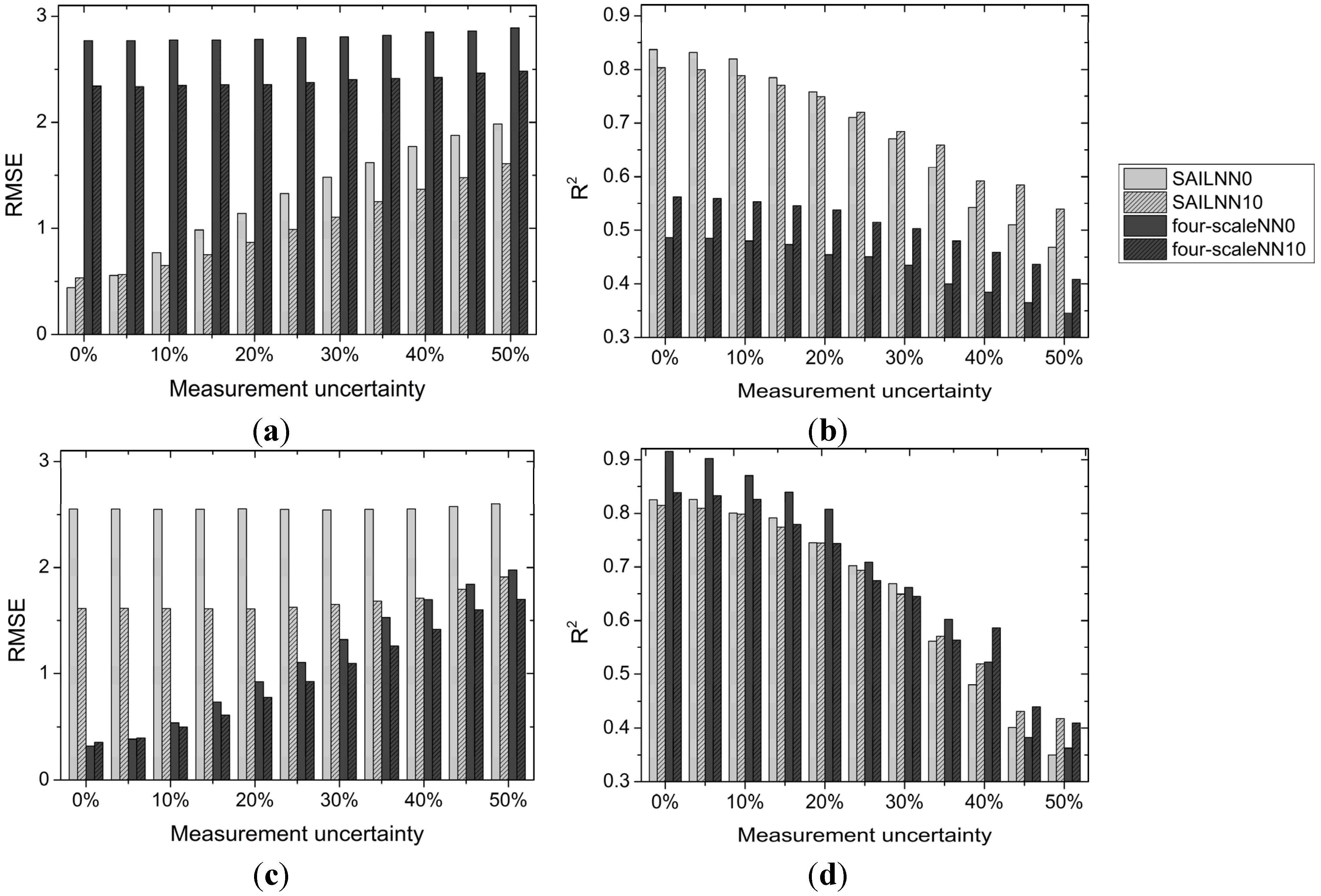
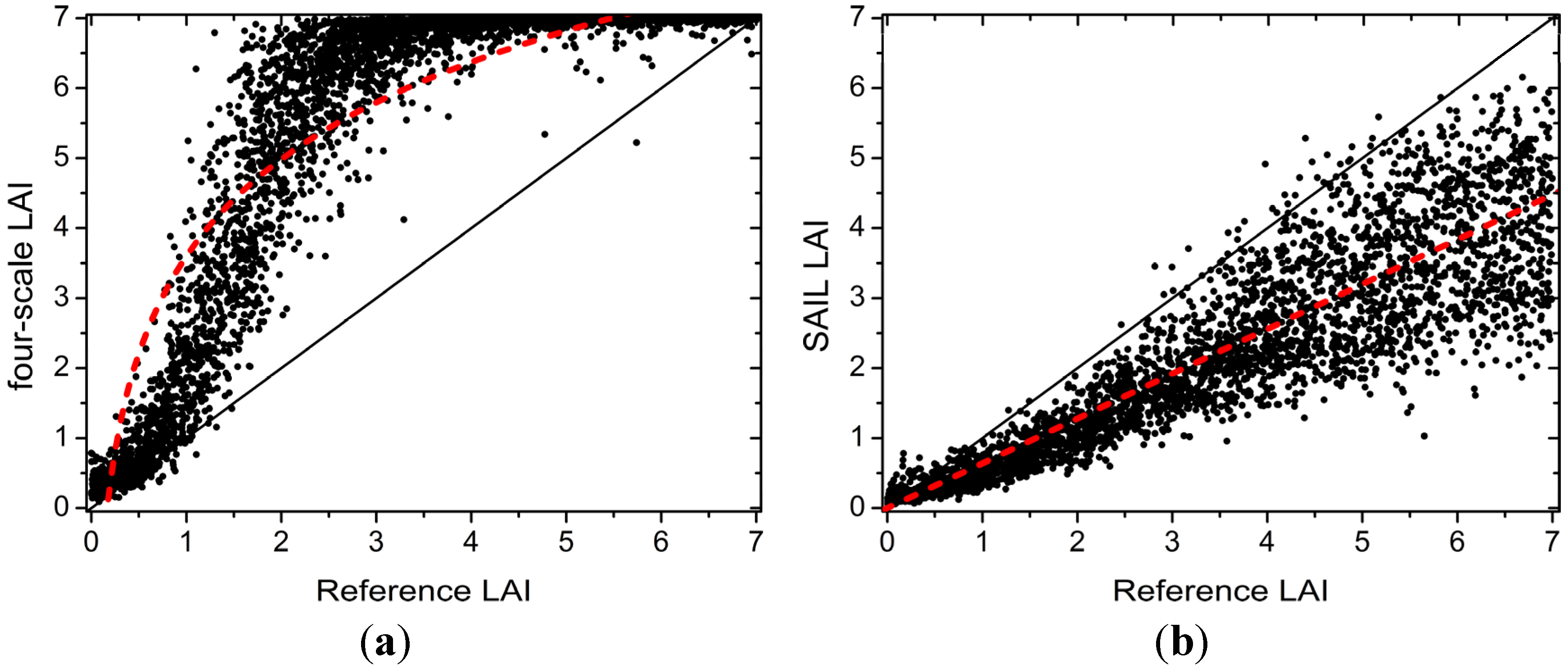
4.1. Robustness to Uncertainty in Reflectances

The robustness of retrieval methods to uncertainty in reflectances is important, particularly in the context of the concurrent use of multi-sensor data. This was investigated by adding white Gaussian noise (ranging from zero, for noise-free reflectances, to 50%, for very noisy reflectances) to the simulated reflectances in the synthetic test datasets. Correspondingly, adding white Gaussian noise to the inversion methods (e.g., LUT and NN) is a common strategy to account for the measurement uncertainty. However, there is no consolidated criterion to specify the variance of the white Gaussian noise. Adding too little noise in the inversion methods means a high accuracy for noise-free reflectances, but it may be sensitive to potential uncertainty embed in reflectances. On the other hand, adding too much noise reduces the retrieval accuracy. In this study, we established two counterparts for SAILNN and four-scaleNN by adding 10% Gaussian noise to the corresponding training datasets, which are denoted as SAILNN10 and four-scaleNN10, respectively. The uncertainty level (10%) was determined by gradually increasing the values from 2% to 20% in 2% increments to get a good compromise between accuracy and robustness. The four NNs (SAILNN0, SAILNN10, four-scaleNN0 and four-scaleNN10) were applied to the synthetic test datasets contaminated by different levels of Gaussian noise (ranging from 0% to 50%).

The results derived from the synthetic test datasets from both SAIL (Figure 3a,c) and four-scale model (Figure 3b,d) simulations show the same trend. The measurement uncertainty degrades the retrieval accuracy, as manifested by the increasing RMSE and the decreasing R². It is difficult to quantify the real measurement uncertainty, but it is assumed to be around 20% [69]. This value may be higher when considering the differences between sensor-specific characteristics in the context of the concurrent use of multi-sensor data. Therefore, the quality and consistency of the inputs of retrieval algorithms should be further confirmed. When appropriate RT models are used, i.e., using the SAIL model for the SAIL test dataset and using the four-scale model for the four-scale synthetic test dataset, the NNs that contain noise (SAILNN10 and four-scaleNN10) get a lower accuracy compared with the original NNs (SAILNN0 and four-scaleNN0) for the unavailable pure measurements (with the abscissa values equal to 0% in Figure 3), but they were more robust to the measurement uncertainties. Therefore, adding a reasonable amount of noise to the training dataset can be seen as a regularization method [48,70]. The results in Section 4.2 and Section 4.3 are all derived from these two noisy NNs.

Figure 3. RMSE and R² between the estimated and actual LAI values over the SAIL (a,b) and four-scale (c,d) synthetic test datasets as a function of measurement uncertainty. The SAIL and four-scale synthetic test datasets were simulated by the SAIL and four-scale models, respectively. The four bars for a specific uncertainty level represent the original SAIL and four-scaleNN without noise (SAILNN0 and four-scaleNN0), and the SAIL and four-scaleNN trained using 10% Gaussian white noisy training database (SAILNN10 and four-scaleNN10). Measurement uncertainty represents the corresponding level of Gaussian noise added to the synthetic test dataset.

Figure 3. RMSE and R² between the estimated and actual LAI values over the SAIL (a,b) and four-scale (c,d) synthetic test datasets as a function of measurement uncertainty. The SAIL and four-scale synthetic test datasets were simulated by the SAIL and four-scale models, respectively. The four bars for a specific uncertainty level represent the original SAIL and four-scaleNN without noise (SAILNN0 and four-scaleNN0), and the SAIL and four-scaleNN trained using 10% Gaussian white noisy training database (SAILNN10 and four-scaleNN10). Measurement uncertainty represents the corresponding level of Gaussian noise added to the synthetic test dataset.

It also can be seen from Figure 3 that model selection has a great impact on LAI retrieval. When an unsuitable RT model is used, the value of RMSE is unacceptably high (Figure 3a,b), and these values are stable as measurement uncertainty increases: the RS observations can hardly be converted to useful information for LAI retrieval without an appropriate RT model. Using SAILNN on the four-scale synthetic test dataset obtained better results than using four-scaleNN on the SAIL synthetic test dataset. As for the four-scale synthetic test dataset, the retrieved LAI from SAILNN is linearly well related to the actual LAI (SAILNN gets comparable R² than four-scaleNN, as shown in Figure 3d), though they differ in magnitude (Figure 3b). This implies that, in the context of LAI retrieval, using a simple RT model for a complex scenario is more appropriate than the opposite case. Although a complex model can always be parameterized to represent the simple model’s output, its complexity in canopy structure representation limits the generalization capability and results in poor retrieval accuracy without sufficient a priori information.

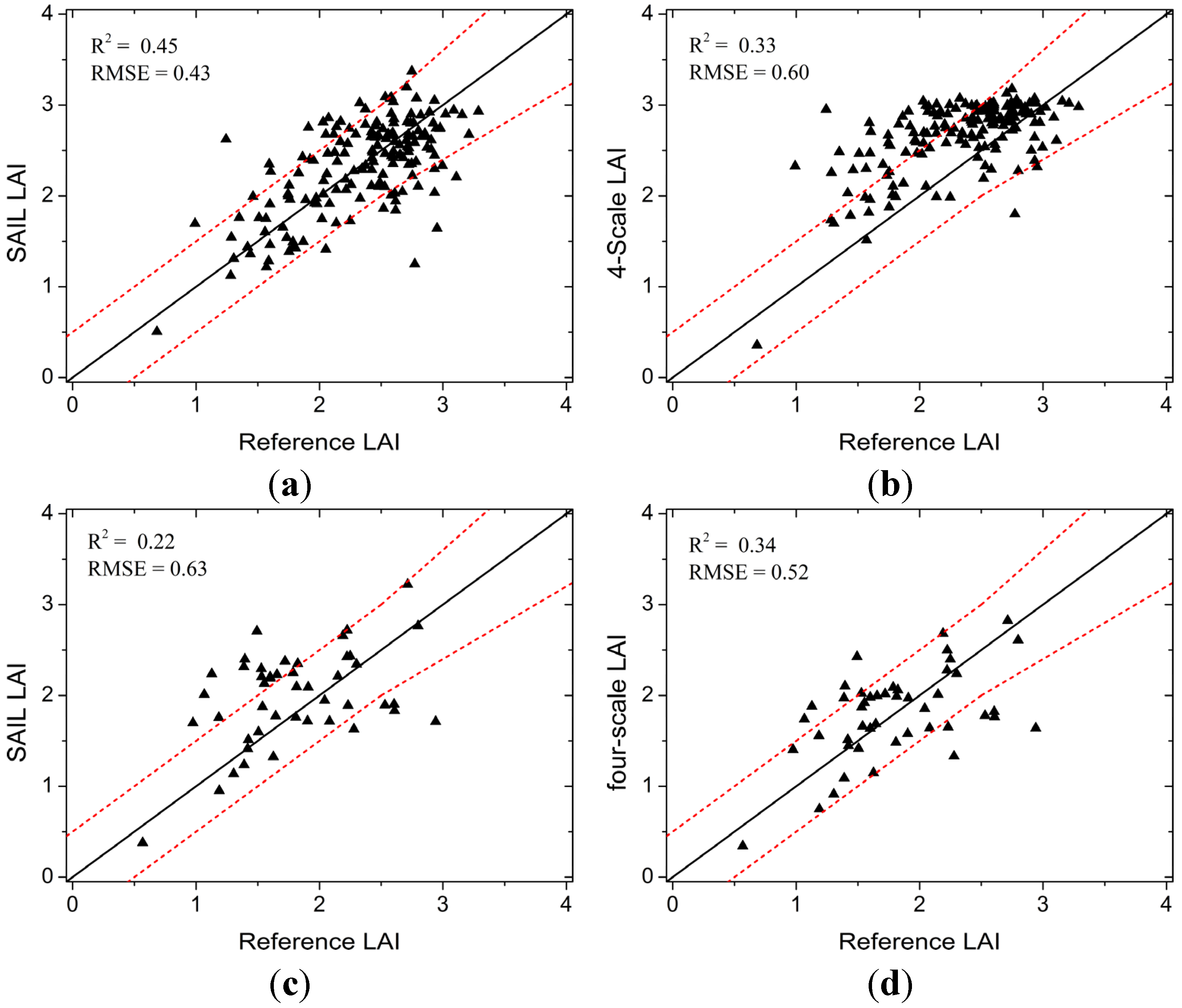
4.2. Impact of RT Model Selection on Retrieval Accuracy

The scatter plots of the estimated and actual values of LAI over the two synthetic test datasets are shown in Figure 4a,b. In these two figures, the estimated LAI was obtained by interchangeably using the two NNs, i.e., using four-scaleNN to invert the SAIL test dataset (Figure 4a) and using SAILNN to invert the four-scale test dataset (Figure 4b). The former case shows an obvious overestimation with the RMSE equal to 2.3. The relationship between the reference and retrieved LAI can be well stated with a logarithmic function (y = 2lnx + 3.6) with R² = 0.8, but the parameters in the fitted function have no apparent physical meanings. When LAI is greater than 2.5, the four-scaleNN becomes less sensitive to the change in LAI; this is because in this case, the crown is saturated with foliage. A further increase in LAI has a negligible influence on the radiative transfer within the crown. In the latter case, the reference and retrieved LAI is highly linearly correlated (y = 0.64x), with R² = 0.82. The slope of the zero-intercepted fitted line is comparable to the clumping index entered to the four-scale simulations (0.65, Ω_E in Table 3). This result proves that with an increasing number of accurate clumping index maps [71,72], the LAI of a complex scenario (e.g., forests and savanna) can be retrieved using a 1D RT model and then post-processed with the clumping index to obtain the final result.

Figure 4. Scatter plots of the estimated and actual values of LAI. Using four-scaleNN to invert the SAIL test dataset (a) and using SAILNN to invert the four-scale test dataset (b). The dashed lines are the regression lines between the estimated and actual LAI.

Figure 4. Scatter plots of the estimated and actual values of LAI. Using four-scaleNN to invert the SAIL test dataset (a) and using SAILNN to invert the four-scale test dataset (b). The dashed lines are the regression lines between the estimated and actual LAI.

To assess the influence of RT model selection more realistic, LAI maps, in our study area, retrieved by the SAIL and four-scale models, were compared with the corresponding 500-m reference maps. This inter-comparison was implemented over 3 × 3 pixel windows to minimize the uncertainty caused by geolocation errors and the difference in the point spread function [60]. Only windows with more than seven croplands or forests pixels were chosen to reduce the influence of surface heterogeneity. The median of the LAI values within each window was used for the inter-comparison. The results are presented in Figure 5.

Figure 5. Comparison between SAIL LAI (a) and four-scale LAI (b) in croplands and SAIL LAI (c) and four-scale LAI (d) in forests with the corresponding reference LAI. The solid lines represent the 1:1 lines, and the dotted lines represent the accuracy boundaries (max (0.5, 20%)) specified by the Global Climate Observation System (GCOS).

Figure 5. Comparison between SAIL LAI (a) and four-scale LAI (b) in croplands and SAIL LAI (c) and four-scale LAI (d) in forests with the corresponding reference LAI. The solid lines represent the 1:1 lines, and the dotted lines represent the accuracy boundaries (max (0.5, 20%)) specified by the Global Climate Observation System (GCOS).

In the cropland-dominated AREA sub-region (Figure 5a,b), the SAIL LAI shows much better agreement with the reference LAI (R² = 0.45 and RMSE = 0.43) than four-scale LAI (R² =0.33 and RMSE = 0.60). An obvious overestimation is observed for the four-scale LAI. This phenomenon is mainly caused by the canopy structure representation of the four-scale model, which assumes that the canopy is composed of several discrete crowns. This representation is entirely unrealistic for croplands.

In the forest-dominated FEA sub-region, the SAILNN and four-scaleNN produce similar results, with four-scaleNN performing slightly better (Figure 5c,d). Theoretically, the canopy structure representation of the four-scale model is far more realistic than the SAIL model for forests. However, the high fidelity in the canopy structure representation does not necessarily imply a high inverse accuracy of the same magnitude. This is partly because the extensive parameterization of the four-scale model requires so many inputs, which are difficult to specify, that its potential to retrieve LAI is constrained by the lack of information. Another reason explaining this phenomenon is that the definition of LAI in the experimental test dataset corresponds to effective LAI. The assumption that underlies this definition is similar to that for the SAIL model: the foliage is randomly distributed in the canopy [39].

Although the retrieval accuracy may be not satisfactorily high, it proves the importance of canopy structure representation in RT models. If an unsuitable RT model, which is unrealistic for canopy structure representation, is used, then the RMSE will increase from 0.43 to 0.60 in croplands and from 0.52 to 0.63 in forests. Therefore, physically-based retrieval algorithms should embed more than one RT model to account for the variations in structural attributes among different vegetation types (see Table 1).

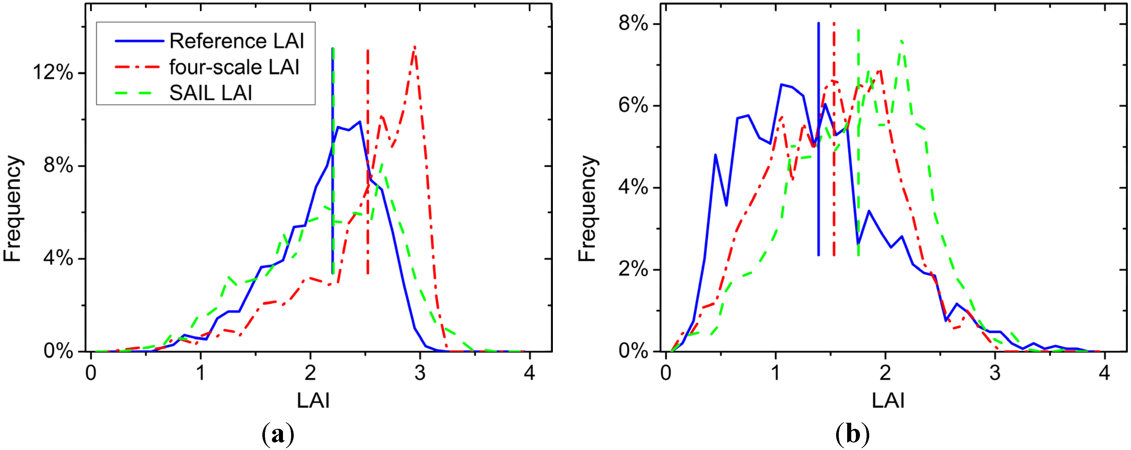
4.3. Impact on LAI Spatial Variability Quantification

The quantification of the LAI spatial variability is very important for forcing regional land surface process models. Inaccurate quantification will cause scale error [73]. Figure 6 displays the distribution of the LAI values for each LAI map in AREA (Figure 6a) and FEA (Figure 6b).

Figure 6. Distribution of the LAI values for each LAI map in AREA (a) and FEA (b). The solid, dashed and dash-doted vertical bars identify the locations of the mean values for the reference, SAIL and four-scale LAI, respectively.

Figure 6. Distribution of the LAI values for each LAI map in AREA (a) and FEA (b). The solid, dashed and dash-doted vertical bars identify the locations of the mean values for the reference, SAIL and four-scale LAI, respectively.

In AREA, the reference LAI presents an approximate normal distribution. The distribution pattern of the SAIL LAI is very similar to that of the reference LAI, with nearly identical mean values (2.2). However, the four-scale LAI shows an unrealistic positive skew and overestimation, with a very high peak at around 3.0 and mean at around 2.5. For FEA, all of the three LAI maps display turbulent distributions. The SAIL LAI histogram has a similar shape to the four-scale LAI histogram, but with a shift to high values. A discrepancy between the two retrieved LAI and reference LAI is observed, but the four-scale LAI is more similar to the reference LAI, as revealed by its mean LAI value (1.5), which is more similar to that of the reference LAI (1.4) than the SAIL LAI (1.8).

To quantitatively analyze the impact of RT model selection on the regional LAI spatial variability characterization, we calculated the K-L divergence (Equation (1)). In AREA, D_KL(LAI_ref||LAI_SAIL) and D_KL(LAI_ref||LAI_four-scale) are 0.18 and 0.61, respectively. In FEA, these values are 0.43 and 0.17. Therefore, when retrieving LAI, the croplands and forests respectively prefer SAIL and four-scale models in terms of information fidelity. However, using the SAIL model in forests results in less information loss than using the four-scale model in croplands (0.43 vs. 0.61 for K-L divergence).

Therefore, the effect of RT model selection is not only related to the bidirectional reflectance distribution function (BRDF) fitting capacity, but it is also subject to the availability of a priori information on RT model parameters. Generally, a complex RT model requires more a priori information to avoid unreasonable variable combinations and to constrain the solution to a sufficiently small interval in parameter space. Therefore, 3D RT models may not be appropriate in the case of a priori information insufficiency. Note that the complexity in canopy structure and the high sensitivity of RT models to a priori information can partly explain the lower accuracy of LAI retrieved over forests than over other land cover types. In reality, simplicity alone can be seen as a criterion for judging models in the context of LAI retrieval, and RT model selection is carried out by trading off goodness-of-fit and simplicity.

Therefore, when a priori information is sufficient, RT models that can realistically characterize structural properties are preferable (see Table 1). Without sufficient a priori information, the 1D RT models that are simpler in terms of structural parameterization would perform better than 3D models. Furthermore, the a priori information is preferably expressed in an explicitly spatial manner rather than by distribution/co-distributions of RT model parameters. The explicitly spatial manner may be benefited from the availability of new biophysical parameters retrieved from RS, e.g., clumping index and tree height. With the emergence of such biophysical products, the advantage of 3D over 1D RT models in complex scenarios will be further explored in the future.

5. Conclusions

The major aim of this study is to assess the impact of RT model selection on LAI retrieval. In general, the fidelity in canopy structure representation of RT models has remarkable implications on LAI retrieval. If an unsuitable RT model, which is unrealistic in terms of structure representation, is used, the RMSE will increase from 0.43 to 0.60 in croplands and from 0.52 to 0.63 in forests. Nevertheless, the structural fidelity is not the only determinant in RT model selection, and the potential of an RT model to retrieve LAI is also limited by the availability of a priori information. 3D RT models rely more on a priori information, resulting in poorer generalization capacity. The problem of RT model selection is finding an appropriate compromise between goodness-of-fit and simplicity. Therefore, 1D RT models are recommended when a priori information is insufficient, even for forests, and the retrieved result can be post-processed using freely available clumping index products. As the emergence of some new biophysical products, e.g., clumping index and tree height, the advantage of 3D over 1D RT models in complex scenarios will be further explored in the future.

To establish an operational retrieval approach suitable for LAI inversion at the global scale, the analysis in this paper should be expanded. Firstly, only the most widely-used red and near-infrared bands were involved in the inversion approach. It may be valuable to assess the feasibility of other bands to improve the LAI accuracy. Secondly, only two types of test datasets (representing the structural properties of croplands and needle leaf forests) and two RT models (SAIL and four-scale) were tested. To refine and confirm the results, more models should be assessed by using more representative test datasets. Thirdly, input noise and inconsistency degrade the retrieval accuracy and restrain the advantage of appropriable RT models, which have highly realistic canopy structure representation. Therefore, an improved pre-processing algorithm of reflectance is required particularly when multi-sensor data are concurrently used. Finally, the architecture of NN was established by a trial-and-error approach that may impact the final robustness of the trained NN. Other more advanced regression methods are needed to improve our study, and the use of the Automated Radiative Transfer Models Operator (ARTMO) toolbox [74,75] will greatly facilitate future improvements.

References

1. Sellers, P.; Dickinson, R.; Randall, D.; Betts, A.; Hall, F.; Berry, J.; Collatz, G.; Denning, A.; Mooney, H.; Nobre, C. Modeling the exchanges of energy, water, and carbon between continents and the atmosphere. Science 1997, 275, 502–509. [Google Scholar] [CrossRef] [PubMed]
2. Myneni, R.; Hoffman, S.; Knyazikhin, Y.; Privette, J.; Glassy, J.; Tian, Y.; Wang, Y.; Song, X.; Zhang, Y.; Smith, G. Global products of vegetation leaf area and fraction absorbed PAR from year one of MODIS data. Remote Sens. Environ. 2002, 83, 214–231. [Google Scholar] [CrossRef]
3. Baret, F.; Weiss, M.; Lacaze, R.; Camacho, F.; Makhmara, H.; Pacholcyzk, P.; Smets, B. GEOV1: LAI and FAPAR essential climate variables and FCOVER global time series capitalizing over existing products. Part1: Principles of development and production. Remote Sens. Environ. 2013, 137, 299–309. [Google Scholar] [CrossRef]
4. Baret, F.; Hagolle, O.; Geiger, B.; Bicheron, P.; Miras, B.; Huc, M.; Berthelot, B.; Niño, F.; Weiss, M.; Samain, O. LAI, fAPAR and fCover CYCLOPES global products derived from VEGETATION: Part 1: Principles of the algorithm. Remote Sens. Environ. 2007, 110, 275–286. [Google Scholar] [CrossRef] [Green Version]
5. Pinty, B.; Andredakis, I.; Clerici, M.; Kaminski, T.; Taberner, M.; Verstraete, M.; Gobron, N.; Plummer, S.; Widlowski, J.L. Exploiting the MODIS albedos with the Two-stream Inversion Package (JRC-TIP): 1. Effective leaf area index, vegetation, and soil properties. J. Geophys. Res. 2011, 116, D09105. [Google Scholar]
6. Xiao, Z.; Liang, S.; Wang, J.; Chen, P.; Yin, X.; Zhang, L.; Song, J. Use of general regression neural networks for generating the GLASS leaf area index product from time-series MODIS surface reflectance. IEEE Trans. Geosci. Remote Sens. 2014, 52, 209–223. [Google Scholar] [CrossRef]
7. Deng, F.; Chen, M.; Plummer, S.; Pisek, J. Algorithm for global leaf area index retrieval using satellite imagery. IEEE Trans. Geosci. Remote Sens. 2006, 44, 2219–2229. [Google Scholar] [CrossRef]
8. Fang, H.; Wei, S.; Liang, S. Validation of MODIS and CYCLOPES LAI products using global field measurement data. Remote Sens. Environ. 2012, 119, 43–54. [Google Scholar] [CrossRef]
9. Garrigues, S.; Lacaze, R.; Baret, F.; Morisette, J.; Weiss, M.; Nickeson, J.; Fernandes, R.; Plummer, S.; Shabanov, N.; Myneni, R. Validation and intercomparison of global Leaf Area Index products derived from remote sensing data. J. Geophys. Res. 2008, 113, G02028. [Google Scholar]
10. Garrigues, S.; Allard, D.; Baret, F.; Weiss, M. Influence of landscape spatial heterogeneity on the non-linear estimation of leaf area index from moderate spatial resolution remote sensing data. Remote Sens. Environ. 2006, 105, 286–298. [Google Scholar] [CrossRef]
11. Yin, G.; Li, J.; Liu, Q.; Li, L.; Zeng, Y.; Xu, B.; Yang, L.; Zhao, J. Improving Leaf Area Index Retrieval Over Heterogeneous Surface by Integrating Textural and Contextual Information: A Case Study in the Heihe River Basin. IEEE Geosci. Remote Sens. Lett. 2015, 12, 359–363. [Google Scholar] [CrossRef]
12. Verger, A.; Baret, F.; Weiss, M. A multisensor fusion approach to improve LAI time series. Remote Sens. Environ. 2011, 115, 2460–2470. [Google Scholar] [CrossRef]
13. Widlowski, J.L.; Pinty, B.; Lopatka, M.; Atzberger, C.; Buzica, D.; Chelle, M.; Disney, M.; Gastellu-Etchegorry, J.P.; Gerboles, M.; Gobron, N.; et al. The fourth radiation transfer model intercomparison (RAMI-IV): Proficiency testing of canopy reflectance models with ISO-13528. J. Geophys. Res. 2013, 118, 6869–6890. [Google Scholar]
14. Atzberger, C.; Darvishzadeh, R.; Immitzer, M.; Schlerf, M.; Skidmore, A.; le Maire, G. Comparative analysis of different retrieval methods for mapping grassland leaf area index using airborne imaging spectroscopy. Int. J. Appl. Earth Obs. Geoinf. 2015. [Google Scholar] [CrossRef]
15. Baret, F.; Buis, S. Estimating Canopy Characteristics from Remote Sensing Observations: Review of Methods and Associated Problems. In Advances in Land Remote Sensing; Springer: Berlin, Germany, 2008; pp. 173–201. [Google Scholar]
16. Tillack, A.; Clasen, A.; Kleinschmit, B.; Förster, M. Estimation of the seasonal leaf area index in an alluvial forest using high-resolution satellite-based vegetation indices. Remote Sens. Environ. 2014, 141, 52–63. [Google Scholar] [CrossRef]
17. Viña, A.; Gitelson, A.A.; Nguy-Robertson, A.L.; Peng, Y. Comparison of different vegetation indices for the remote assessment of green leaf area index of crops. Remote Sens. Environ. 2011, 115, 3468–3478. [Google Scholar] [CrossRef]
18. Strahler, A.H. Vegetation canopy reflectance modeling—Recent developments and remote sensing perspectives. Remote Sens. Rev. 1997, 15, 179–194. [Google Scholar] [CrossRef]
19. Jacquemoud, S.; Bacour, C.; Poilve, H.; Frangi, J.-P. Comparison of four radiative transfer models to simulate plant canopies reflectance: Direct and inverse mode. Remote Sens. Environ. 2000, 74, 471–481. [Google Scholar] [CrossRef]
20. Fang, H.; Liang, S. A hybrid inversion method for mapping leaf area index from MODIS data: Experiments and application to broadleaf and needleleaf canopies. Remote Sens. Environ. 2005, 94, 405–424. [Google Scholar] [CrossRef]
21. Qi, J.; Kerr, Y.; Moran, M.; Weltz, M.; Huete, A.; Sorooshian, S.; Bryant, R. Leaf area index estimates using remotely sensed data and BRDF models in a semiarid region. Remote Sens. Environ. 2000, 73, 18–30. [Google Scholar] [CrossRef]
22. Verrelst, J.; Alonso, L.; Caicedo, J.P.R.; Moreno, J.; Camps-Valls, G. Gaussian process retrieval of chlorophyll content from imaging spectroscopy data. IEEE J. Sel. Top. Appl. Earth Obs. Remote Sens. 2013, 6, 867–874. [Google Scholar] [CrossRef]
23. Verrelst, J.; Alonso, L.; Camps-Valls, G.; Delegido, J.; Moreno, J. Retrieval of vegetation biophysical parameters using Gaussian process techniques. IEEE Trans. Geosci. Remote Sens. 2012, 50, 1832–1843. [Google Scholar] [CrossRef]
24. Qu, Y.; Han, W.; Ma, M. Retrieval of a Temporal high-resolution Leaf Area Index (LAI) by combining MODIS LAI and ASTER reflectance data. Remote Sensing. 2015, 7, 195–210. [Google Scholar] [CrossRef]
25. Qu, Y.; Zhang, Y.; Wang, J. A dynamic Bayesian network data fusion algorithm for estimating leaf area index using time-series data from in situ measurement to remote sensing observations. Int. J. Remote Sens. 2012, 33, 1106–1125. [Google Scholar] [CrossRef]
26. Lauvernet, C.; Baret, F.; Hascoët, L.; Buis, S.; Le Dimet, F.-X. Multitemporal-patch ensemble inversion of coupled surface–atmosphere radiative transfer models for land surface characterization. Remote Sens. Environ. 2008, 112, 851–861. [Google Scholar] [CrossRef]
27. Combal, B.; Baret, F.; Weiss, M.; Trubuil, A.; Mace, D.; Pragnere, A.; Myneni, R.; Knyazikhin, Y.; Wang, L. Retrieval of canopy biophysical variables from bidirectional reflectance: Using prior information to solve the ill-posed inverse problem. Remote Sens. Environ. 2003, 84, 1–15. [Google Scholar] [CrossRef]
28. Atzberger, C. Object-based retrieval of biophysical canopy variables using artificial neural nets and radiative transfer models. Remote Sens. Environ. 2004, 93, 53–67. [Google Scholar] [CrossRef]
29. Atzberger, C.; Richter, K. Spatially constrained inversion of radiative transfer models for improved LAI mapping from future Sentinel-2 imagery. Remote Sens. Environ. 2012, 120, 208–218. [Google Scholar] [CrossRef]
30. Houborg, R.; Soegaard, H.; Boegh, E. Combining vegetation index and model inversion methods for the extraction of key vegetation biophysical parameters using Terra and Aqua MODIS reflectance data. Remote Sens. Environ. 2007, 106, 39–58. [Google Scholar] [CrossRef]
31. Houborg, R.; McCabe, M.; Cescatti, A.; Gao, F.; Schull, M.; Gitelson, A. Joint leaf chlorophyll content and leaf area index retrieval from Landsat data using a regularized model inversion system (REGFLEC). Remote Sens. Environ. 2015. [Google Scholar]
32. Widlowski, J.-L.; Côté, J.-F.; Béland, M. Abstract tree crowns in 3D radiative transfer models: Impact on simulated open-canopy reflectances. Remote Sens. Environ. 2014, 142, 155–175. [Google Scholar] [CrossRef]
33. Yao, Y.; Liu, Q.; Liu, Q.; Li, X. LAI retrieval and uncertainty evaluations for typical row-planted crops at different growth stages. Remote Sens. Environ. 2008, 112, 94–106. [Google Scholar] [CrossRef]
34. Widlowski, J.-L.; Pinty, B.; Lavergne, T.; Verstraete, M.M.; Gobron, N. Using 1-D models to interpret the reflectance anisotropy of 3-D canopy targets: Issues and caveats. IEEE Trans. Geosci. Remote Sens. 2005, 43, 2008–2017. [Google Scholar] [CrossRef]
35. Chen, J.; Black, T. Foliage area and architecture of plant canopies from sunfleck size distributions. Agric. For. Meteorol. 1992, 60, 249–266. [Google Scholar] [CrossRef]
36. Kucharik, C.J.; Norman, J.M.; Gower, S.T. Characterization of radiation regimes in nonrandom forest canopies: Theory, measurements, and a simplified modeling approach. Tree Physiol. 1999, 19, 695–706. [Google Scholar] [CrossRef] [PubMed]
37. Huang, D.; Knyazikhin, Y.; Wang, W.; Deering, D.W.; Stenberg, P.; Shabanov, N.; Tan, B.; Myneni, R.B. Stochastic transport theory for investigating the three-dimensional canopy structure from space measurements. Remote Sens. Environ. 2008, 112, 35–50. [Google Scholar] [CrossRef]
38. Chen, J.M.; Leblanc, S.G. A four-scale bidirectional reflectance model based on canopy architecture. IEEE Trans. Geosci. Remote Sens. 1997, 35, 1316–1337. [Google Scholar] [CrossRef]
39. Verhoef, W. Light scattering by leaf layers with application to canopy reflectance modeling: The SAIL model. Remote Sens. Environ. 1984, 16, 125–141. [Google Scholar] [CrossRef]
40. Pinty, B.; Gobron, N.; Widlowski, J.L.; Lavergne, T.; Verstraete, M. Synergy between 1-D and 3-D radiation transfer models to retrieve vegetation canopy properties from remote sensing data. J. Geophys. Res. 2004, 109. [Google Scholar] [CrossRef]
41. Pinty, B.; Lavergne, T.; Dickinson, R.; Widlowski, J.L.; Gobron, N.; Verstraete, M. Simplifying the interaction of land surfaces with radiation for relating remote sensing products to climate models. J. Geophys. Res. 2006, 111. [Google Scholar] [CrossRef]
42. Rautiainen, M.; Stenberg, P.; Nilson, T.; Kuusk, A. The effect of crown shape on the reflectance of coniferous stands. Remote Sens. Environ. 2004, 89, 41–52. [Google Scholar] [CrossRef]
43. Gastellu-Etchegorry, J.; Martin, E.; Gascon, F. DART: A 3D model for simulating satellite images and studying surface radiation budget. Int. J. Remote Sens. 2004, 25, 73–96. [Google Scholar] [CrossRef]
44. North, P. Three-dimensional forest light interaction model using a Monte Carlo method. IEEE Trans. Geosci. Remote Sens. 1996, 34, 946–956. [Google Scholar] [CrossRef]
45. Richter, K.; Atzberger, C.; Vuolo, F.; D'Urso, G. Evaluation of Sentinel-2 Spectral Sampling for Radiative Transfer Model Based LAI Estimation of Wheat, Sugar Beet, and Maize. IEEE J. Sel. Top. Appl. Earth Obs. Remote Sens. 2011, 4, 458–464. [Google Scholar] [CrossRef]
46. Myneni, R.B.; Ramakrishna, R.; Nemani, R.; Running, S.W. Estimation of global leaf area index and absorbed PAR using radiative transfer models. IEEE Trans. Geosci. Remote Sens. 1997, 35, 1380–1393. [Google Scholar] [CrossRef]
47. Duthoit, S.; Demarez, V.; Gastellu-Etchegorry, J.-P.; Martin, E.; Roujean, J.-L. Assessing the effects of the clumping phenomenon on BRDF of a maize crop based on 3D numerical scenes using DART model. Agric. For. Meteorol. 2008, 148, 1341–1352. [Google Scholar] [CrossRef]
48. Verger, A.; Baret, F.; Camacho, F. Optimal modalities for radiative transfer-neural network estimation of canopy biophysical characteristics: Evaluation over an agricultural area with CHRIS/PROBA observations. Remote Sens. Environ. 2011, 115, 415–426. [Google Scholar] [CrossRef]
49. Ngia, L.S.; Sjoberg, J. Efficient training of neural nets for nonlinear adaptive filtering using a recursive Levenberg-Marquardt algorithm. IEEE Trans. Signal Process. 2000, 48, 1915–1927. [Google Scholar] [CrossRef]
50. Hovi, A.; Korpela, I. Real and simulated waveform-recording LiDAR data in juvenile boreal forest vegetation. Remote Sens. Environ. 2014, 140, 665–678. [Google Scholar] [CrossRef]
51. Burnham, K.P.; Anderson, D.R. Model Selection and Multimodel Inference: A Practical Information-Theoretic Approach; Springer: Berlin, Germany, 2002. [Google Scholar]
52. Li, X.; Li, X.W.; Li, Z.Y.; Ma, M.G.; Wang, J.; Xiao, Q.; Liu, Q.; Che, T.; Chen, E.X.; Yan, G.J.; et al. Watershed Allied Telemetry Experimental Research. J. Geophys. Res. 2009, 114. [Google Scholar] [CrossRef]
53. Li, X.; Cheng, G.D.; Liu, S.M.; Xiao, Q.; Ma, M.G.; Jin, R.; Che, T.; Liu, Q.H.; Wang, W.Z.; Qi, Y.; et al. Heihe Watershed Allied Telemetry Experimental Research (HiWATER): Scientific Objectives and Experimental Design. Bull. Am. Meteorol. Soc. 2013, 94, 1145–1160. [Google Scholar] [CrossRef]
54. Data Management Center of The Heihe Plan. Available online: http://heihedata.org/ (accessed on 15 November 2014).
55. Pickett-Heaps, C.A.; Canadell, J.G.; Briggs, P.R.; Gobron, N.; Haverd, V.; Paget, M.J.; Pinty, B.; Raupach, M.R. Evaluation of six satellite-derived Fraction of Absorbed Photosynthetic Active Radiation (FAPAR) products across the Australian continent. Remote Sens. Environ. 2014, 140, 241–256. [Google Scholar] [CrossRef]
56. Wu, H.; Tang, B.-H.; Li, Z.-L. Impact of nonlinearity and discontinuity on the spatial scaling effects of the leaf area index retrieved from remotely sensed data. Int. J. Remote Sens. 2013, 34, 3503–3519. [Google Scholar] [CrossRef]
57. Claverie, M.; Vermote, E.F.; Weiss, M.; Baret, F.; Hagolle, O.; Demarez, V. Validation of coarse spatial resolution LAI and FAPAR time series over cropland in southwest France. Remote Sens. Environ. 2013, 139, 216–230. [Google Scholar] [CrossRef]
58. Chen, J.M. Optically-based methods for measuring seasonal variation of leaf area index in boreal conifer stands. Agric. For. Meteorol. 1996, 80, 135–163. [Google Scholar] [CrossRef]
59. Zeng, Y.L.; Li, J.; Liu, Q.H.; Li, L.H.; Xu, B.D.; Yin, G.F.; Peng, J.J. A Sampling Strategy for Remotely Sensed LAI Product Validation Over Heterogeneous Land Surfaces. IEEE J. Sel. Top. Appl. Earth Obs. Remote Sens. 2014, 7, 3128–3142. [Google Scholar] [CrossRef]
60. Morisette, J.T.; Baret, F.; Privette, J.L.; Myneni, R.B.; Nickeson, J.E.; Garrigues, S.; Shabanov, N.V.; Weiss, M.; Fernandes, R.A.; Leblanc, S.G. Validation of global moderate-resolution LAI products: A framework proposed within the CEOS land product validation subgroup. IEEE Trans. Geosci. Remote Sens. 2006, 44, 1804–1817. [Google Scholar] [CrossRef]
61. Matthew, M.W.; Adler-Golden, S.M.; Berk, A.; Richtsmeier, S.C.; Levine, R.Y.; Bernstein, L.S.; Acharya, P.K.; Anderson, G.P.; Felde, G.W.; Hoke, M.L.; et al. Status of atmospheric correction using a MODTRAN4-based algorithm. Proc. SPIE 2000, 4049, 199–207. [Google Scholar]
62. Scaramuzza, P.; Micijevic, E.; Chander, G. SLC gap-filled products phase one methodology. Landsat Tech. Notes 2004, 1–5. USGS. Available online: http://landsat.usgs.gov/documents/SLC_Gap_Fill_Methodology.pdf (accessed on 13 April 2015).
63. Rouse, J.W.; Haas, R.H.; Schell, J.A.; Deering, D.W. Monitoring vegetation systems in the Great Plains with ERTS. In Proceedings of the Third ERTS Symposium, Washington, DC, USA, 10–14 December 1973; pp. 309–317.
64. Jordan, C.F. Derivation of leaf-area index from quality of light on the forest floor. Ecology 1969, 50, 663–666. [Google Scholar] [CrossRef]
65. Brown, L.; Chen, J.M.; Leblanc, S.G.; Cihlar, J. A shortwave infrared modification to the simple ratio for LAI retrieval in boreal forests: An image and model analysis. Remote Sens. Environ. 2000, 71, 16–25. [Google Scholar] [CrossRef]
66. Zhang, Y.; Qu, Y.; Wang, J. Estimating leaf area index from MODIS and surface meteorological data using a dynamic Bayesian network. Remote Sens. Environ. 2012, 127, 30–43. [Google Scholar] [CrossRef]
67. Jacquemoud, S.; Verhoef, W.; Baret, F.; Bacour, C.; Zarco-Tejada, P.J.; Asner, G.P.; François, C.; Ustin, S.L. PROSPECT + SAIL models: A review of use for vegetation characterization. Remote Sens. Environ. 2009, 113, S56–S66. [Google Scholar] [CrossRef]
68. Bacour, C.; Jacquemoud, S.; Tourbier, Y.; Dechambre, M.; Frangi, J.-P. Design and analysis of numerical experiments to compare four canopy reflectance models. Remote Sens. Environ. 2002, 79, 72–83. [Google Scholar] [CrossRef]
69. Wang, Y.; Tian, Y.; Zhang, Y.; El-Saleous, N.; Knyazikhin, Y.; Vermote, E.; Myneni, R.B. Investigation of product accuracy as a function of input and model uncertainties: Case study with SeaWiFS and MODIS LAI/FPAR algorithm. Remote Sens. Environ. 2001, 78, 299–313. [Google Scholar] [CrossRef]
70. Verrelst, J.; Rivera, J.P.; Leonenko, G.; Alonso, L.; Moreno, J. Optimizing LUT-based RTM inversion for semiautomatic mapping of crop biophysical parameters from Sentinel-2 and-3 data: Role of cost functions. IEEE Trans. Geosci. Remote Sens. 2014, 52, 257–269. [Google Scholar] [CrossRef]
71. Chen, J.; Menges, C.; Leblanc, S. Global mapping of foliage clumping index using multi-angular satellite data. Remote Sens. Environ. 2005, 97, 447–457. [Google Scholar] [CrossRef]
72. Zhu, G.; Ju, W.; Chen, J.M.; Gong, P.; Xing, B.; Zhu, J. Foliage clumping index over China’s landmass retrieved from the MODIS BRDF parameters product. IEEE Trans. Geosci. Remote Sens. 2012, 50, 2122–2137. [Google Scholar] [CrossRef]
73. El Maayar, M.; Chen, J.M. Spatial scaling of evapotranspiration as affected by heterogeneities in vegetation, topography, and soil texture. Remote Sens. Environ. 2006, 102, 33–51. [Google Scholar]
74. Rivera, J.P.; Verrelst, J.; Delegido, J.; Veroustraete, F.; Moreno, J. On the semi-automatic retrieval of biophysical parameters based on spectral index optimization. Remote Sens. 2014, 6, 4927–4951. [Google Scholar] [CrossRef]
75. Verrelst, J.; Romijn, E.; Kooistra, L. Mapping vegetation density in a heterogeneous river floodplain ecosystem using pointable CHRIS/PROBA data. Remote Sens. 2012, 4, 2866–2889. [Google Scholar] [CrossRef]