Vertical Height Errors in Digital Terrain Models Derived from Airborne Laser Scanner Data in a Boreal-Alpine Ecotone in Norway

Abstract

It has been suggested that airborne laser scanning (ALS) could be used for operational monitoring of vegetation changes in the alpine tree line caused by climate change. Because the vegetation is low in such tree-less areas close to the alpine zone, the accuracy of the digital terrain model (DTM) becomes crucial for early detection of, e.g., pioneer trees representing an ongoing tree migration given that the height of the vegetation may be on the same order of magnitude as the DTM uncertainty. The goal of this study was to assess and exemplify the vertical height errors of DTMs derived from ALS data under varying flying altitudes and pulse repetition frequencies (PRF). Important effects in the analysis were local terrain form, terrain surface, ground vegetation height, and terrain slope, because they may be correlated with recruitment patterns of pioneer trees. Based on 426 ground control points collected in a boreal-alpine ecotone, a standard deviation of 0.07–0.08 m was found for the lowest flying altitudes and lowest PRFs. For the highest PRF the standard deviation was 0.13 m. There were statistically significant mean errors for the different terrain forms and ground vegetation heights (−0.11 to 0.13 m).

1. Introduction

As a result of global warming, the world’s climate will undergo distinct alterations over the coming decades leading to rapid changes in basic growth factors for trees and other vegetation. This will influence the boreal forest and its transition zones, leading to an increase in productivity [1]. Because the mountain forest, which is found in the transition zones between the boreal forest and the alpine region, appears in an area where the trees exist close to their tolerance limit in terms of temperature, these areas are characterized by steep temperature-productivity gradients. Even a moderate increase in temperature may therefore lead to a rapid increase in growth of existing trees [2,3] as well as colonization of tree-less areas and migration of the alpine tree line [4]. Thus, tree line alteration is considered an important indicator of climate change, along with factors such as changes in fire regimes and in vegetation communities [5]. Migration of the alpine tree line will also influence future carbon pools. A need therefore exists to monitor vegetation changes in these ecotones [6].

1.1. Tree Line Monitoring with Airborne Laser Scanning

Airborne laser scanning (ALS) has over the last two decades has become a primary source of remotely sensed information for derivation of the terrestrial topography and for characterizing forest resources and vegetation. Thus, ALS is nowadays an important tool for operational production of digital terrain models (DTMs) as well as for forest resource information [7,8,9,10,11]. The literature also suggests that ecological applications may profit from three dimensional data of the land surface and of the vegetation layer [12,13].

Recently, ALS has even been proposed as a technique to monitor subtle changes near the tree lines, such as colonization of tree-less areas [14], and to assist in estimation of tree biomass [15]. Numerous recent studies [14,16,17,18,19,20] have shown that ALS data with point densities of ~7–11 points∙m⁻² may be applied to detect individual pioneer trees in the alpine tree line. About 90%–100% of the trees with heights greater than 1 m are likely to be hit by laser pulses resulting in echoes with height values greater than zero, i.e., located above the modelled DTM surface. Echoes with heights >1 m are mainly tree echoes. Rees [21] anticipated that ALS could provide a means for discerning individual trees over hundreds of square kilometres. In this study, a minimum height of 2 m was used as the definition of a tree.

For trees < 1 m in height, positive echo height above the terrain surface is a poor discriminator for discerning individual trees. Using echo height as a predictor for the smallest trees will lead to large commission errors (false positives) [16]. From a monitoring perspective, identification of individual trees is not required for a meaningful quantification of tree migration. Næsset and Nelson [14] proposed a statistical sampling approach by which the mean difference (net change) in height for all echoes in a defined minimum monitoring unit, say, 1 ha, is followed over time. Under such an approach identification of individual trees is not a concern. Objects that may cause commission errors in tree identification, such as rocks, hummocks, and other terrain structures will remain fairly stable over time, which means that net changes in height only will be due to changes in vegetation height. Nevertheless, it is indeed a concern to know how quickly after establishment a seedling will contribute to a positive height value—in other words, how sensitive the height response derived from ALS is to early changes caused by tree migration. As the observed positive height of a laser echo above the modelled DTM surface becomes smaller, the confidence of the echo actually being a reflection from an object above the terrain surface rather than a part of the terrain itself, becomes smaller. It is therefore important to quantify the errors that may typically be associated with the modelled DTM surface in the ecotone in question and by that establish at what relative echo height above the DTM an echo with a certain degree of confidence can be assumed to represent an object with a vertical extension above the DTM surface.

1.2. Derivation of Digital Terrain Models Using Airborne Laser Scanning

For ecologists and foresters working with the vegetation layer, the DTM is often taken for granted, meaning that data of major interest to them is the ALS point cloud of the vegetation, with the height of the vegetation echoes relative to the terrain surface as the main attribute. For analysts and land surveyors concerned with terrain mapping, the vegetation is seen as an obstacle to accurate classification of the ground surface elevation from the ALS data. Ever since the pioneering work by Kraus and Pfeifer [22], numerous studies have documented the performance of different algorithms used to derive the terrain surface in forests and other vegetated environments. Hyyppä et al. [7] provide an excellent review of quality of DTMs derived from ALS with a particular focus on forested environments. Several studies indicate that the accuracy of DTMs deteriorates with increasing vegetation cover and terrain slope, cf. [7].

Further, dense ground vegetation like shrubs will tend to increase random errors when compared to open grass [23,24]. This effect is more pronounced for certain ground classification algorithms [25]. The density of the understory may also influence systematic errors, and even short ground vegetation may cause such errors [26]. Reutebuch et al. [27] reported a random error of 16 cm for a clear-felled area whereas Hyyppä et al. [7] in their review indicate that a random error of less than 20 cm can be obtained in most forest conditions found in the boreal zone, provided that the terrain slope is moderate and ALS point density is sufficient. In a study conducted in a boreal wetland environment, Hopkinson et al. [28] found a positive bias of 2–6 cm in tree-less vegetation with grass and herbs and low shrubs. The random error was 10–12 cm.

However, it should mentioned that recent progress with open source and other non-commercial algorithms to classify ground in ALS point clouds (e.g., [29,30,31]) may offer improved quality of the DTMs, even in such environments as the ecotone under study in the current work, even though it has been shown [32] that the algorithm developed by Axelsson [33] performed quite well. This algorithm is widely used in proprietary software packages, and is therefore one of the most commonly applied algorithms in operational projects.

Errors in ALS-derived DTMs are affected by many factors. To account properly for the major components that contribute to the overall error, a commonly adopted methodology is to assess such sources through an error budget, see, e.g., [34]. However, for studies of properties of the vegetation, one is mainly concerned with the heights of the laser echoes and their spatial distribution relative to the terrain surface extracted from the same ALS acquisition. Thus, a characterization of the absolute errors of the modelled terrain surface, which is of major concern for a land surveyor, is less relevant to an ecologist. Systematic shifts in a DTM are for the same reason usually not a concern for an ecologist or a forester, except for change estimation, for which consistency between DTMs acquired at different points in time might be an issue. For the very same reason, errors in x and y are usually of less interest.

1.3. Objectives

The overall objective of the current study was to assess empirically the vertical DTM height errors experienced in a boreal-alpine ecotone. The study focused on experimental factors that may be correlated with recruitment patterns of pioneer trees in the ecotone, which are factors often overlooked in general assessments of DTMs by non-ecologists. The rationale for the entire study rests on the fundamental assumption that large-scale regional ALS campaigns that have been carried out over the last 15 years for operational purposes such as DTM production by public agencies—in some countries as part of a coordinated, nationwide ALS campaign—will serve as the baseline for future vegetation monitoring. Such operational monitoring over large areas will often have to rely on data collected with different sensors and under different operating conditions. Previous studies have shown that different instruments and different instrument settings (e.g., flying altitude and pulse repetition frequency) may have an impact on DTM quality [35] and on the amount of echoes with positive height values from small trees in particular [16]. Thus, effects of instruments and flight and sensor configurations are of high relevance for operational monitoring. It was of particular interest to quantify and exemplify such effects in this study.

A number of factors, such as surface material, local terrain form, ground vegetation height, and terrain slope could potentially influence errors, and these effects were assessed. It was an important consideration in this study to examine terrain models, as they typically would be provided by a commercial data vendor, for ecological applications in an operational context. Therefore, DTMs produced with a commercially available algorithm were used [33]. It is acknowledged that different algorithms may produce different—and sometimes better—DTMs than those algorithms used by many commercial vendors in large-scale operational projects, like, for example, Axelsson’s algorithm [33]. It was outside the scope of this study to compare algorithms. The analysed ALS data had a point density of 7.7–11.0 points∙m⁻². The point densities in operational projects seem to have increased, at least in some countries, in recent years. Point densities in large-scale ALS surveys of at least 5 points∙m⁻² are nowadays common to accommodate needs for higher densities for certain purposes, like detection of cultural remains [36]. It is well known that point density will affect the quality of the resulting DTM [37]. It was also outside the scope of this study to quantify the effects of point density on DTM quality.

2. Materials and Methods

2.1. Study Area

The study area is located in the municipality of Rollag, southern Norway (60°0′N 9°01′E, 910–950 m above sea level) (Figure 1). The study was conducted within a rectangle of size 200 × 600 m. The work took place in the tree line, which at this location is around 900–940 m above sea level. The main tree species in the study area are Norway spruce (Picea abies (L.) Karst.), Scots pine (Pinus sylvestris L.) and mountain birch (Betula pubescens ssp czerepanovii). The total stem density within the study area is estimated to be 97 trees∙ha⁻¹, of which only 15 trees∙ha⁻¹ are taller than 2 m [14].

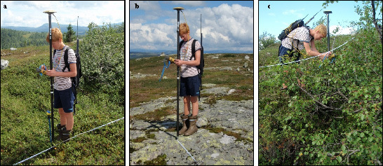
2.2. Field Measurements

2.2.1. Establishing and Recording of Ground Control Point Positions

Field work was conducted in August 2010. The coordinates of a total of 40 sample points were predetermined such that they constituted a systematic sample spaced 50 m apart within the 200 × 600 m rectangle. These 40 points were intended for subsequent sub-sampling of terrain control points and detailed terrestrial measurements. Real-time kinematic (RTK) differential Global Navigation Satellite System (GNSS) (Global Positioning System and Global Navigation Satellite System) was used to navigate to the points. A point was reached when the receiver reported a fixed solution. Two Topcon Legacy E+ 40-channel dual-frequency receivers observing both pseudo range and carrier phase were used as rover and base receivers, respectively. The base station was established at a national reference point located within the study area (Figure 1). Based on the accuracy standard for national reference points applied by the Norwegian Mapping Authority [38] and the error of the RTK routine, the accuracy (RMSE) of the location of the points in the field and the subsequent recording of terrain control points (see details below) was expected to be 1.0–1.5 cm horizontally and 1.5–2.5 cm vertically.

Figure 1. (a) Location of the study area in southern Norway (black square); (b) Design of the trial. The predefined sample points are marked as circles (n = 40) and those that were identified in field (n = 39) and terrain control points (n = 387) are shown as black dots. The green area is defined as forest according to the official N50 topographic map series. Accordingly, the light area is above the tree line. The black triangle shows the location of the national reference point of the Norwegian Mapping Authority (60°00′21.10929″N 9°01′43.97760″E, 951.904 m above sea level). Contour interval is 5 m.

Figure 1. (a) Location of the study area in southern Norway (black square); (b) Design of the trial. The predefined sample points are marked as circles (n = 40) and those that were identified in field (n = 39) and terrain control points (n = 387) are shown as black dots. The green area is defined as forest according to the official N50 topographic map series. Accordingly, the light area is above the tree line. The black triangle shows the location of the national reference point of the Norwegian Mapping Authority (60°00′21.10929″N 9°01′43.97760″E, 951.904 m above sea level). Contour interval is 5 m.

For each of the 40 sample points that were identified in the field, the intention was to establish 10 additional terrain control points. The sampling of the control points was conducted according to a strict systematic design. A measuring tape was stretched out on the ground through the initial sample point and oriented in the north-south direction by using a hand-held compass. Then a control point was established at exactly every 5 m along the measuring tape (i.e., at the 5, 10, …, 25 m mark of the tape) in the northern and southern sides of the initial sample point.

For each control point, the x, y and z coordinates were recorded with RTK GNSS measurements according to the same RTK routine as used for navigation to the sample points, see details above. Due to budget constraints, RTK GNSS was used to determine the reference coordinates for the control points as well as for the sample points mentioned above, rather than, for example, using total stations, because RTK GNSS was faster and cheaper and the errors indicated above were considered as acceptable relative to the error of the DTMs subject to analysis. Unfortunately, it was not feasible to maintain radio contact between the base station and the rover receiver for some of the control points and even one of the initial sample points. When planning the study, the aim was to collect field data from the 40 sample points and 400 control points, i.e., a total of 440 points. In practice, field data from 426 points were acquired. In this study, these 426 points were used as ground control points. The maximum distance between the base station and the ground control points was 345 m. The positional dilution of precision ranged between 1.5 and 3.2 with a mean value of 1.9. The number of satellites ranged between 6 and 13 with a mean of 11. The geographical distribution of the measured ground control points is displayed in Figure 1. For each point, three variables were recorded. They were “terrain form”, “terrain surface”, and “vegetation height”.

2.2.2. Recording of Ground Control Point Properties

Relating DTM errors to terrain form was considered important because establishment, survival, and growth of pioneer trees are hardly random processes. DTM error levels for different terrain forms may be important information when considering the likelihood of detecting occurrences of trees for certain terrain forms. Local-scale variability in a population of emerging trees in the forest-tundra ecotone is known to depend on variations in the terrain [4]. Terrain form, denoted as TFORM, was defined as a categorical variable which attained the values “flat” (TFORM_flat), “concave” (TFORM_concave), and “convex” (TFORM_convex). These classes were treated as mutually exclusive and assigned to the points by assessing the form of the terrain surface within a radius of approximately 1 m centred on the point. The spatial scale chosen for assessment of terrain form was determined to capture terrain variations that for this particular study area were anticipated to be at about the minimum scale of what the DTM would be able to capture, yet would be a meaningful scale for detection of vegetation changes in the form of small pioneer trees.

Terrain surface was intended to capture the material on the surface. The idea was that different materials would have different reflectivity because of the materials’ compactness, structure, and colour. Terrain surface, denoted as TSURF, was defined as a categorical variable with three mutually exclusive classes, namely “rock/bare” (TSURF_bare), “lichen/heather” (TSURF_heather), and “green” vegetation (TSURF_green). Heather comprised common heather (Calluna vulgaris), crowberry (Empetrum nigrum L.), cowberry (Vaccinium vitis-idaea), mountain heath (Phyllodoce caerulea), and alpine azalea (Loiseleuria procumbens), but not bilberry (Vaccinium myrtillus L.). The latter was classified as green vegetation.

Vegetation height, denoted as VEGH, was treated as a categorical variable with three classes: “<10 cm” (VEGH_<10), “10–20 cm” (VEGH_10–20), and ”>20 cm” (VEGH_>20). A summary of the field data is displayed in Table 1. Three examples of ground control points with different properties are displayed in Figure 2.

Table 1. Frequency distribution of the measured ground control points ^a on terrain form, terrain surface and vegetation height.

Terrain Form	Terrain Surface/Vegetation Height
	Rock/Bare			Lichen/Heather			Green
	<10 cm	10–20 cm	>20 cm	<10 cm	10–20 cm	>20 cm	<10 cm	10–20 cm	>20 cm
Flat	16	0	0	30	0	0	202	43	51
Concave	0	0	0	3	0	0	33	14	11
Convex	1	0	0	3	0	0	15	2	2

Note: ^a The sample points (n = 39) and terrain control points (n = 387) constitute the ground control points.

Table 1. Frequency distribution of the measured ground control points ^a on terrain form, terrain surface and vegetation height.

Terrain Form	Terrain Surface/Vegetation Height
	Rock/Bare			Lichen/Heather			Green
	<10 cm	10–20 cm	>20 cm	<10 cm	10–20 cm	>20 cm	<10 cm	10–20 cm	>20 cm
Flat	16	0	0	30	0	0	202	43	51
Concave	0	0	0	3	0	0	33	14	11
Convex	1	0	0	3	0	0	15	2	2

Note: ^a The sample points (n = 39) and terrain control points (n = 387) constitute the ground control points.

Figure 2. Examples of three ground control points with different characteristics. (a) A flat location with green vegetation surface and vegetation height 10–20 cm; (b) A flat location with rock/bare surface and vegetation height < 10 cm; (c) A concave location with green vegetation surface and vegetation height > 20 cm.

Figure 2. Examples of three ground control points with different characteristics. (a) A flat location with green vegetation surface and vegetation height 10–20 cm; (b) A flat location with rock/bare surface and vegetation height < 10 cm; (c) A concave location with green vegetation surface and vegetation height > 20 cm.

2.3. Laser Data Acquisition

Laser scanner data were acquired under leaf-on conditions on two occasions using a fixed-wing aircraft. The first acquisition took place on 24 July 2006 using an Optech ALTM 3100C laser scanner system. In the present study, this sensor was denoted as “ALTM 3100C”. Average flying altitude was 700 m above ground level and the pulse repetition frequency (PRF) was 100 kHz. For convenience, this acquisition was designated ACQ₁.

The three other ALS data acquisitions were carried out on 11 June 2007. The instrument used in 2007 was an upgraded version of the Optech ALTM 3100C used in 2006. After upgrade, the system had dual pulse capabilities, which implies that it was capable of handling two pulses in the air at a time. In this study, it was denoted as “ALTM Gemini”. It should be noticed that sensor-specific properties such as pulse width, pulse energy, and peak power were altered during upgrade (Table 2).

When planning the 2007 acquisitions, the objective was to fly the sensor in such a way that it would be possible to (1) compare acquisitions between sensors with sensor and flight properties as similar as possible (sensor comparison), (2) compare pulse repetition frequencies, and finally, (3) compare flying altitudes. All the four ALS datasets were, therefore, acquired by flying along two north-east/south-west oriented and parallel flight lines each time. The coordinates of the flight lines were as similar in the four acquisitions as practically feasible.

Table 2. Summary of laser scanner data and flight parameters of the four laser data acquisitions.

Parameter	Acquisition
	ACQ1	ACQ2	ACQ3	ACQ4
System	ALTM 3100C	ALTM Gemini	ALTM Gemini	ALTM Gemini
Pulse width	14.7 ns	>14.7 ns a	b	b
Pulse energy	69 μJ	<69 μJ a	b	b
Peak power	4.7 kW	<4.7 kW a	b	b
Wavelength	1064 nm	1064 nm	1064 nm	1064 nm
Repetition frequency	100 kHz	125 kHz	166 kHz	166 kHz
Scan frequency	70 Hz	70 Hz	70 Hz	70 Hz
Pulse mode	Single	Single	Single	Dual
Date	24 July 2006	11 June 2007	11 June 2007	11 June 2007
Mean flying altitude	700 m a.g.l.	700 m a.g.l.	700 m a.g.l.	1130 m a.g.l.
Flight speed	80 m∙s−1	75 m∙s−1	75 m∙s−1	75 m∙s−1
Max. scan angle	14°	14°	14°	10°
Max processing angle	14°	14°	14°	10°
Mean footprint diameter	18 cm	17 cm	17 cm	28 cm
Mean point density	7.7 m−2	9.1 m−2	11.0 m−2	8.4 m−2
Proportion of deleted echoes c	0%	<0.01%	0.2%	9.3%

Notes: ^a Specific values not released by Optech Inc. However, the ALTM 3100C and the ALTM Gemini are the same instruments before and after upgrade, respectively. Thus, assumptions about the pulse properties can be drawn on the basis of the change in repetition frequency. ^b Instrument specifications were not released by Optech Inc., however, pulse width will be larger than pulse width of the 125 kHz acquisition (ACQ₂), whereas pulse energy and peak power will be lower. ^c Low echoes deleted in the terrain classification, see text for explanation.

Table 2. Summary of laser scanner data and flight parameters of the four laser data acquisitions.

Parameter	Acquisition
	ACQ1	ACQ2	ACQ3	ACQ4
System	ALTM 3100C	ALTM Gemini	ALTM Gemini	ALTM Gemini
Pulse width	14.7 ns	>14.7 ns a	b	b
Pulse energy	69 μJ	<69 μJ a	b	b
Peak power	4.7 kW	<4.7 kW a	b	b
Wavelength	1064 nm	1064 nm	1064 nm	1064 nm
Repetition frequency	100 kHz	125 kHz	166 kHz	166 kHz
Scan frequency	70 Hz	70 Hz	70 Hz	70 Hz
Pulse mode	Single	Single	Single	Dual
Date	24 July 2006	11 June 2007	11 June 2007	11 June 2007
Mean flying altitude	700 m a.g.l.	700 m a.g.l.	700 m a.g.l.	1130 m a.g.l.
Flight speed	80 m∙s−1	75 m∙s−1	75 m∙s−1	75 m∙s−1
Max. scan angle	14°	14°	14°	10°
Max processing angle	14°	14°	14°	10°
Mean footprint diameter	18 cm	17 cm	17 cm	28 cm
Mean point density	7.7 m−2	9.1 m−2	11.0 m−2	8.4 m−2
Proportion of deleted echoes c	0%	<0.01%	0.2%	9.3%

Notes: ^a Specific values not released by Optech Inc. However, the ALTM 3100C and the ALTM Gemini are the same instruments before and after upgrade, respectively. Thus, assumptions about the pulse properties can be drawn on the basis of the change in repetition frequency. ^b Instrument specifications were not released by Optech Inc., however, pulse width will be larger than pulse width of the 125 kHz acquisition (ACQ₂), whereas pulse energy and peak power will be lower. ^c Low echoes deleted in the terrain classification, see text for explanation.

The major purpose of the ALS acquisitions was to study vegetation, primarily small pioneer trees. The operating parameters of the aircraft and instruments were determined for this purpose. A preliminary investigation in another study area with mature forest indicated that the best correspondence between canopy height distributions derived from the ALTM 3100C data at 100 kHz and from the ALTM Gemini could be obtained by flying the ALTM Gemini system with a 125 kHz PRF. The first of the 2007 acquisitions was, therefore, carried out with an average flying altitude of 700 m above ground level and a 125 kHz PRF. This acquisition was designated ACQ₂ and it was intended for comparisons of sensors (ALTM 3100C versus ALTM Gemini) and pulse repetition frequencies (125 versus 166 kHz).

Secondly, the ALTM Gemini sensor was flown at 700 m above ground level with a 166 kHz PRF, designated ACQ₃. This acquisition allowed comparisons of pulse repetition frequencies (125 versus 166 kHz) and flying altitudes (700 versus 1130 m above ground level). Finally, ALTM Gemini was flown at 1130 m above ground level at a PRF of 166 kHz, designated ACQ₄, and it allowed comparison of flying altitudes (700 versus 1130 m above ground level). It should be noted that dual pulse mode was required to capture data at 1130 m with 166 kHz (ACQ₄).

Seasonality will influence structure and color of the vegetation and may as a result affect the laser backscatter signal. A basic requirement for the comparison of sensors was that the trees and other ground vegetation were in a similar state on 24 July 2006 when the ALTM 3100C data were acquired and on 11 June 2007 when the ALTM Gemini data were acquired. In late July, the ground vegetation can be expected to be fully developed. In early to mid-June, the state of the ground vegetation is subject to large inter-annual variations, depending on snow conditions and temperature. It was important to have full control over the conditions when the second acquisition took place in 2007. A field visit therefore took place at 11:00 UTC on 10 June 2007—28 h before the ALTM Gemini acquisitions took place (15:20–15:55 UTC on 11 June 2007). Across the entire study area it appeared that heather and small bushes like dwarf birch (Betula nana) and willow tickets (various Salix species) were fully developed (Figure 3). So was also the grass, apart from a few wet spots where the snow had melted recently and dead grass from the previous year was still visible.

Figure 3. Photographs taken from a central part of the study area towards south (a) and north (b) showing the stage of vegetation development as observed in the field at 11:00 UTC on 10 June 2007. The ALS data were acquired at 15:20–15:55 UTC on 11 June 2007. Apart from a few wet spots with some dead grass from the previous year still visible, the ground vegetation appeared fully developed.

Figure 3. Photographs taken from a central part of the study area towards south (a) and north (b) showing the stage of vegetation development as observed in the field at 11:00 UTC on 10 June 2007. The ALS data were acquired at 15:20–15:55 UTC on 11 June 2007. Apart from a few wet spots with some dead grass from the previous year still visible, the ground vegetation appeared fully developed.

2.4. Laser Data Processing

2.4.1. Pre-Processing of Laser Data

The laser data were pre-processed by the contractor (Blom Geomatics, Norway). Planimetric coordinates (x and y) and ellipsoidic height values were computed for all laser points. Since each of the four ALS acquisitions consisted of two overlapping strips, a strip adjustment was carried out by the contractor using TerraMatch software [39]. The strip-wise elevation was corrected by a constant factor ranging from −0.130 m to +0.166 m for the individual strips [40]. The maximum correction difference between the two strips of an acquisition was 0.109 m (ACQ₄). In the strip adjustment, a constant strip-wise roll correction of 0.0023–0.0080 degrees was also applied.

The laser points used to derive the terrain models were the echoes labelled “last-of-many” and “single”. Because of the generally low vegetation in the study area most of the echoes were of the type “single”. For each of the four ALS acquisitions, TerraScan software [41] was used to classify ground points and derive terrain models. In this classification it appeared that a considerable amount of anomalous echoes (long ranges below the terrain surface) and echoes with large measurement errors were present in the data [40]. The large measurement errors were due to low energy levels at high repetition frequencies (125 and 166 kHz) and at high flying altitudes (1130 m above ground level). These echoes were identified and discarded by the contractor using standard tools in TerraScan (“low points” and “below points” algorithms). Details about the number of discarded echoes in each dataset can be found in Table 2.

2.4.2. Calculating Terrain Models

After the low echoes were discarded, triangulated irregular networks (TINs) were generated for the four ALS acquisitions using the planimetric coordinates, and corresponding height values of the last echoes classified as terrain ground points according to the progressive triangular irregular network densification algorithm [33] of TerraScan. The classification of ground points to obtain the four different TIN models was based on typical parameters used in operational projects. The “iteration distance” [41] was set to 1.0 m. The other major parameter controlling the outcome of the classification, i.e., the “iteration angle” was assigned a value of 9 degrees. The algorithm starts from below with selected seed points (lowest echoes) within grid cells of pre-defined size. These seed points are used to construct an initial TIN model. Additional echoes are then added as vertices of the TIN model in subsequent iterations in which inclusion of new vertices is controlled by the iteration angle and iteration distance. The iteration angle controls the maximum allowable angle between a potentially new vertex, its projection on a triangle plane and the closest triangle vertex. A large angle will allow greater vertical variability over short distances, with a potential risk of including, for example, above-ground vegetation echoes in the model. The iteration distance controls the maximum allowable distance between a potentially new vertex and the triangle plan and helps in avoiding big vertical jumps when the triangles are large.

In the subsequent analysis of DTM errors, the four derived TIN models were the DTMs subject to analysis.

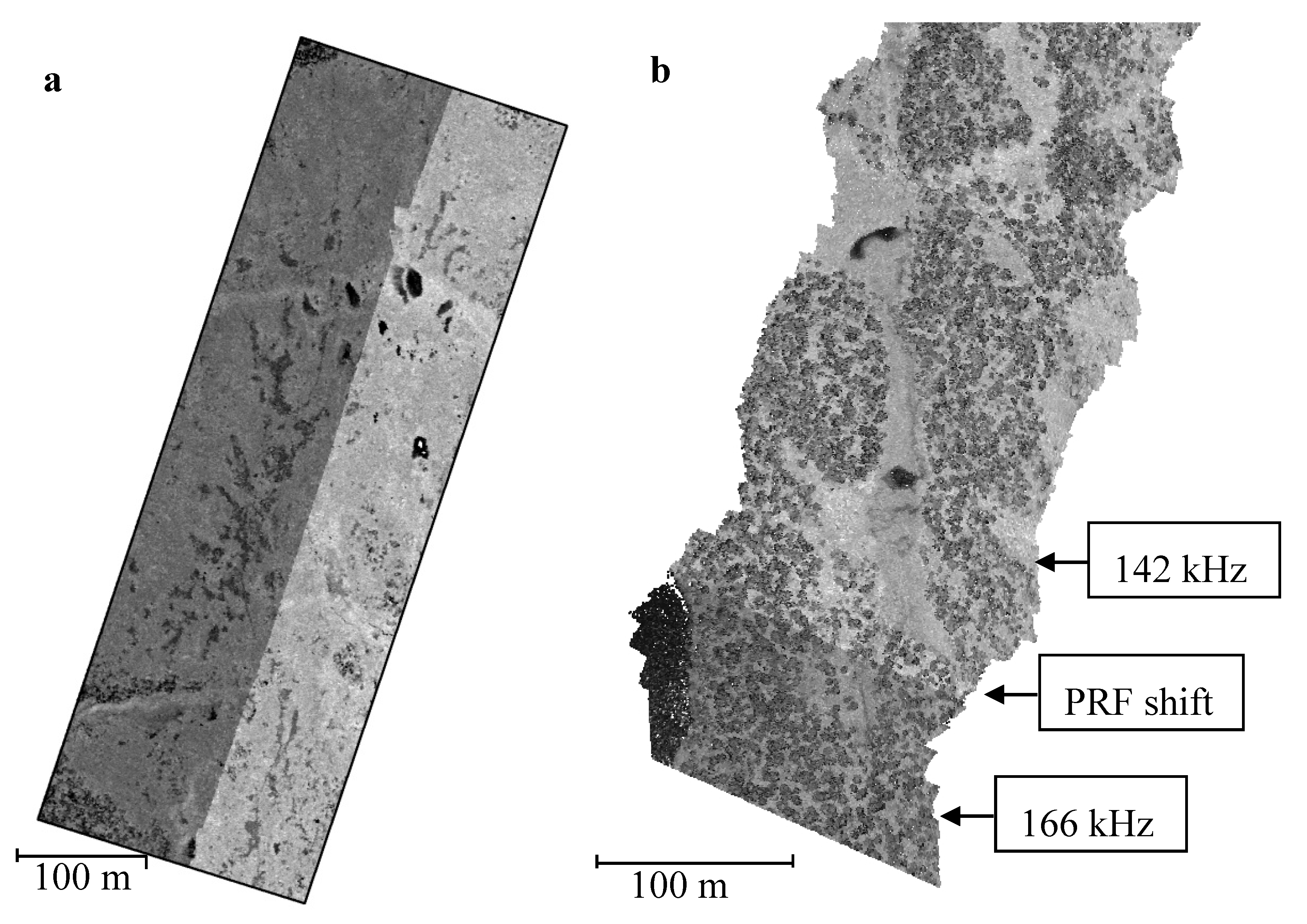
2.4.3. Identifying PRF Shifts in Dual Pulse Mode

A final manual inspection of the ALS data revealed some unexpected patterns of the backscatter intensity for ACQ₃. The entire eastern strip (Figure 4) consistently appeared to have higher intensity values than the western strip, which is important to account for in the subsequent statistical analysis. It appeared that the ALS data were acquired along the western strip at the preset PRF of 166 kHz, whereas data along the eastern strip were acquired at 142 kHz due to an automatic PRF shift activated in dual pulse mode. The automatic shift in PRF is implemented to avoid a risk of losing data when there is a rapid decrease in distance between the aircraft and the ground. This PRF was kept stable as long as the aircraft recorded data over the study area. By inspection of the data, it appeared that the PRF returned to its initial setting of 166 kHz, approximately 1.2 km south of the study area (Figure 4).

Figure 4. Illustration by backscatter intensity of the unexpected automatic shift in pulse repetition frequency (PRF) from 166 to 142 kHz for ACQ₃. (a) Backscatter intensity for the two strips of ACQ₃ over the study area. Low backscatter intensity (dark grey) is shown for the western strip flown at 166 kHz, as planned. High backscatter intensity (light grey) is seen for the eastern strip (142 kHz); (b) Illustration of where the initial PRF (166 kHz) was restored in the eastern strip, approximately 1.2 km outside the study area, by a significant drop in backscatter intensity.

Figure 4. Illustration by backscatter intensity of the unexpected automatic shift in pulse repetition frequency (PRF) from 166 to 142 kHz for ACQ₃. (a) Backscatter intensity for the two strips of ACQ₃ over the study area. Low backscatter intensity (dark grey) is shown for the western strip flown at 166 kHz, as planned. High backscatter intensity (light grey) is seen for the eastern strip (142 kHz); (b) Illustration of where the initial PRF (166 kHz) was restored in the eastern strip, approximately 1.2 km outside the study area, by a significant drop in backscatter intensity.

2.4.4. Terrain Slope Calculation

Based on each of the four processed TIN models, the slope was calculated in percent as a continuous variable at the location of the control points. However, TINs by their very nature can be spiky in terms of slope, since no smoothing is applied, especially at a sub-meter scale. Further, since the TIN models were derived from ALS data with point densities of 7.7–11.0 points∙m⁻² (Table 2), terrain slope derived from a TIN model of full density will also lead to a characterisation of the terrain at a geographical scale which may be irrelevant for the biological phenomenon motivating this study (vegetation changes represented by small pioneer trees in the boreal-alpine ecotone). Thus, the TINs were smoothed as much as possible prior to slope calculation, under the condition that the elevation at the vertices of the initial TIN models should not deviate by more than 0.2 m from the smoothed TIN models, assuming linear interpolation. This smoothing resulted in TIN models for slope calculation with 4.2%–9.7% of the initial number of vertices retained, corresponding to an average of one vertex per 4–6 m². It should be noted that a large portion of the study area was located along a fairly flat part of the mountain ridge (see Figure 1 and Figure 2b), with fewer vertices per unit area along the ridge. However, there were more vertices on the sides of the ridge where the local terrain variability was greater. Overall the study area displayed a fairly wide range of slope values (Table 3).

2.4.5. Overall Calibration of the Laser Data

Finally, a note on the calibration procedures is appropriate. The calibration affecting potential systematic shifts in terrain elevation consists of a three-stage procedure. First, the ALS instrument is typically calibrated by test flights and in the laboratory by the system producer during maintenance and upgrade (A). Secondly, a calibration is conducted in conjunction with installation in the aircraft (B). Finally, there is a daily calibration routine in which ground elevation is collected in the field in every project (C). In the current study, calibrations A-B were conducted, but not the local calibration against field control elevation, because the ALS data were mainly collected for study of vegetation (height values relative to the terrain surface). Thus, the current data may be subject to an overall shift in elevation which would not be present in a pure commercial product. However, potential systematic differences in shifts for different experimental factors (e.g., terrain form and vegetation height), which were subject to analysis in the current study, will be unaffected by overall shifts in DTM elevation.

2.5. Analysis

2.5.1. Estimation of Error Statistics

The ground control points were spatially registered to the four respective TIN models according to their coordinates. Terrain surface elevation values were computed for each control point by linear interpolation from the TINs. The relative error in elevation for each point was computed as the difference between the interpolated TIN surface elevation and the ground control elevation and denoted ε.

Several descriptive statistics were estimated for various parts of the dataset. First, the mean error between the TIN elevations and ground control points was estimated for all observations as well as for the four acquisitions and slopes. The slope was divided into six classes (Table 3). The mean error ($\overline{\epsilon }$), which quantifies the magnitude of a systematic shift in the DTM relative to the ground control points, was estimated as the mean difference between the DTM elevations and the ground control elevations according to

$$\overline{\epsilon }=\frac{1}{n}{\displaystyle \sum }_{i=1}^n{\epsilon }_i$$

(1)

where ε_i is the difference between the TIN elevation and the ground control elevation for observation i, i = 1, 2, …, n in a given subgroup of the data. Standard deviation, which quantifies the random error around the derived terrain surface, was estimated for the differences (paired observations) according to

$$s=\sqrt{\frac{{{\displaystyle \sum }}_{i=1}^n{\left({\epsilon }_i-\overline{\epsilon }\right)}^2}{n-1}}$$

(2)

Recent studies have pointed out that conventional estimators like those presented above, are not always suitable for characterising DTM errors because they assume normally distributed errors and that no outliers exist [42]. Q-Q plots of the error distributions for the four DTMs were therefore produced and inspected visually for assessment of extreme outliers and serious departure from normality. Estimates of robust error measures suited for non-normal error distributions were also provided. The applied estimators comprised the 50% sample quantile of the errors (P50_ε, i.e., the median value), which is a robust estimator for a systematic shift of the DTM [43]. Furthermore, the normalized median absolute deviation (NMAD), which can be considered an estimate for the standard deviation resilient to outliers in the error distribution [43], was estimated according to

NMAD = 1.4826 × median_i (|ε_i − P50_ε|)

(3)

Finally, the 95% quantile of the absolute value of the errors (P95_|ε|) was estimated to gauge the magnitude of the errors when excluding the 5% most extreme errors. The mentioned statistics were estimated for each acquisition for the individual terrain forms, terrain surfaces, and vegetation heights.

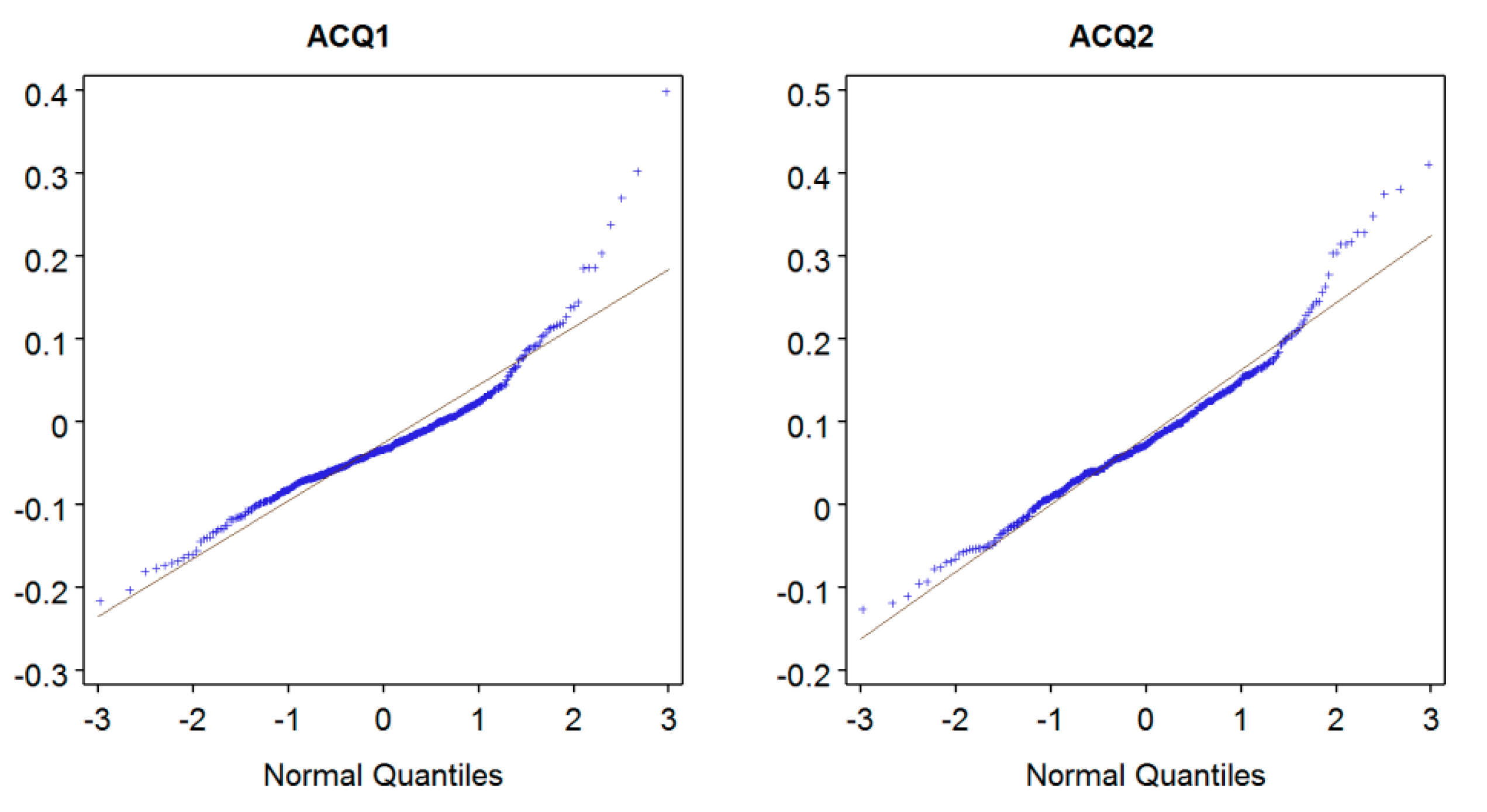
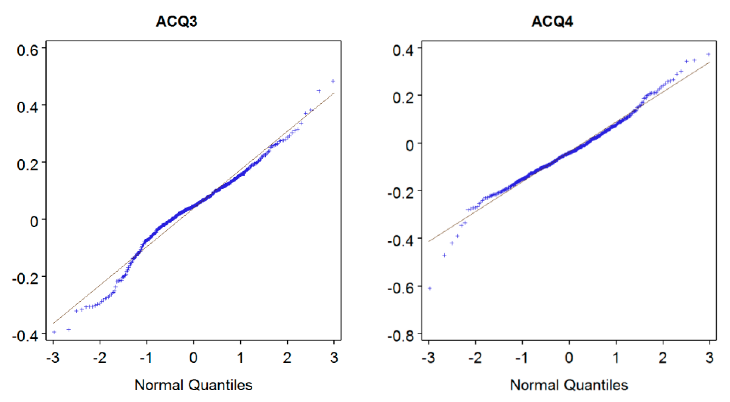
2.5.2. Regression Analysis of Errors

The contribution of the various effects (acquisition, terrain form, terrain surface, vegetation height, terrain slope) to the errors of the terrain models was assessed by regression analysis. Each of the 426 ground control points was included as four separate observations in the model, one for each DTM. These four observations for each point were likely to be intercorrelated. The model was therefore developed by means of a mixed modelling procedure to account for the hierarchical structure of the data. Further, terrain form (TFORM), terrain surface (TSURF), and vegetation height (VEGH) were included as categorical variables, while terrain slope in percent (SLOPE) was included as a continuous variable. Since it was revealed that the pulse repetition frequency for ACQ₃ had been unexpectedly and automatically shifted from 166 kHz to 142 kHz for some of the control points (see details above), the effects for this particular acquisition were allowed to be accounted for in the model. The full model can be expressed as the mean (expected value) function

$$E\left[{\epsilon }_{Qi}\right]={\beta }_0+{\alpha }_{0i}+{\beta }_{1}AC{Q_2}_{Qi}+{\beta }_{2}AC{{Q_3}_{Qi}}^{†}+{\beta }_{3}AC{{Q_3}_{Qi}}^{*}+{\beta }_{4}AC{Q_4}_{Qi}+{\beta }_{5}TFOR{M_{concave}}_{Qi}{\beta }_{6}TFOR{M_{convex}}_{Qi}+{\beta }_{7}TSUR{F_{heather}}_{Qi}+{\beta }_{8}TSUR{F_{green}}_{Qi}+{\beta }_{9}VEG{H_{10–20}}_{Qi}+{\beta }_{10}VEG{H_{>20}}_{Qi}+{\beta }_{11}SLOP{E}_{Qi}$$

(4)

where ε_Qi is the error in elevation using observations from acquisition Q, Q = {ACQ₁, ACQ₂, ACQ₃, ACQ₄} for ground control point i. The betas (β₀, β₁, …, β₁₁) are parameters for fixed effects to be estimated. Correspondingly, the alphas (α_0i) represent random effects for ground control point i. In order to account for the unexpected shift in PRF from 166 to 142 kHz for ACQ₃, ^† is used to symbolise the 142 kHz acquisition of ACQ₃ whereas ^* represents the 166 kHz acquisition of ACQ₃. The model was estimated using the MIXED procedure of the SAS statistical software package [44].

It should be noticed that the reference in the model is acquisition ACQ₁, terrain form TFORM_flat, terrain surface TSURF_bare, and vegetation height VEGH_<10. Thus, all estimated parameters for the respective variables express differences relative to this reference. The effects of, for example, the concave and convex terrain forms (TFORM_concave and TFORM_convex) relative to flat areas (TFORM_flat) will be expressed directly by the parameter estimates of the two former variables.

2.5.3. Tests of Contrast in the Regression Analysis

Contrasts were constructed in the regression analysis to test if there is a significant difference between individual acquisitions in pairs of such acquisitions (ACQ₂ versus ACQ₃; ACQ₂ versus ACQ₄; ACQ₃ versus ACQ₄). Contrasts were also constructed to test if there is a significant difference between terrain forms (TFORM_concave versus TFORM_convex), terrain surfaces (TSURF_heather versus TSURF_green), and ground vegetation heights (VEGH_10–20 versus VEGH_>20). Finally, to see if there was any effect of the unexpected change of pulse repetition frequency for ACQ₃, the difference between 142 kHz and 166 kHz was tested.

2.5.4. Goodness of Fit of the Regression Model

Because the four observations for each ground control point were likely to be intercorrelated, the conventional R² statistic does not fulfill general requirements for an R² statistic proposed by, e.g., Kvålseth [45]. Model fit was therefore assessed by the pseudo-R², which has been used for mixed models by others [46]. The pseudo-R² was computed as 1 minus the ratio between the sum of residual squares (SSR) and the corrected total sum of squares (CSST), i.e.,

$$Pseudo-R^2=1-\left(\frac{SSR}{CSST}\right)$$

(5)

3. Results

3.1. Overall Results

Visual inspection of the Q-Q plots of the error distributions (Figure 5) revealed that the departure from normality was moderate and that the extreme errors were of moderate magnitude for all the four DTMs. The extreme errors were smaller than ±0.6 m for all DTM models and even within a range of ±0.4 m for some of the models. The individual extreme errors were few in number. The error statistics assuming normally distributed errors, corresponded quite well with their robust counterparts that did not assume normally distributed errors, confirming that non-normality and extreme errors were not a serious concern in this study. Thus, the mean error ($\overline{\epsilon }$) and the 50% quantile of the errors (P50_ε) deviated by 0.04 m or less for all sub-groups of the material and in most cases with only 0.01–0.02 m (Table 3 and Table 4). Likewise, the standard deviation of the errors (s) deviated from the normalized median absolute deviation (NMAD) by a maximum of 0.11 m, while in most cases the deviation was smaller than 0.05 m (Table 3 and Table 4).

Figure 5. Normal Q-Q plot for the distribution of the individual errors (ε) between TIN surface elevation and ground control elevation for the four different TIN models.

Figure 5. Normal Q-Q plot for the distribution of the individual errors (ε) between TIN surface elevation and ground control elevation for the four different TIN models.

3.2. Detailed Results for Individual Effects

The overall mean error between the TIN elevation and the elevation of the ground control points across all ALS acquisitions was 0.01 m (Table 3), which was identical to the P50_ε value. For the four DTMs the mean error ranged between −0.04 and 0.08 m (Table 3). In the regression analysis, all the four mean errors of the individual acquisitions differed statistically from each other (p < 0.001, Table 5) significantly. The standard deviation of the errors in elevation ranged between 0.07 and 0.08 m for the 100–125 kHz acquisitions (ACQ₁–ACQ₂) and was 0.13 m for the 166 kHz acquisitions (ACQ₃–ACQ₄) (Table 3). The somewhat larger random errors for the 166 kHz acquisitions were reflected in higher values of the 95% quantile of the absolute value of the errors (P95_|ε|) (Table 3). There was no statistically significant effect of the unexpected shift in PRF from 166 to 142 kHz for ACQ₃ (p = 0.103, Table 5).

Table 3. Mean error of TIN surface elevation ($\overline{\epsilon }$), standard deviation of the errors (s), 50% quantile of the errors (P50_ε), normalized median absolute deviation (NMAD), and 95% quantile of the absolute value of the errors (P95_|ε|) for different acquisitions and terrain slopes.

Effect	n	$\overline{\epsilon }$ (m)	s (m)	P50ε (m)	NMAD (m)	P95|ε| (m)
Acquisition
700 m 100 kHz (ACQ1)	426	−0.03	0.07	−0.03	0.07	0.14
700 m 125 kHz (ACQ2)	426	0.08	0.08	0.07	0.11	0.22
700 m 166 kHz (ACQ3) a	426	0.04	0.13	0.05	0.12	0.28
1130 m 166 kHz (ACQ4)	426	−0.04	0.13	−0.04	0.12	0.25
Slope
<10%	359	0.00	0.09	0.00	0.08	0.18
10%–20%	560	0.01	0.11	0.01	0.10	0.21
20%–30%	387	0.02	0.12	0.02	0.10	0.23
30%–40%	205	0.03	0.13	0.04	0.13	0.25
40%–50%	98	0.04	0.15	0.04	0.13	0.35
>50%	95	0.05	0.16	0.04	0.16	0.32
Overall	1704	0.01	0.12	0.01	0.10	0.24

Note: ^a Comprises data acquired at 166 kHz along the western strip and data acquired at 142 kHz along the eastern strip, see Figure 4.

Table 3. Mean error of TIN surface elevation ($\overline{\epsilon }$), standard deviation of the errors (s), 50% quantile of the errors (P50_ε), normalized median absolute deviation (NMAD), and 95% quantile of the absolute value of the errors (P95_|ε|) for different acquisitions and terrain slopes.

Effect	n	$\overline{\epsilon }$ (m)	s (m)	P50ε (m)	NMAD (m)	P95|ε| (m)
Acquisition
700 m 100 kHz (ACQ1)	426	−0.03	0.07	−0.03	0.07	0.14
700 m 125 kHz (ACQ2)	426	0.08	0.08	0.07	0.11	0.22
700 m 166 kHz (ACQ3) a	426	0.04	0.13	0.05	0.12	0.28
1130 m 166 kHz (ACQ4)	426	−0.04	0.13	−0.04	0.12	0.25
Slope
<10%	359	0.00	0.09	0.00	0.08	0.18
10%–20%	560	0.01	0.11	0.01	0.10	0.21
20%–30%	387	0.02	0.12	0.02	0.10	0.23
30%–40%	205	0.03	0.13	0.04	0.13	0.25
40%–50%	98	0.04	0.15	0.04	0.13	0.35
>50%	95	0.05	0.16	0.04	0.16	0.32
Overall	1704	0.01	0.12	0.01	0.10	0.24

Note: ^a Comprises data acquired at 166 kHz along the western strip and data acquired at 142 kHz along the eastern strip, see Figure 4.

Table 4. Mean error of TIN surface elevation ($\overline{\epsilon }$), standard deviation of the errors (s), 50% quantile of the errors (P50_ε), normalized median absolute deviation (NMAD), and 95% quantile of the absolute value of the errors (P95_|ε|) for different effects (terrain form, terrain surface, vegetation height).

Acquisition	Effect	n	$\overline{\epsilon }$ (m)	s (m)	P50ε (m)	NMAD (m)	P95|ε| (m)
	Terrain form (TFORM)
700 m 100 kHz (ACQ1)	Flat	342	−0.03	0.06	−0.04	0.07	0.13
700 m 100 kHz (ACQ1)	Concave	61	0.02	0.08	0.01	0.05	0.14
700 m 100 kHz (ACQ1)	Convex	23	−0.07	0.06	−0.07	0.11	0.17
700 m 125 kHz (ACQ2)	Flat	342	0.08	0.07	0.07	0.10	0.20
700 m 125 kHz (ACQ2)	Concave	61	0.13	0.09	0.13	0.20	0.31
700 m 125 kHz (ACQ2)	Convex	23	0.01	0.10	−0.01	0.08	0.13
700 m 166 kHz (ACQ3) a	Flat	342	0.03	0.13	0.04	0.12	0.27
700 m 166 kHz (ACQ3) a	Concave	61	0.11	0.13	0.12	0.19	0.30
700 m 166 kHz (ACQ3) a	Convex	23	−0.02	0.17	−0.02	0.11	0.32
1130 m 166 kHz (ACQ4)	Flat	342	−0.04	0.12	−0.05	0.12	0.23
1130 m 166 kHz (ACQ4)	Concave	61	0.04	0.12	0.03	0.12	0.26
1130 m 166 kHz (ACQ4)	Convex	23	−0.11	0.19	−0.15	0.24	0.37
	Terrain surface (TSURF)
700 m 100 kHz (ACQ1)	Rock/bare	17	−0.09	0.04	−0.08	0.12	0.20
700 m 100 kHz (ACQ1)	Lichen/heather	36	−0.04	0.04	−0.04	0.06	0.11
700 m 100 kHz (ACQ1)	Green	373	−0.02	0.07	−0.03	0.06	0.14
700 m 125 kHz (ACQ2)	Rock/bare	17	0.01	0.06	0.00	0.08	0.12
700 m 125 kHz (ACQ2)	Lichen/heather	36	0.06	0.05	0.06	0.09	0.15
700 m 125 kHz (ACQ2)	Green	373	0.09	0.08	0.08	0.12	0.23
700 m 166 kHz (ACQ3) a	Rock/bare	17	−0.06	0.12	−0.02	0.07	0.32
700 m 166 kHz (ACQ3) a	Lichen/heather	36	−0.01	0.14	0.02	0.15	0.29
700 m 166 kHz (ACQ3) a	Green	373	0.05	0.13	0.05	0.13	0.28
1130 m 166 kHz (ACQ4)	Rock/bare	17	−0.11	0.09	−0.11	0.18	0.22
1130 m 166 kHz (ACQ4)	Lichen/heather	36	−0.06	0.08	−0.05	0.09	0.19
1130 m 166 kHz (ACQ4)	Green	373	−0.03	0.13	−0.04	0.13	0.25
	Vegetation height (VEGH)
700 m 100 kHz (ACQ1)	<10 cm	303	−0.04	0.05	−0.04	0.06	0.12
700 m 100 kHz (ACQ1)	10–20 cm	59	0.00	0.06	−0.01	0.06	0.13
700 m 100 kHz (ACQ1)	>20 cm	64	0.03	0.11	0.01	0.11	0.24
700 m 125 kHz (ACQ2)	<10 cm	303	0.07	0.07	0.07	0.10	0.17
700 m 125 kHz (ACQ2)	10–20 cm	59	0.09	0.09	0.09	0.14	0.26
700 m 125 kHz (ACQ2)	>20 cm	64	0.13	0.11	0.12	0.18	0.31
700 m 166 kHz (ACQ3) a	<10 cm	303	0.02	0.13	0.04	0.11	0.28
700 m 166 kHz (ACQ3) a	10–20 cm	59	0.07	0.12	0.06	0.14	0.26
700 m 166 kHz (ACQ3) a	>20 cm	64	0.12	0.16	0.11	0.19	0.37
1130 m 166 kHz (ACQ4)	<10 cm	303	−0.06	0.11	−0.06	0.12	0.23
1130 m 166 kHz (ACQ4)	10–20 cm	59	−0.03	0.11	−0.03	0.10	0.27
1130 m 166 kHz (ACQ4)	>20 cm	64	0.06	0.14	0.07	0.14	0.26

Note: ^a Comprises data acquired at 166 kHz along the western strip and data acquired at 142 kHz along the eastern strip, see Figure 4.

Table 4. Mean error of TIN surface elevation ($\overline{\epsilon }$), standard deviation of the errors (s), 50% quantile of the errors (P50_ε), normalized median absolute deviation (NMAD), and 95% quantile of the absolute value of the errors (P95_|ε|) for different effects (terrain form, terrain surface, vegetation height).

Acquisition	Effect	n	$\overline{\epsilon }$ (m)	s (m)	P50ε (m)	NMAD (m)	P95|ε| (m)
	Terrain form (TFORM)
700 m 100 kHz (ACQ1)	Flat	342	−0.03	0.06	−0.04	0.07	0.13
700 m 100 kHz (ACQ1)	Concave	61	0.02	0.08	0.01	0.05	0.14
700 m 100 kHz (ACQ1)	Convex	23	−0.07	0.06	−0.07	0.11	0.17
700 m 125 kHz (ACQ2)	Flat	342	0.08	0.07	0.07	0.10	0.20
700 m 125 kHz (ACQ2)	Concave	61	0.13	0.09	0.13	0.20	0.31
700 m 125 kHz (ACQ2)	Convex	23	0.01	0.10	−0.01	0.08	0.13
700 m 166 kHz (ACQ3) a	Flat	342	0.03	0.13	0.04	0.12	0.27
700 m 166 kHz (ACQ3) a	Concave	61	0.11	0.13	0.12	0.19	0.30
700 m 166 kHz (ACQ3) a	Convex	23	−0.02	0.17	−0.02	0.11	0.32
1130 m 166 kHz (ACQ4)	Flat	342	−0.04	0.12	−0.05	0.12	0.23
1130 m 166 kHz (ACQ4)	Concave	61	0.04	0.12	0.03	0.12	0.26
1130 m 166 kHz (ACQ4)	Convex	23	−0.11	0.19	−0.15	0.24	0.37
	Terrain surface (TSURF)
700 m 100 kHz (ACQ1)	Rock/bare	17	−0.09	0.04	−0.08	0.12	0.20
700 m 100 kHz (ACQ1)	Lichen/heather	36	−0.04	0.04	−0.04	0.06	0.11
700 m 100 kHz (ACQ1)	Green	373	−0.02	0.07	−0.03	0.06	0.14
700 m 125 kHz (ACQ2)	Rock/bare	17	0.01	0.06	0.00	0.08	0.12
700 m 125 kHz (ACQ2)	Lichen/heather	36	0.06	0.05	0.06	0.09	0.15
700 m 125 kHz (ACQ2)	Green	373	0.09	0.08	0.08	0.12	0.23
700 m 166 kHz (ACQ3) a	Rock/bare	17	−0.06	0.12	−0.02	0.07	0.32
700 m 166 kHz (ACQ3) a	Lichen/heather	36	−0.01	0.14	0.02	0.15	0.29
700 m 166 kHz (ACQ3) a	Green	373	0.05	0.13	0.05	0.13	0.28
1130 m 166 kHz (ACQ4)	Rock/bare	17	−0.11	0.09	−0.11	0.18	0.22
1130 m 166 kHz (ACQ4)	Lichen/heather	36	−0.06	0.08	−0.05	0.09	0.19
1130 m 166 kHz (ACQ4)	Green	373	−0.03	0.13	−0.04	0.13	0.25
	Vegetation height (VEGH)
700 m 100 kHz (ACQ1)	<10 cm	303	−0.04	0.05	−0.04	0.06	0.12
700 m 100 kHz (ACQ1)	10–20 cm	59	0.00	0.06	−0.01	0.06	0.13
700 m 100 kHz (ACQ1)	>20 cm	64	0.03	0.11	0.01	0.11	0.24
700 m 125 kHz (ACQ2)	<10 cm	303	0.07	0.07	0.07	0.10	0.17
700 m 125 kHz (ACQ2)	10–20 cm	59	0.09	0.09	0.09	0.14	0.26
700 m 125 kHz (ACQ2)	>20 cm	64	0.13	0.11	0.12	0.18	0.31
700 m 166 kHz (ACQ3) a	<10 cm	303	0.02	0.13	0.04	0.11	0.28
700 m 166 kHz (ACQ3) a	10–20 cm	59	0.07	0.12	0.06	0.14	0.26
700 m 166 kHz (ACQ3) a	>20 cm	64	0.12	0.16	0.11	0.19	0.37
1130 m 166 kHz (ACQ4)	<10 cm	303	−0.06	0.11	−0.06	0.12	0.23
1130 m 166 kHz (ACQ4)	10–20 cm	59	−0.03	0.11	−0.03	0.10	0.27
1130 m 166 kHz (ACQ4)	>20 cm	64	0.06	0.14	0.07	0.14	0.26

Note: ^a Comprises data acquired at 166 kHz along the western strip and data acquired at 142 kHz along the eastern strip, see Figure 4.

Table 5. Fixed effects and tests of contrasts in the regression analysis of the error in TIN surface elevation (ε) estimated according to Equation (4).

Coefficient	Estimate	p-Value
Intercept (β0)	−0.098	<0.001
ACQ2	0.107	<0.001
ACQ3, 142 kHz a	0.049	<0.001
ACQ3, 166 kHz a	0.068	<0.001
ACQ4	−0.010	0.066
TFORMconcave	0.058	0.009
TFORMconvex	−0.050	0.014
TSURFheather	0.045	0.020
TSURFgreen	0.055	0.017
VEGH10–20	0.024	0.014
VEGH>20	0.081	<0.001
SLOPE	0.003E-3	0.981
Tests of contrasts:
ACQ2 versus ACQ3		<0.001
ACQ2 versus ACQ4		<0.001
ACQ3 versus ACQ4		<0.001
ACQ3: 142 kHz versus 166 kHz		0.103
TFORMconcave versus TFORMconvex		<0.001
TSURFheather versus TSURFgreen		0.400
VEGH10–20 versus VEGH>20		<0.001
Pseudo-R2	0.30

Note: ^a Comprises data acquired at 166 kHz along the western strip and data acquired at 142 kHz along the eastern strip, see Figure 4.

Table 5. Fixed effects and tests of contrasts in the regression analysis of the error in TIN surface elevation (ε) estimated according to Equation (4).

Coefficient	Estimate	p-Value
Intercept (β0)	−0.098	<0.001
ACQ2	0.107	<0.001
ACQ3, 142 kHz a	0.049	<0.001
ACQ3, 166 kHz a	0.068	<0.001
ACQ4	−0.010	0.066
TFORMconcave	0.058	0.009
TFORMconvex	−0.050	0.014
TSURFheather	0.045	0.020
TSURFgreen	0.055	0.017
VEGH10–20	0.024	0.014
VEGH>20	0.081	<0.001
SLOPE	0.003E-3	0.981
Tests of contrasts:
ACQ2 versus ACQ3		<0.001
ACQ2 versus ACQ4		<0.001
ACQ3 versus ACQ4		<0.001
ACQ3: 142 kHz versus 166 kHz		0.103
TFORMconcave versus TFORMconvex		<0.001
TSURFheather versus TSURFgreen		0.400
VEGH10–20 versus VEGH>20		<0.001
Pseudo-R2	0.30

Note: ^a Comprises data acquired at 166 kHz along the western strip and data acquired at 142 kHz along the eastern strip, see Figure 4.

According to the regression analysis, the mean error differed significantly between the three terrain forms: flat, concave, and convex (Table 5). The TIN elevations were 0.058 m (p = 0.009) higher above the control heights for concave surfaces as compared to flat surfaces. Similarly, the TIN elevations for flat surfaces were 0.050 m (p = 0.014) higher above the control heights compared to convex surfaces Consequently, the difference between the concave and convex surfaces was on average 0.108 m (p < 0.001) since the effects are additive. This finding indicates that the TIN models were not fully capable of following the terrain variation at the fine geographical scale deemed relevant for detecting vegetation changes in the form of small pioneer trees. Potential causes for these patterns of mean errors for different terrain forms are: (1) the limited probability of hitting the absolute bottom of a terrain depression and the absolute peak of a convex surface, even when the point density is high; further, (2) for the geographical scale considered in the current study (~1 m, see details in Section 2.2.2), the spatial extent of an individual laser footprint (0.17–0.28 m, Table 2) represents an inherent averaging of the elevation within a footprint, although the central part of a footprint will dominate the footprint’s elevation due to the uneven (Gaussian) distribution of energy across a footprint; and lastly, (3) there is an algorithm-specific effect that should be kept in mind. For the TIN-based algorithm applied in the current study, linear interpolation was used to compute elevation in-between vertices of a triangle. If there is a non-linear curvature of the terrain, linear interpolation may lead to those error patterns reported above. Other algorithms, like, for example, those based on certain forms of splines may therefore give slightly different results at very fine geographical scales. Non-linear interpolation could even have been used with the current TIN models.

The regression analysis revealed that the mean errors were less related to terrain surface characteristics than to terrain form. The difference between TIN elevations and ground control did not differ significantly between vegetated surfaces, i.e., surfaces with heather and green vegetation, respectively (p = 0.400, Table 5). However, there was a statistically significant effect of bare rock relative to the vegetated surfaces of 0.045–0.055 m (p = 0.017–0.020), with the TIN surfaces for vegetated areas located relatively higher than for bare rock.

The effect of vegetation height on TIN elevation was very pronounced. The TIN elevations relative to the ground control elevation for the tallest vegetation (>20 cm) was 0.057 m (p < 0.001) higher than for the intermediate vegetation height class (10–20 cm) and 0.081 m (p < 0.001) higher than for the lowest vegetation (<10 cm), which are reasonable and logical findings.

Detailed studies of the errors for different terrain forms, terrain surfaces, and vegetation heights for each individual acquisition (Table 4) revealed that random errors (standard deviation) tended to be larger for concave and convex terrain forms than for flat surfaces, regardless of acquisition. For flat surfaces the standard deviation ranged from 0.06 to 0.13 m, whereas for concave and convex surfaces corresponding standard errors were 0.06–0.19 m. Likewise, the standard deviations across all acquisitions tended to be higher for green vegetation than for the other vegetation types, presumably because green vegetation had a higher proportion of tall ground vegetation than the other surface types (Table 1). The tallest ground vegetation (>20 cm) showed, indeed, the highest standard deviations among all the sub-groups of the three experimental factors, with a standard deviation ranging between 0.11 and 0.16 m.

The analysis showed that the effect of slope on the difference between TIN elevation and ground control elevation was not statistically significant (p = 0.981, Table 5). The standard deviation seemed to be relatively stable across the entire range of slope angles (Table 3).

4. Discussion

4.1. General Considerations

The analysis showed that there was a mean error of −0.04 to 0.08 m (Table 3) for the various ALS-derived DTMs. As noted above, the so-called daily calibration routine, by which ground elevation is collected in the field in the survey area, was ignored in the current study. Such global calibrations aim at eliminating the overall shift in the modelled terrain surface, but local effects may remain even when a global calibration is undertaken. The main merit of the current study is (1) the quantification of the relative effects of the various factors affecting the surface elevation and (2) the reported random errors, since these quantities are unaffected by the overall calibration. Thus, some caution should be exercised when assessing the mean errors for the entire material and for individual classes, since these quantities most likely have been affected by systematic shifts that are expected to be reduced in operational projects by daily calibration.

Further, the error of the ground control itself deserves some attention. As noted above, the accuracy of the ground control was expected to be 1.0–1.5 cm horizontally and 1.5–2.5 cm vertically. The vertical accuracy (RMSE) is around 10%–35% of, for example, the reported standard deviation of the four DTMs (0.07–0.13 m, Table 3) and obviously less than 10%–35% of the accuracy (RMSE) of the DTMs. The magnitude of the reported standard deviation of the modelled terrain surfaces is therefore only marginally affected by the uncertainty of the ground control, and seems to satisfy generally recommended standards of at least three times more accurate positions of the control points than the DTMs being evaluated [43].

The noticeable increase in random errors with increasing PRFs was as expected. It is worth noting though, that while the standard deviation was fairly stable for 100 and 125 kHz (0.07–0.08 m), it increased substantially for the 166 kHz acquisitions (0.13 m). The terrain models derived from the 166 kHz acquisition at 1130 m flying altitude (ACQ₄) in particular would most likely have suffered from much more serious errors had not 9.3% (Table 2) of all echoes been deleted from the dataset. The standard deviation of the terrain models of the dual pulse mode data is therefore overly optimistic compared to an operational survey with less intensive and time-consuming manual inspection of the data. There was only a marginal or negligible effect of varying flying altitude on the standard deviation, but it should be noted that all acquisitions were carried out at relatively low flying altitudes.

4.2. Consequences for Vegetation Monitoring

This study has contributed to a quantification of the uncertainty of the terrain surface. An overall standard deviation of around 0.07–0.15 m seems to be achievable in an operational context under robust sensor and flying configurations (Table 3). For certain surfaces, such as flat and non-vegetated (rock/bare), or low vegetation areas (lichen/heather; <20 cm tall) (Table 5), the random errors may be reduced even more—to a standard deviation of, say, 0.05–0.10 m. This represents a similar or slightly smaller random error than previously reported for vegetated but tree-less surfaces (0.16 m [27]; 0.10–0.12 m [28]) and under forest canopies (0.20 m [7]). Taller ground vegetation will tend to reduce this precision, which is also consistent with previous findings [26]. These numbers exemplify the lower limits of what possibly can be expected to be detected in terms of changes in low vegetation over time.

Nevertheless, there are two particular factors in the current experiment that may merit some attention. First, the study was restricted to a rather small area of 0.12 km². Under operational conditions, literally thousands of square kilometres may be mapped during several acquisitions, resulting in greater variability in land forms and terrain morphology influencing the overall quality of the DTM. Second, the scanning angle was restricted to 14° in three of the ALS acquisitions and 10° in the fourth acquisition (Table 2). In operational projects, at least for terrain mapping, the scanning angle is often larger than the ones used in the current study. It is well known that laser shots closer to nadir will have a higher accuracy due to the smaller incidence angle with the terrain, and a reduction in the propagation of orientation (roll, pitch, and yaw) and scan angle errors into the coordinates. Thus, the errors reported in this study are likely to be in the lower range of what can be expected in surveys on larger scales.

The main focus of this study was to quantify DTM errors that may influence the success of detection of changes in low vegetation, in particular pioneer trees in the boreal-alpine ecotone. It was emphasised that the context was operational monitoring, which often will involve data from different sensors and acquisitions and use of commercially available algorithms to derive the DTMs as they are applied by commercial data vendors. Therefore, the algorithm by Axelsson [33] was the only one considered in this study. As shown by, e.g., Meng et al. [32], other algorithms may produce different results and the differences between algorithms may even vary with some of the factors examined in the current study, like, for example, terrain form. Nevertheless, for a given ALS acquisition, systematic shifts in the DTM in particular—caused by any of the factors under study in the current analysis or by differences between terrain classification algorithms—may not necessarily be a serious concern because the relative height above the terrain surface of vegetation echoes indicating a tree may still be unaffected by systematic errors. However, for monitoring (estimation of change over time) it has been advocated that a common DTM should be applied over time to reduce the influence of random differences in the DTMs on the estimated vegetation response [47]. In a sub-alpine environment in which the trees exist close to their tolerance limits, the annual height growth may be rather small, say, 0–5 cm per year [14]. Significant systematic shifts in the DTMs in the ranges found in this study may therefore become important because they may be of the same magnitude as the annual change in tree height which one would want to quantify. It therefore remains an open question if change estimation for slow-growing and low vegetation in environments like the boreal-alpine ecotone and the arctic forest-tundra interface, should be based on a common DTM over time to reduce the influence of random DTM errors, or, as an alternative, separate DTMs for each point in time should be used to reduce the influence of systematic errors in the DTMs.

The random errors associated with the DTM surface define a lower limit of the potential for detection of small trees according to ALS-derived height values. Based on the current findings, a 95% confidence bound around the modelled terrain surface would be approximately 0.15–0.30 m. For the smallest trees (<1 m in height) that were analyzed in the tree study conducted in the current study area, [16] it was reported that 35%–59% of the trees were hit by at least one laser pulse resulting in a positive height value, i.e., indicating an object located above the modelled terrain surface. Presumably, most of these trees were in the upper end of the 0–1 m range, because for those trees in the 0–1 m height range that were hit by at least one pulse the maximum recorded echo height underestimated the tree height measured in the field by approximately 0.5 m. For the smallest trees, say, <0.3 m in height, terrain model uncertainty, pulse density and pulse travel distance from the apex of a tree to an echo is triggered (with discrete return systems) are critical factors limiting the ability to measure tree height by ALS. Higher pulse densities than those used in the current studies can mitigate the sampling density problem. Full waveform systems may help improve the sensitivity of the height recording. Thus, 0.15–0.30 m in height seems to remain a lower bound of tree sizes that one potentially can expect to detect under ideal conditions. For certain terrain forms, like terrain depressions with tall ground vegetation, even these numbers may be overly optimistic. For monitoring of tree migration it must be assumed that positive detection may lag a few years behind the real migration, say, at least 5–15 years depending on the annual tree growth.

4.3. A Comment on Slope Effects

Different terrain characteristics, as represented by aspect and slope, have an influence on the potential presence and height growth of small pioneer trees [4,48,49]. It is therefore important that trees can be identified equally well on slopes as in more flat terrain in order to avoid bias in estimates of tree recruitment in the boreal-alpine ecotone. The current analysis showed that the effect of slope was not significant in the statistical sense—at least not for the moderate range in slope values that is present in the current study area. Clearly, common causes of elevation errors in steep terrain, like offset in the x, y plane, were not very pronounced due to the gentle terrain.

Further, the relatively stable DTM standard deviation across slope angles suggests that success in vegetation change detection for moderate slopes is hardly influenced by the slope. It should be noted though, that a previous study indicated a somewhat faster deterioration of the random errors with increasing slopes [35]. Surfaces with rough terrain and discontinuous slopes are also still identified as being problematic to model with most ground filtering algorithms [25]. This should be kept in mind for vegetation studies under more challenging topographic conditions than those experienced in the current study.

5. Conclusions

This study has demonstrated that a terrain model standard deviation of 0.15 m or better can be achieved from ALS data with densities of ~8–10 pulses∙m⁻² in fairly tree-less areas in the boreal-alpine ecotone with gentle terrain, provided that the laser is operated at a robust pulse repetition frequency (low noise level) and moderate flying altitudes. Increasing pulse repetition frequency will tend to increase the random errors. Systematic shifts in a terrain model will be impacted by terrain form, the type of ground vegetation, and its height. Statistically significant effects of these factors in the range of up to −0.11 to 0.13 m were found in this study. Terrain models will tend to be positively biased for concave surfaces and negatively biased for convex surfaces. The mean difference between these two extreme terrain forms relative to the ground control was 0.108 m. Tall ground vegetation will tend to elevate the modelled terrain surface. It was found that the terrain models relative to the ground control elevation were systematically shifted 0.081 m upwards for tall vegetation (>20 cm) compared to low vegetation (<10 cm). However, the random errors of a terrain model are only to a limited extent influenced by these factors, except for taller ground vegetation, for which one must expect a higher uncertainty of the modelled terrain surface.

References

1. Zheng, D.; Freeman, M.; Bergh, J.; Røsberg, I.; Nilsen, P. Production of Picea abies in South-East Norway in response to climate change: A case study using process-based model simulation with field validation. Scand. J. For. Res. 2002, 17, 35–46. [Google Scholar]
2. Kullman, L. Late Holeocene reproductional patterns of Pinus sylvestris and Picea abies at the forest limit in central Sweden. Can. J. Bot. 1986, 64, 1682–1690. [Google Scholar]
3. Kullman, L. Tree line population monitoring of Pinus sylvestris in the Swedish Scandes, 1973–2005: Implications for tree line theory and climate change ecology. J. Ecol. 2007, 95, 41–52. [Google Scholar]
4. Danby, R.K.; Hik, D.S. Variability, contigency and rapid change in recent subarctic alpine tree line dynamics. J. Ecol. 2007, 95, 352–363. [Google Scholar]
5. Soja, A.J.; Tchebakova, N.M.; French, N.N.F.; Flannigan, M.D.; Shugart, H.H.; Stocks, B.J.; Sukhinin, A.I.; Parfenova, E.I.; Chapin, F.S., III; Stackhouse, P.W., Jr. Climate-induced boreal forest change: Predictions versus current observations. Glob. Planet. Chang. 2007, 56, 274–296. [Google Scholar]
6. Callaghan, T.V.; Werkman, B.R.; Crawford, R.M.M. The tundra-taiga interface and its dynamics: Concepts and applications. Ambio 2002, 12, 6–14. [Google Scholar]
7. Hyyppä, J.; Hyyppä, H.; Leckie, D.; Gougeon, F.; Yu, X.; Maltamo, M. Review of methods of small-footprint airborne laser scanning for extracting forest inventory data in boreal forests. Int. J. Remote Sens. 2008, 29, 1339–1366. [Google Scholar]
8. McRoberts, R.E.; Andersen, H.-E.; Næsset, E. Using airborne laser scanning data to support forest sample surveys. In Forestry Applications of Airborne Laser Scanning; Maltamo, M., Næsset, E., Vauhkonen, J., Eds.; Springer: Dordrecht, The Netherlands, 2014; pp. 269–292. [Google Scholar]
9. Maltamo, M.; Packalen, P. Species-specific management inventory in Finland. In Forestry Applications of Airborne Laser Scanning; Maltamo, M., Næsset, E., Vauhkonen, J., Eds.; Springer: Dordrecht, The Netherlands, 2014; pp. 241–252. [Google Scholar]
10. Næsset, E. Area-based inventory in Norway—From innovation to an operational reality. In Forestry Applications of Airborne Laser Scanning; Maltamo, M., Næsset, E., Vauhkonen, J., Eds.; Springer: Dordrecht, The Netherlands, 2014; pp. 215–240. [Google Scholar]
11. Vauhkonen, J.; Rombouts, J.; Maltamo, M. Inventory of forest plantations. In Forestry Applications of Airborne Laser Scanning; Maltamo, M., Næsset, E., Vauhkonen, J., Eds.; Springer: Dordrecht, The Netherlands, 2014; pp. 253–268. [Google Scholar]
12. Hill, R.A.; Hinsley, S.A.; Broughton, R.K. Assessing habitats and organism-habitat relationships by airborne laser scanning. In Forestry Applications of Airborne Laser Scanning; Maltamo, M., Næsset, E., Vauhkonen, J., Eds.; Springer: Dordrecht, The Netherlands, 2014; pp. 335–356. [Google Scholar]
13. Müller, J.; Vierling, K. Assessing biodiversity by airborne laser scanning. In Forestry Applications of Airborne Laser Scanning; Maltamo, M., Næsset, E., Vauhkonen, J., Eds.; Springer: Dordrecht, The Netherlands, 2014; pp. 357–374. [Google Scholar]
14. Næsset, E.; Nelson, R. Using airborne laser scanning to monitor tree migration in the boreal-alpine transition zone. Remote Sens. Environ. 2007, 110, 357–369. [Google Scholar]
15. Nyström, M.; Holmgren, J.; Olsson, H. Prediction of tree biomass in the forest-tundra ecotone using airborne laser scanning. Remote Sens. Environ. 2012, 123, 271–279. [Google Scholar]
16. Næsset, E. Influence of terrain model smoothing and flight and sensor configurations on detection of small pioneer trees in the boreal–alpine transition zone utilizing height metrics derived from airborne scanning lasers. Remote Sens. Environ. 2009, 113, 2210–2223. [Google Scholar]
17. Thieme, N.; Bollandsås, O.M.; Gobakken, T.; Næsset, E. Detection of small single trees in the forest-tundra ecotone using height values from airborne laser scanning. Can. J. Remote Sens. 2011, 37, 264–274. [Google Scholar]
18. Stumberg, N.; Ørka, H.O.; Bollandsås, O.M.; Gobakken, T.; Næsset, E. Classifying tree and nontree echoes from airborne laser scanning in the forest-tundra ecotone. Can. J. Remote Sens. 2012, 38, 655–666. [Google Scholar]
19. Stumberg, N.; Hauglin, M.; Bollandsås, O.M.; Gobakken, T.; Næsset, E. Improving classification of airborne laser scanning echoes in the forest-tundra ecotone using geostatistical and statistical measures. Remote Sens. 2014, 6, 4582–4599. [Google Scholar]
20. Stumberg, N.; Bollandsås, O.M.; Gobakken, T.; Næsset, E. Automatic detection of small single trees in the forest-tundra ecotone using airborne laser scanning. Remote Sens. 2014, 6, 10152–10170. [Google Scholar]
21. Rees, W.G. Characterisation of arctic treelines by lidar and multispectral imagery. Polar Rec. 2007, 43, 345–352. [Google Scholar]
22. Kraus, K.; Pfeifer, N. Determination of terrain models in wooded areas with airborne laser scanner data. ISPRS J. Photogramm. Remote Sens. 1998, 53, 193–203. [Google Scholar]
23. Hodgson, M.E.; Jensen, J.; Raber, G.; Tullis, J.; Davis, B.A.; Thompson, G.; Schuckman, K. An evaluation of Lidar-derived elevation and terrain slope in leaf-off conditions. Photogramm. Eng. Remote Sens. 2005, 71, 817–823. [Google Scholar]
24. Raber, G.T.; Jensen, J.R.; Hodgson, M.E.; Tullis, J.A.; Davis, B.A.; Berglund, J. Impact of Lidar nominal post-spacing on DEM accuracy and flood zone delineation. Photogramm. Eng. Remote Sens. 2007, 73, 793–804. [Google Scholar]
25. Meng, X.; Currit, N.; Zhao, K. Ground filtering algorithms for airborne LiDAR data: A review of critical issues. Remote Sens. 2010, 2, 833–860. [Google Scholar]
26. Pfeifer, N.; Gorte, B.; Elberink, S.O. Influences of vegetation on laser altimetry—Analysis and correction approaches. Int. Arch. Photogramm. Remote Sens. Spat. Inf. Sci. 2004, 36, 283–287. [Google Scholar]
27. Reutebuch, S.E.; McGaughey, R.J.; Andersen, H.E.; Carson, W.W. Accuracy of a high-resolution lidar terrain model under a conifer forest canopy. Can. J. Remote Sens. 2003, 29, 527–535. [Google Scholar]
28. Hopkinson, C.; Chasmer, L.E.; Sass, G.; Creed, I.F.; Sitar, M.; Kalbfleisch, W.; Treitz, P. Vegetation class dependent errors in lidar ground elevation and canopy height estimates in a boreal wetland environment. Can. J. Remote Sens. 2005, 31, 191–206. [Google Scholar]
29. Mongus, D.; Žalik, B. Parameter-free ground filtering of LiDAR data for automatic DTM generation. ISPRS J. Photogramm. Remote Sens. 2012, 67, 1–12. [Google Scholar]
30. Susaki, J. Adaptive slope filtering of airborne LiDAR data in urban areas for digital terrain model (DTM) generation. Remote Sens. 2012, 4, 1804–819. [Google Scholar]
31. Tinkham, W.T.; Huang, H.; Smith, A.M.S.; Shrestha, R.; Falkowski, M.J.; Hudak, A.T.; Link, T.E.; Glenn, N.F.; Marks, D.G. A comparison of two open source LiDAR surface classification algorithms. Remote Sens. 2011, 3, 638–649. [Google Scholar]
32. Meng, X.; Currit, N.; Zhao, K. Ground filtering algorithms for airborne LiDAR data: A review of critical issues. Remote Sens. 2010, 2, 833–860. [Google Scholar]
33. Axelsson, P. Dem generation from laser scanner data using adaptive tin models. Int. Arch. Photogramm. Remote Sens. Spat. Inf. Sci. 2000, 33(B4), 111–118. [Google Scholar]
34. Hodgson, M.E.; Bresnahan, P. Accuracy of airborne lidar-derived elevation: Empirical assessment and error budget. Photogramm. Eng. Remote Sens. 2004, 70, 331–339. [Google Scholar]
35. Hyyppä, H.; Yu, X.; Hyyppä, J.; Kaartinen, H.; Honkavaara, E.; Rönnholm, P. Factors affecting the quality of DTM generation in forested areas. In Proceedings of ISPRS Workshop on Laser Scanning 2005, Enschede, The Netherlands, 12–14 September 2005; Volume XXXVI, pp. 85–90.
36. Bollandsås, O.M.; Risbøl, O.; Ene, L.T.; Nesbakken, A.; Gobakken, T.; Næsset, E. Using airborne small-footprint laser scanner data for detection of cultural remains in forests: An experimental study of the effects of pulse density and DTM smoothing. J. Archaeol. Sci. 2012, 39, 2733–2743. [Google Scholar]
37. Sithole, G.; Vosselmann, G. Experimental comparison of filter algorithms for bare-earth extraction from airborne laser scanning point clouds. ISPRS J. Photogramm. Remote Sens. 2004, 59, 85–101. [Google Scholar]
38. Kartverket. Grunnlagsnett. Versjon 1.1, Desember 2009. Norwegian Mapping Authority, 2009; p. 29. Available online: http://www.kartverket.no/Documents/Standard/Bransjestandarder%20utover%20SOSI/grunnlag.pdf (accessed on 3 March 2014).
39. Terrasolid. TerraMatch User’s Guide; Terrasolid Ltd.: Jyvaskyla, Finland, 2014; p. 89. Available online: http://www.terrasolid.com/download/tmatch.pdf (accessed on 5 March 2015).
40. Blom. Rapport BNO07757, Veggli; Project Report to Client; Blom Geomatics As: Oslo, Norway, 2007; Unpublished; p. 10. [Google Scholar]
41. Terrasolid. TerraScan User’s Guide. Terrasolid Ltd.: Jyvaskyla, Finland, 2014; p. 485. Available online: https://www.terrasolid.com/download/tscan.pdf (accessed on 5 March 2014).
42. Zandbergen, P.A. Positional accuracy of spatial data: Non-normal distributions and a critique of the national standard for spatial data accuracy. Trans. GIS 2008, 12, 103–130. [Google Scholar]
43. Höhle, J.; Höhle, M. Accuracy assessment of digital elevation models by means of robust statistical methods. ISPRS J. Photogramm. Remote Sens. 2009, 64, 398–406. [Google Scholar]
44. SAS. SAS OnlineDoc®, Version 9.2; SAS Institute Inc.: Cary, NC, USA, 2007.
45. Kvålseth, T.O. Cautionary note about R2. Am. Stat. 1985, 39, 279–285. [Google Scholar]
46. Bollandsås, O.M.; Næsset, E. Weibull models for single tree increment of Norway spruce, Scots pine, birch, and other broadleaves in Norway. Scand. J. For. Res. 2009, 24, 55–67. [Google Scholar]
47. St-Onge, B.; Vepakomma, U. Assessing forest gap dynamics and growth using multi-temporal laser-scanner data. Int. Arch. Photogramm. Remote Sens. Spat. Inf. Sci. 2004, 36(Part 8), 173–178. [Google Scholar]
48. Boisvenue, C.; Temesgen, H.; Marshall, P. Selecting a small tree height growth model for mixed-species stands in the southern interior of British Columbia, Canada. For. Ecol. Manag. 2004, 202, 301–312. [Google Scholar]
49. Mast, J.N.; Veblen, T.T.; Hodgson, M.E. Tree invasion within a pine/grassland ecotone: An approach with historic aerial photography and GIS modeling. For. Ecol. Manag. 1997, 93, 181–194. [Google Scholar]