
Topo-Bathymetric LiDAR for Monitoring River Morphodynamics and Instream Habitats—A Case Study at the Pielach River


Abstract
:
1. Introduction
Related Work
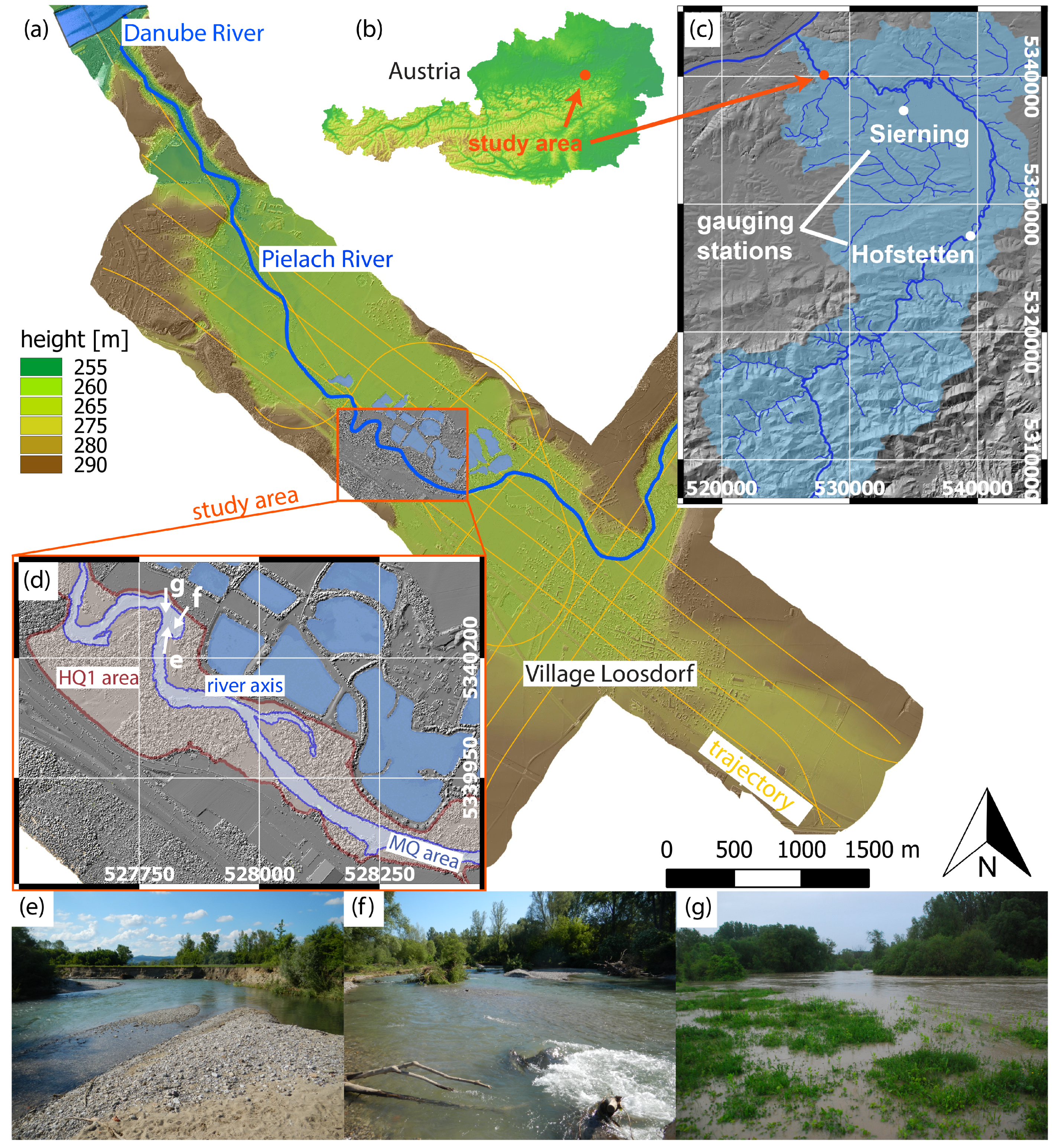
2. Study Area and Data Sets


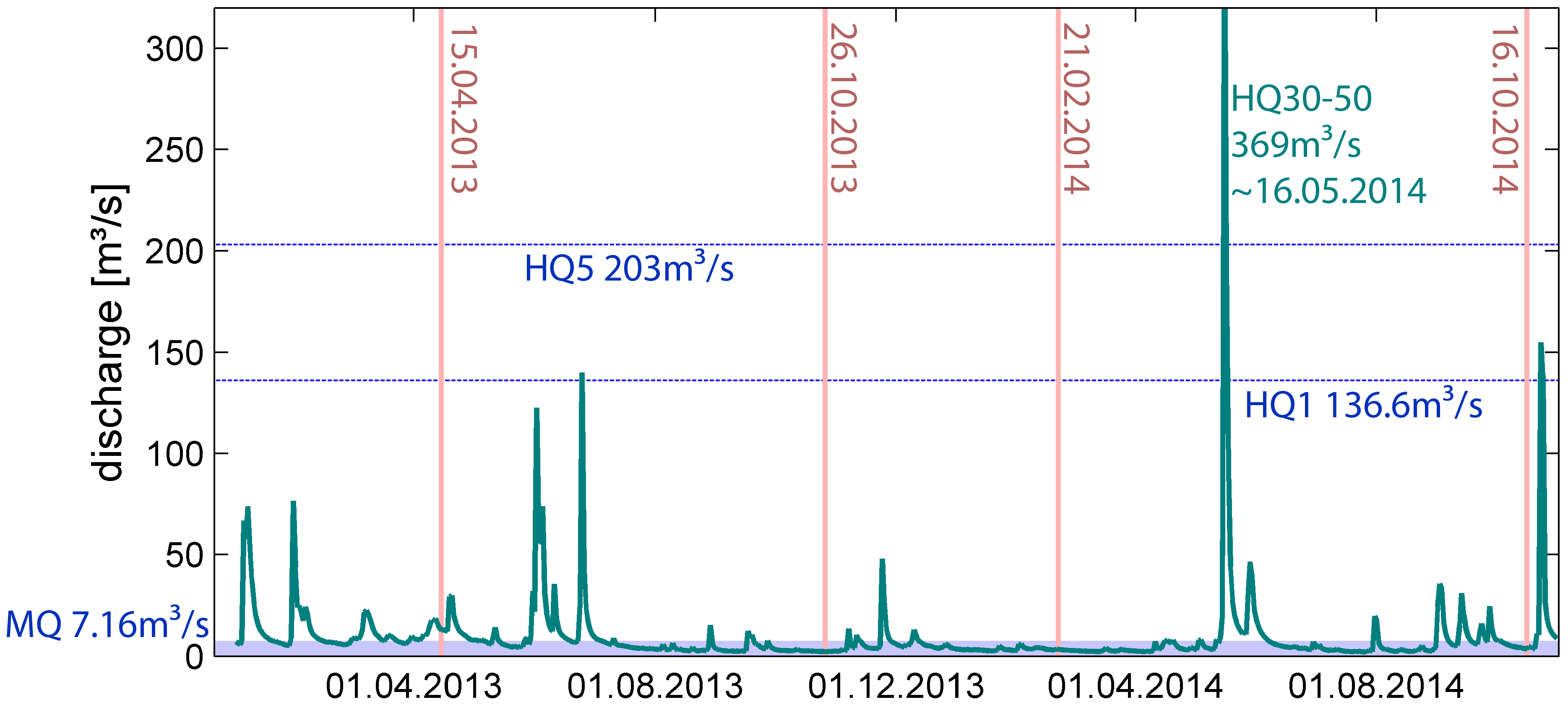
| Annuality | MQ | HQ1 | HQ5 | HQ10 | HQ30 | HQ100 |
|---|---|---|---|---|---|---|
| Discharge [m3 ·s−1] | 7.16 | 136.6 | 203 | 261 | 347 | 440 |

| Flight Date | Sensor | Q [m3 ·s−1] | Point Density [points/m2] | Precision [m] | Accuracy [m] | Foliage |
|---|---|---|---|---|---|---|
| 15 April 2013 | VQ-820-G | 12.2 | 12 | 0.016 | 0.000 | leaf-off |
| 26 October 2014 | VQ-820-G | 2.2 | 18 | 0.019 | 0.015 | leaf-on |
| 21 February 2014 | VQ-820-G | 3.4 | 25 | 0.018 | 0.017 | leaf-off |
| 16 October 2014 | VQ-880-G | 3.7 | 22 | 0.019 | 0.019 | leaf-on |
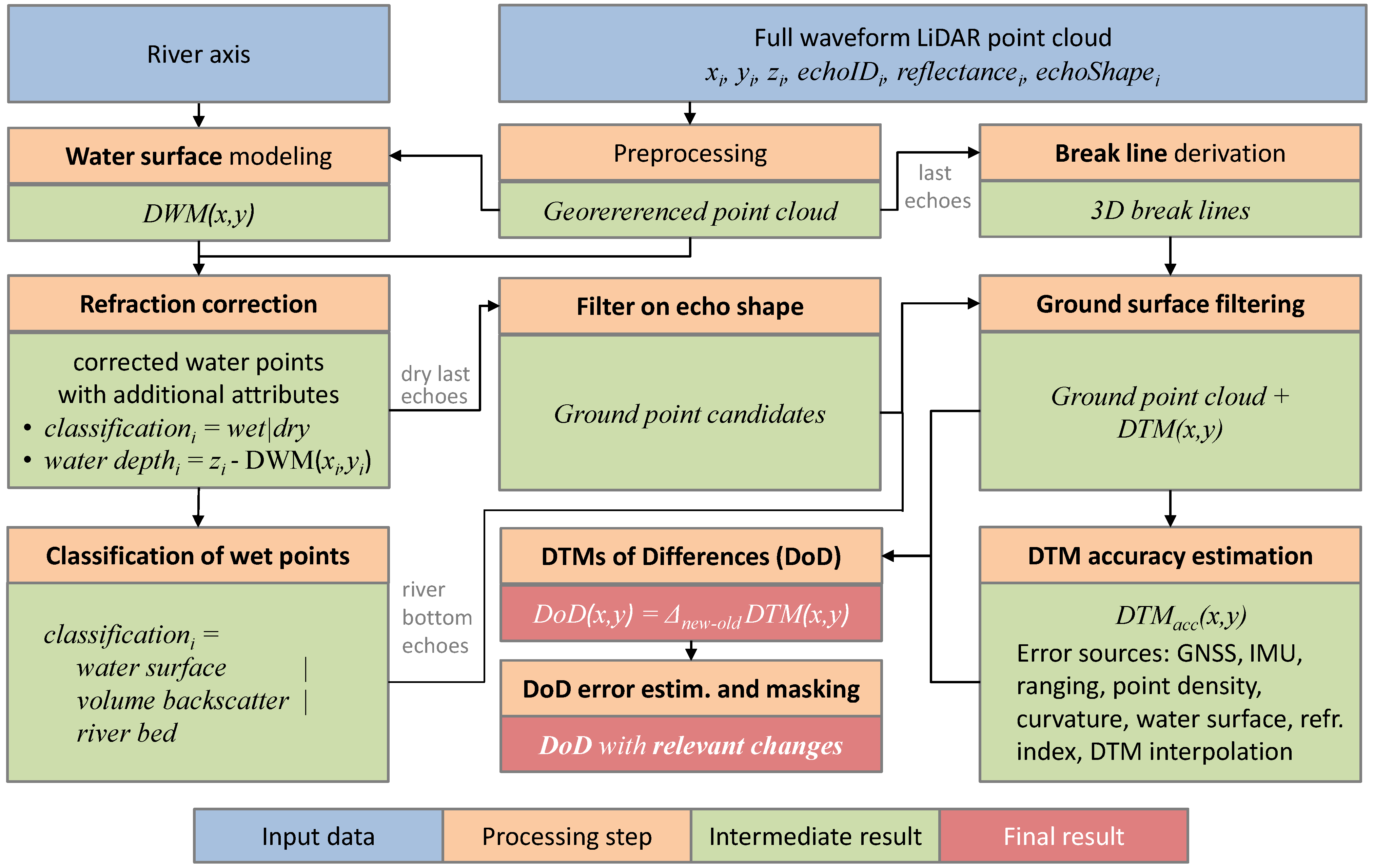
3. Methods
3.1. Modeling Terrain and River Surfaces

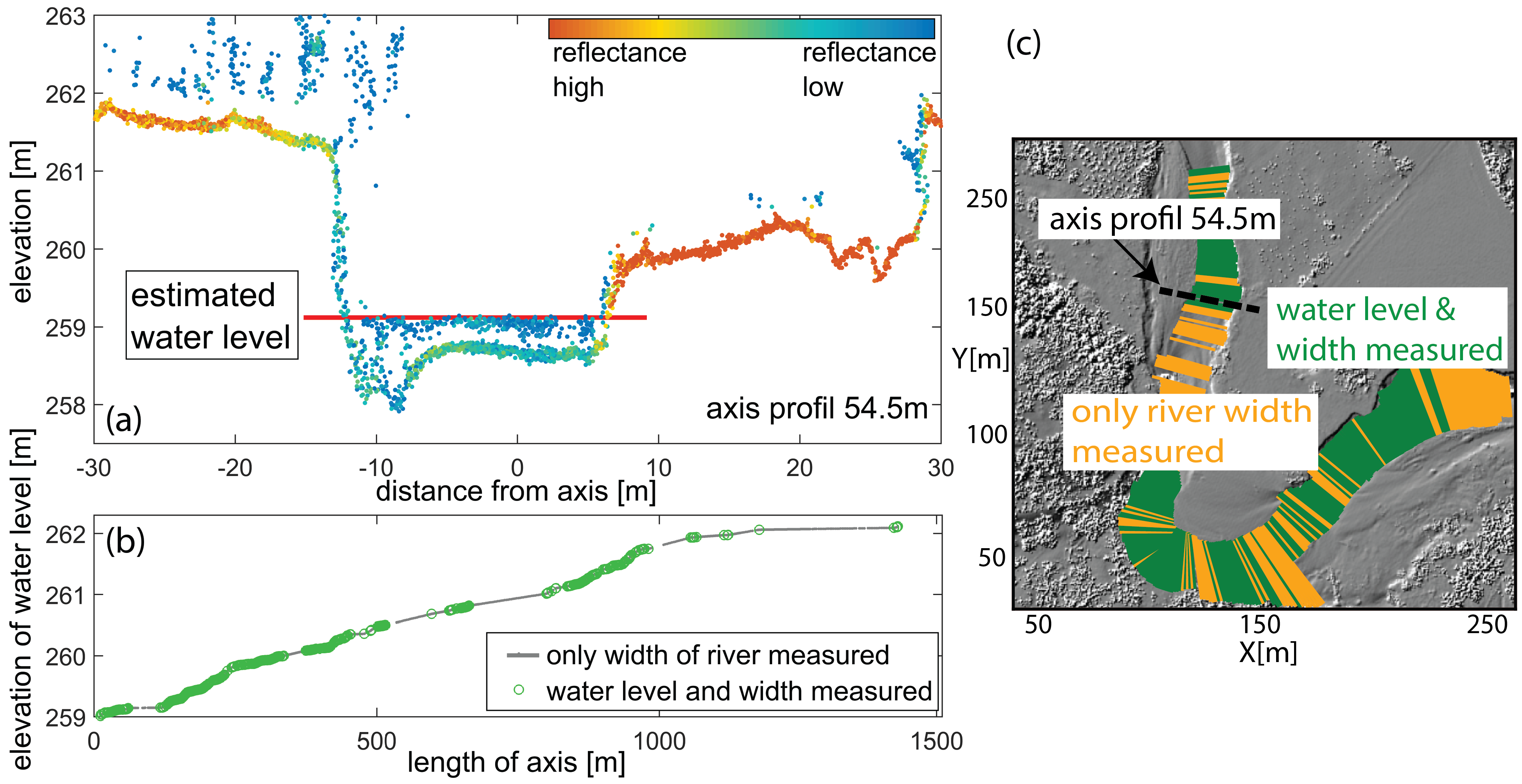
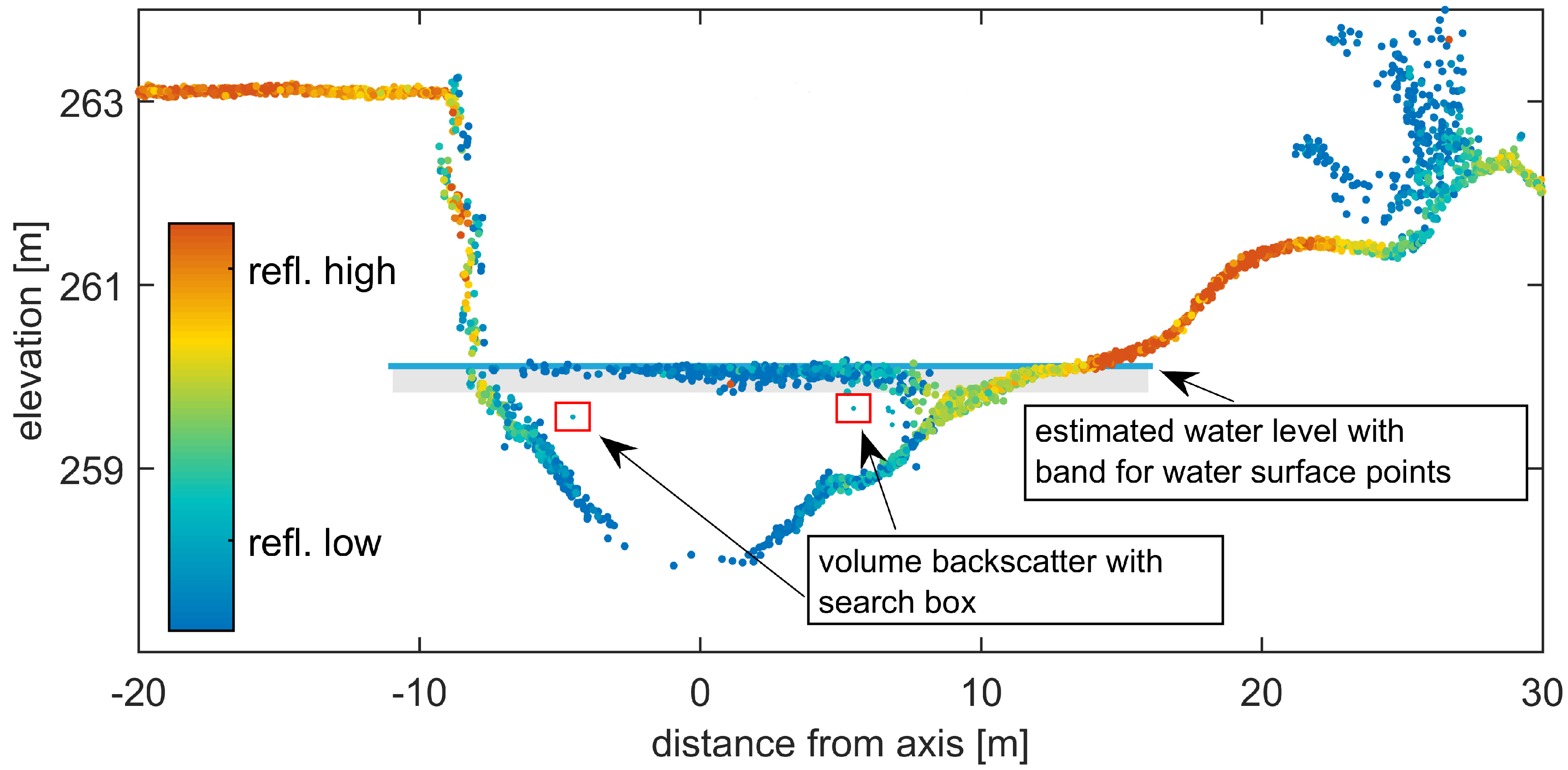
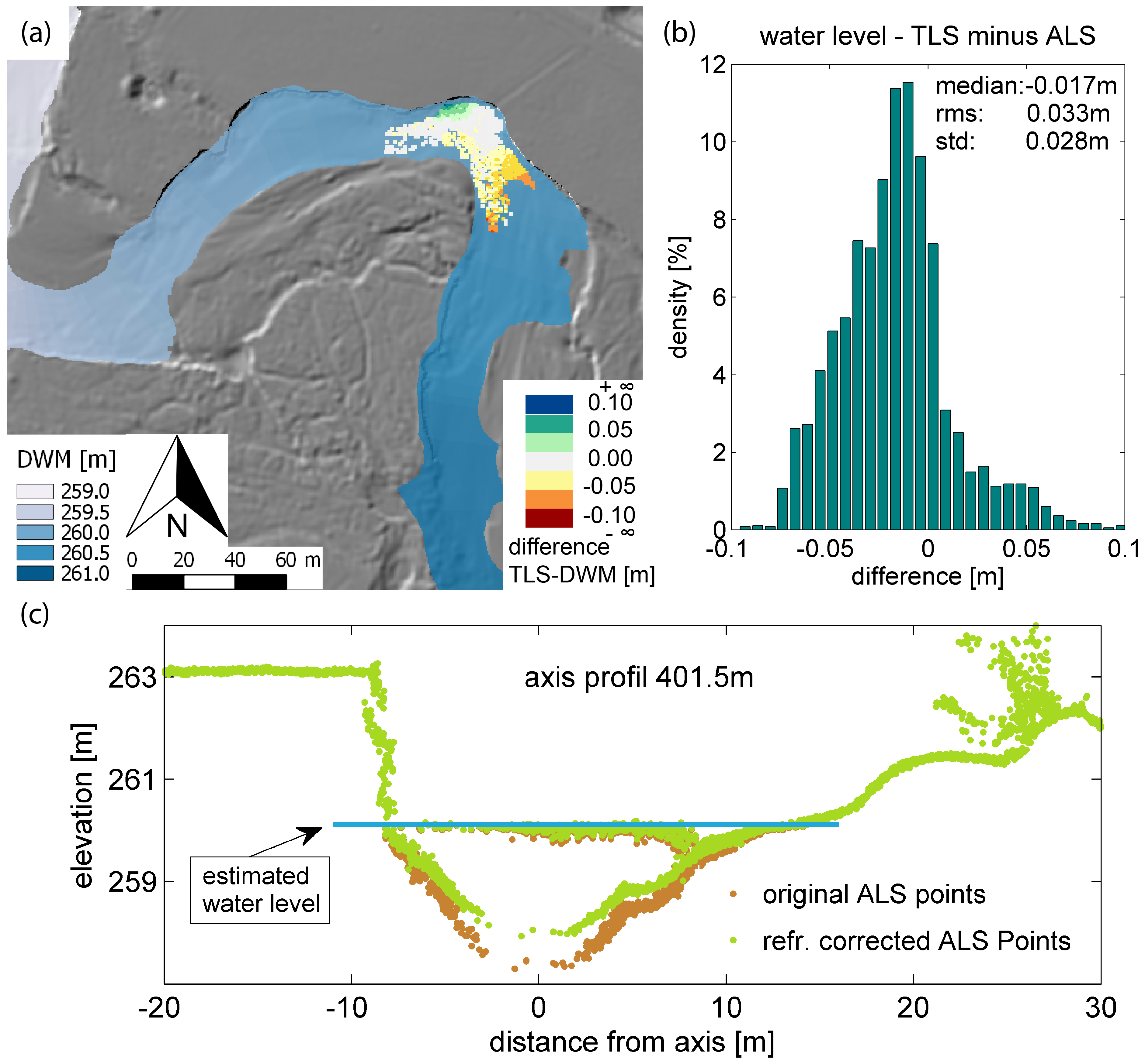
3.2. Water Surface Modeling

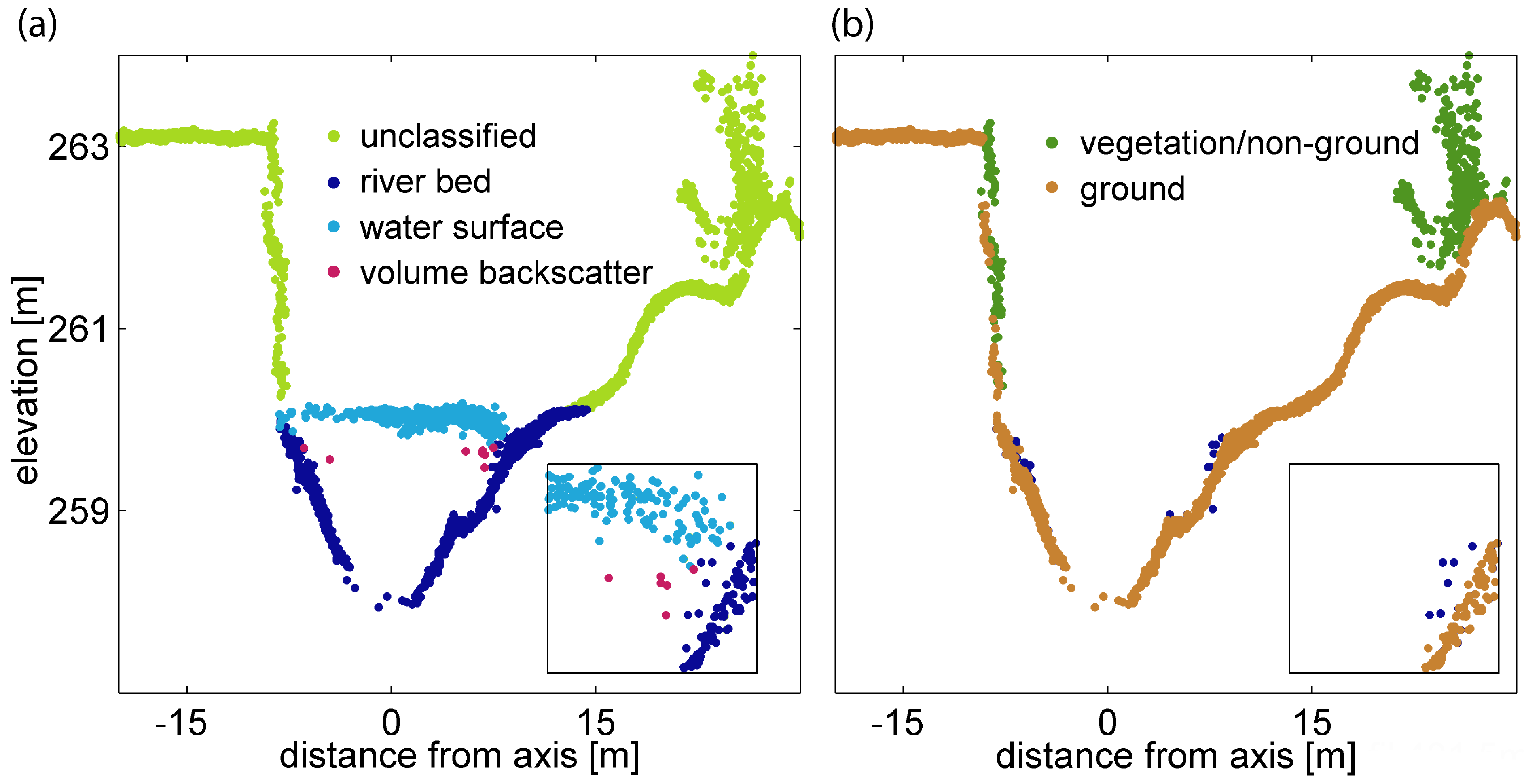
3.3. Water Body Classification

3.4. Terrain Modeling
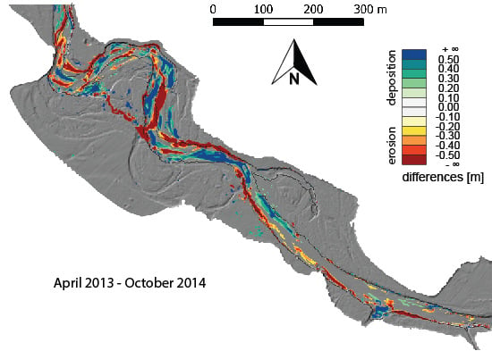
3.5. DEM of Differences
3.6. Habitat Modeling
4. Results and Discussion
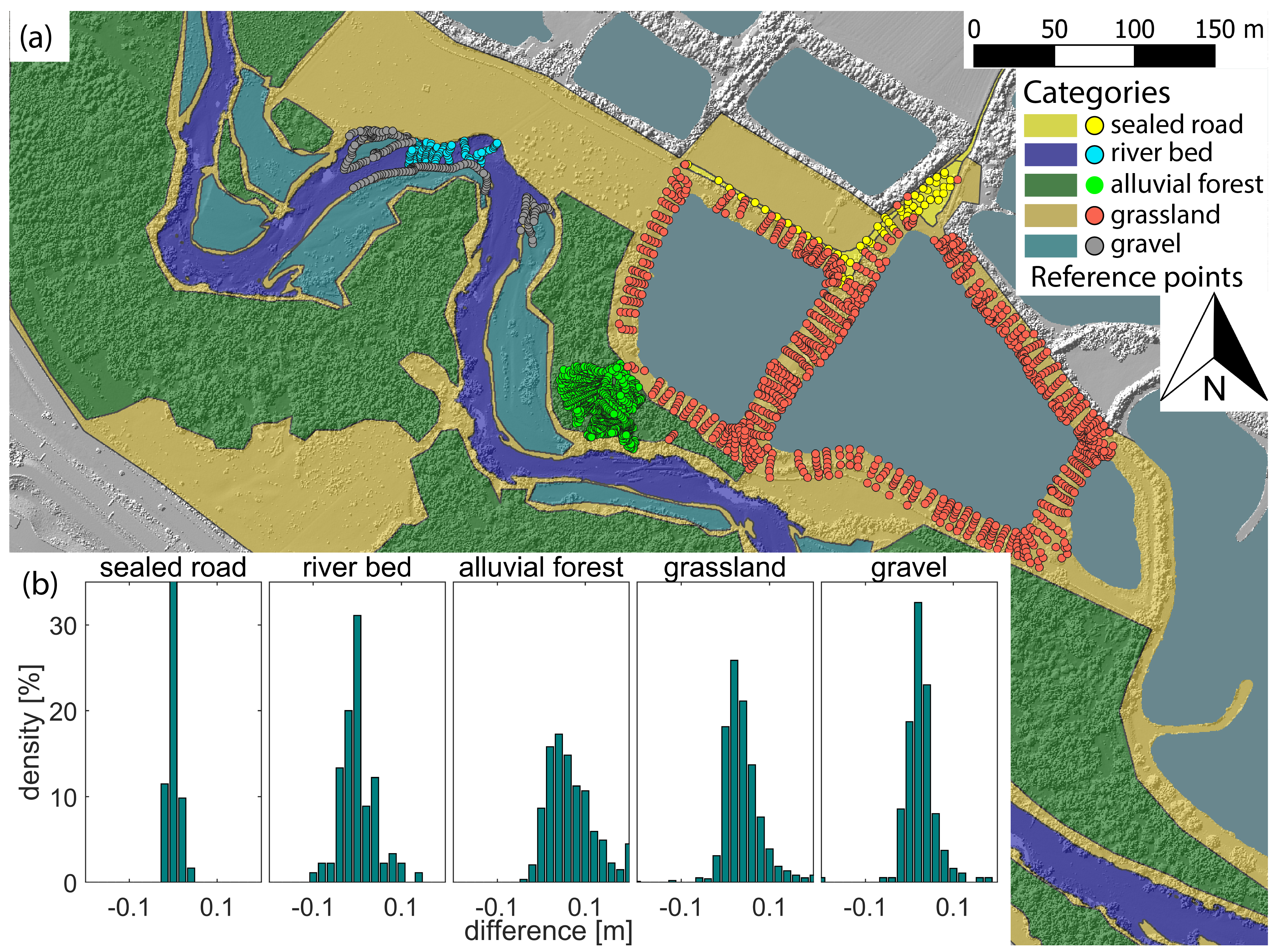
4.1. Point Cloud Accuracy Assessment
| Parameter | Sealed Road | River Bed | Alluvial Forest | Grassland | Gravel Bank |
|---|---|---|---|---|---|
| Mean [m] | 0.001 | 0.000 | 0.069 | 0.038 | 0.025 |
| Median [m] | 0.001 | –0.006 | 0.055 | 0.031 | 0.022 |
| Std.dev. [m] | 0.011 | 0.040 | 0.058 | 0.042 | 0.037 |
| sigmaMAD [m] | 0.007 | 0.025 | 0.050 | 0.031 | 0.022 |
| Surface roughness [m] | 0.000 | 0.024 | 0.050 | 0.030 | 0.021 |

4.2. Classification and Surface Modeling


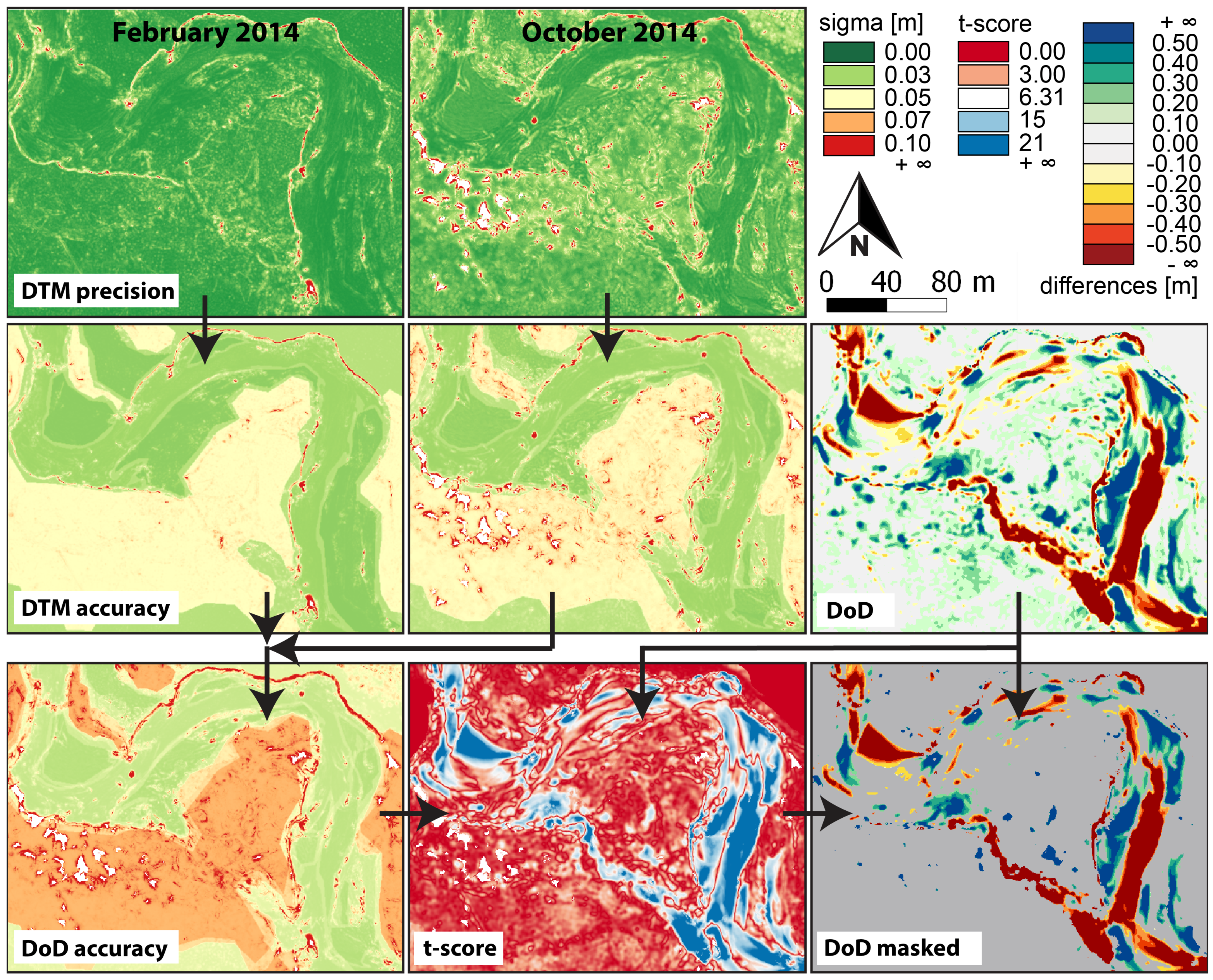
4.3. DTM Quality and DoD Masking

| Volumetric Change [m3] | Raw | Masked (95% Confidence Interval) | |||||
|---|---|---|---|---|---|---|---|
| Period | Change | MQ | HQ1 | MQ | HQ1 | Total | Sum |
| Apr13–Oct13 | deposition | 4.749 | 10.631 | 2.565 | 877 | 3.442 | 435 |
| erosion | –3.353 | –2.134 | –2.089 | –918 | –3.007 | ||
| Oct13–Feb14 | deposition | 1.548 | 1.307 | 554 | 175 | 729 | |
| erosion | –2.981 | –8.964 | –1.056 | –174 | –1.230 | –501 | |
| Apr13–Feb14 | deposition | 4.040 | 3.664 | 2.282 | 642 | 2.924 | |
| erosion | –4.078 | –2.823 | –2.562 | –885 | –3.447 | –523 | |
| Feb14–Oct14 | deposition | 5.793 | 10.634 | 4.161 | 1.006 | 5.167 | |
| erosion | –5.021 | –8.093 | –3.495 | –5.754 | –9.249 | –4.082 | |
| Apr13–Oct14 | deposition | 6.906 | 11.690 | 5.470 | 1.610 | 7.080 | |
| erosion | –6.171 | –8.308 | –4.527 | –5.958 | –10.485 | –3.405 | |
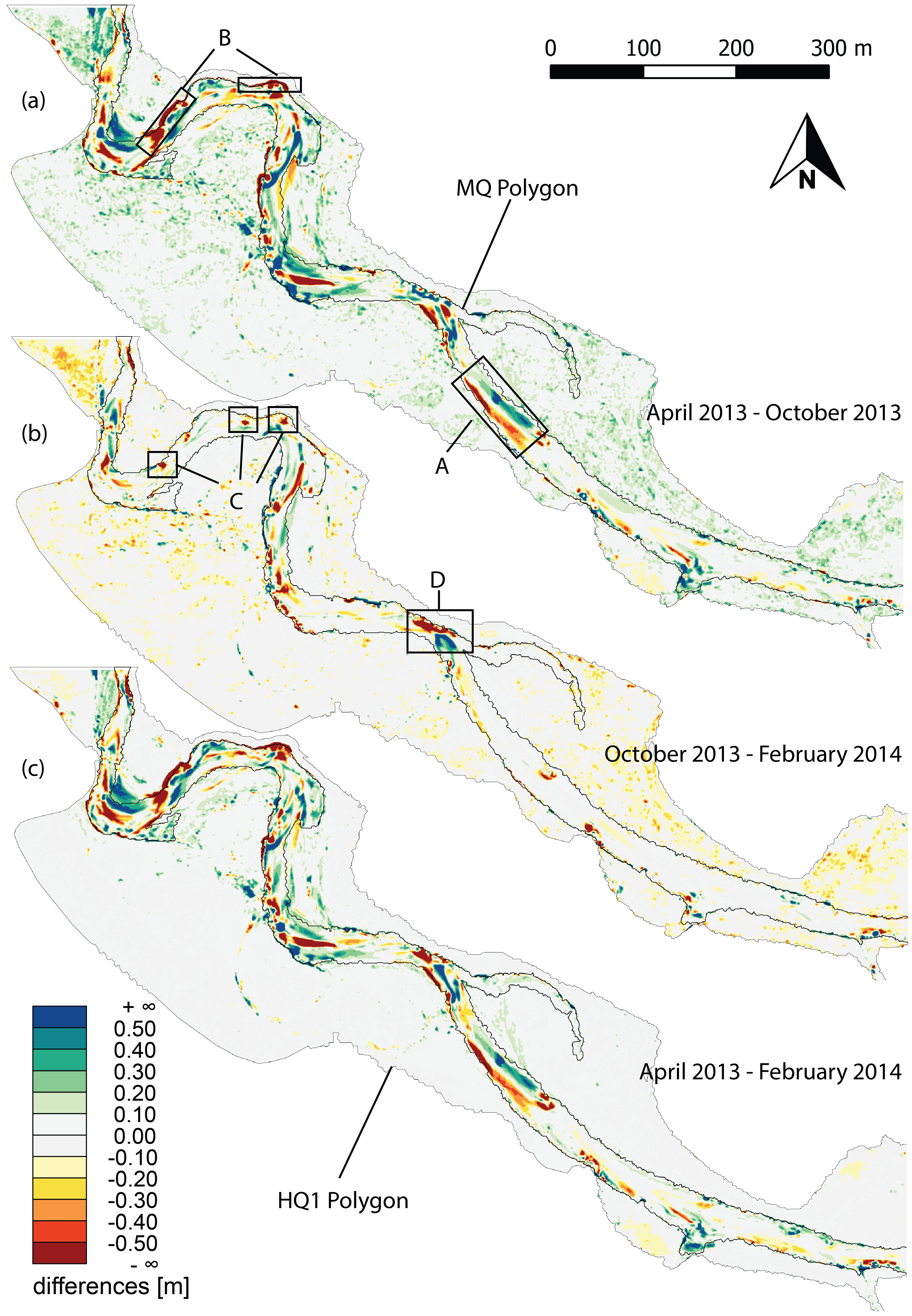
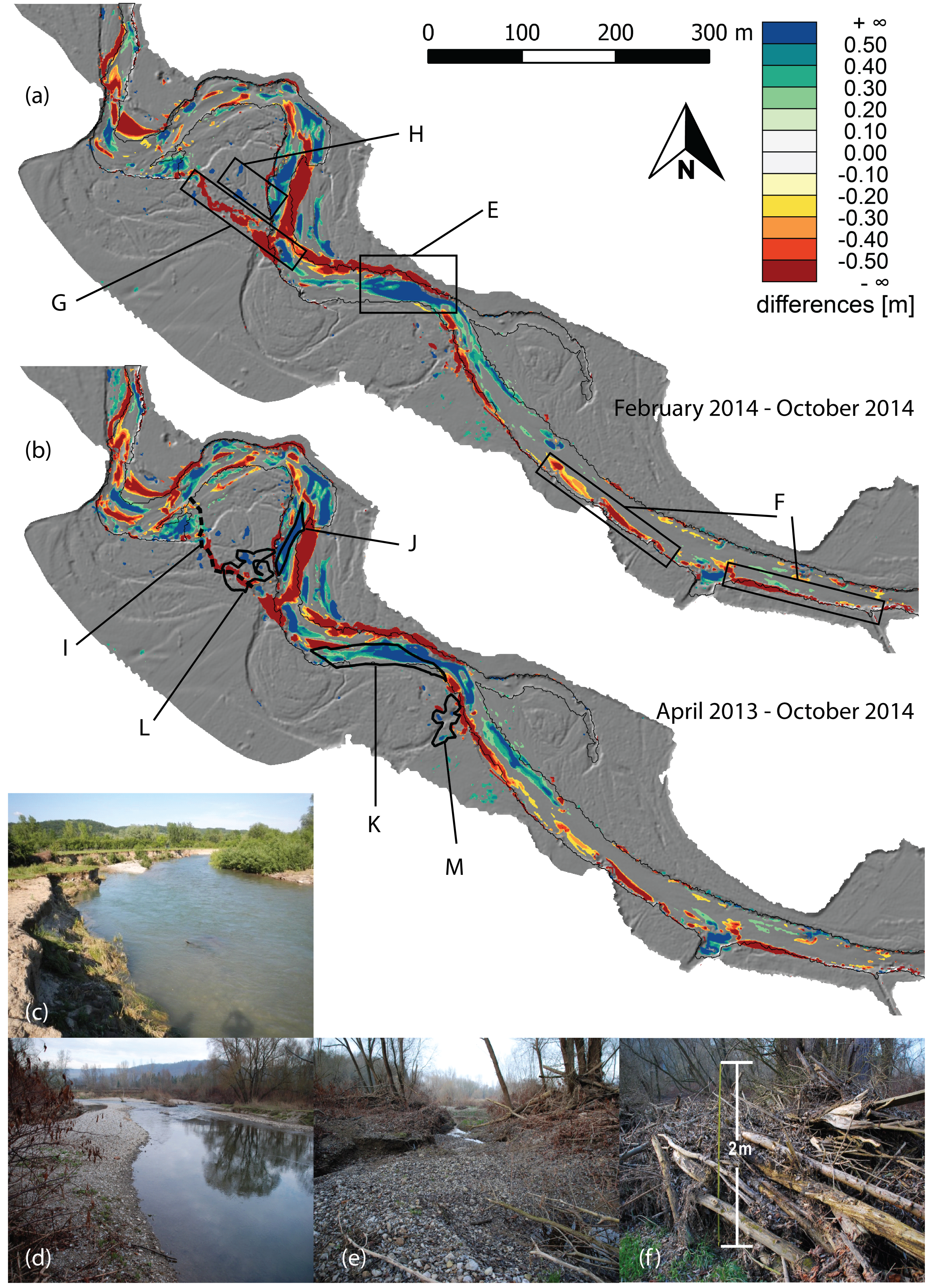
4.4. River Morphodynamics


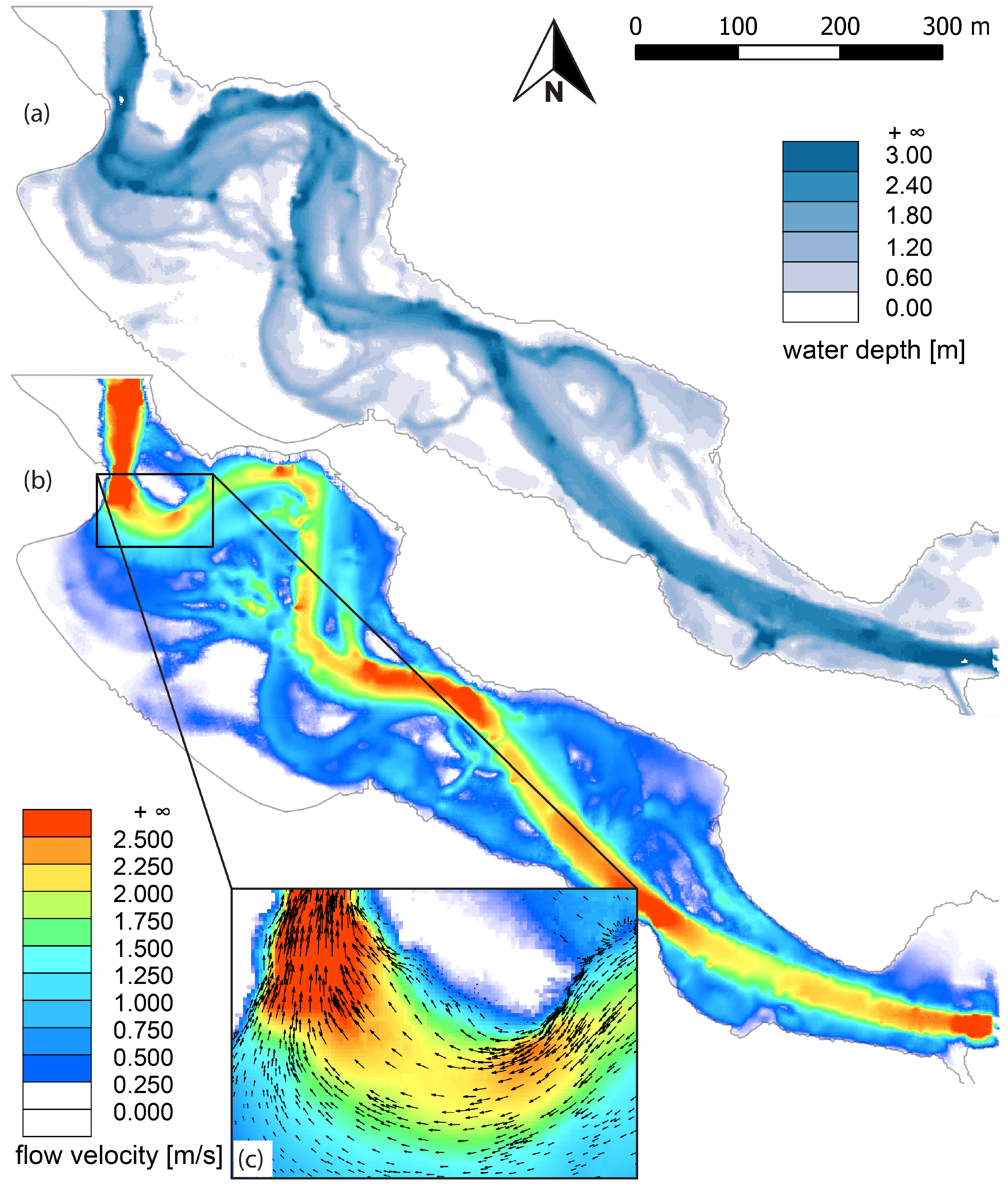
4.5. Flood Studies

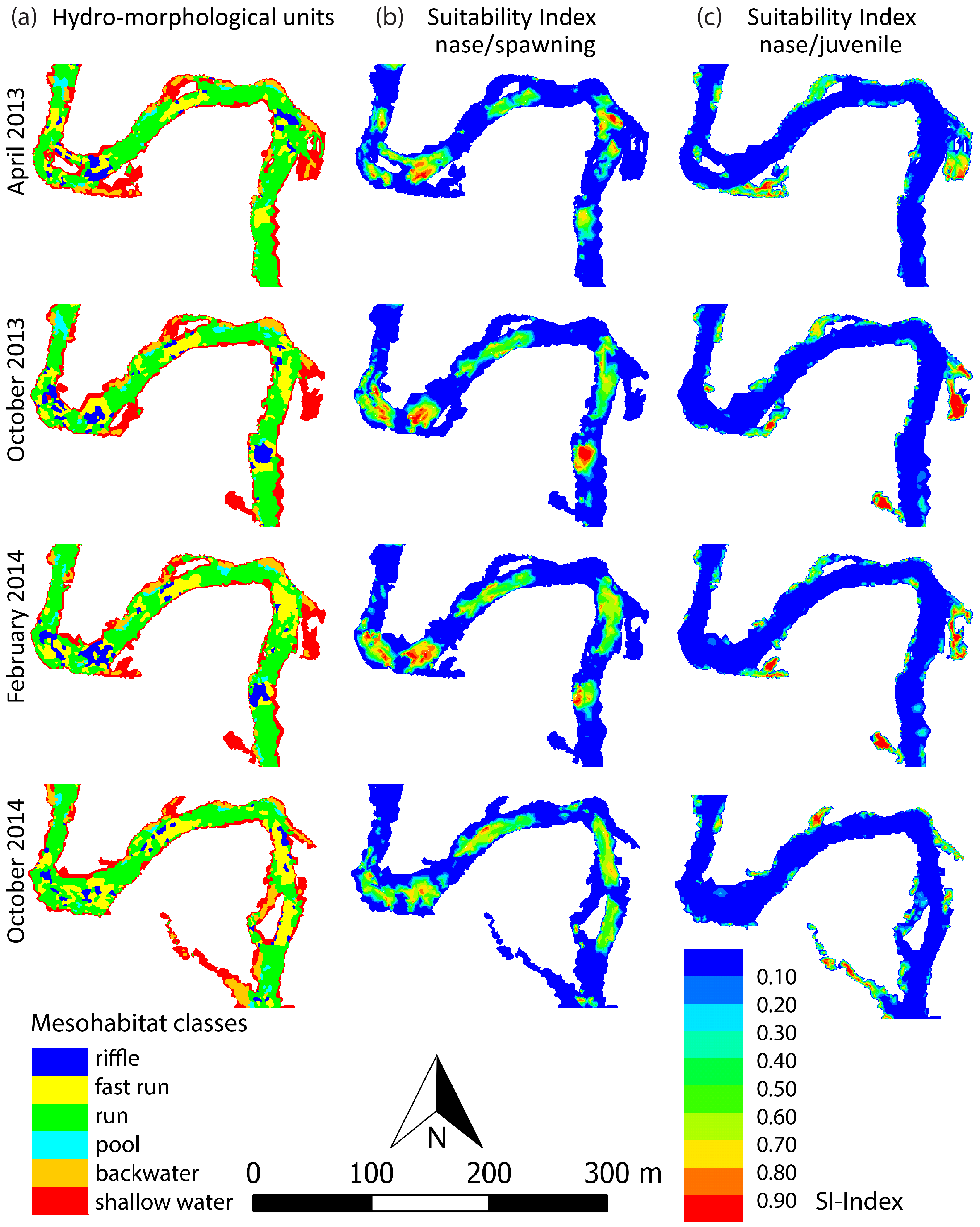
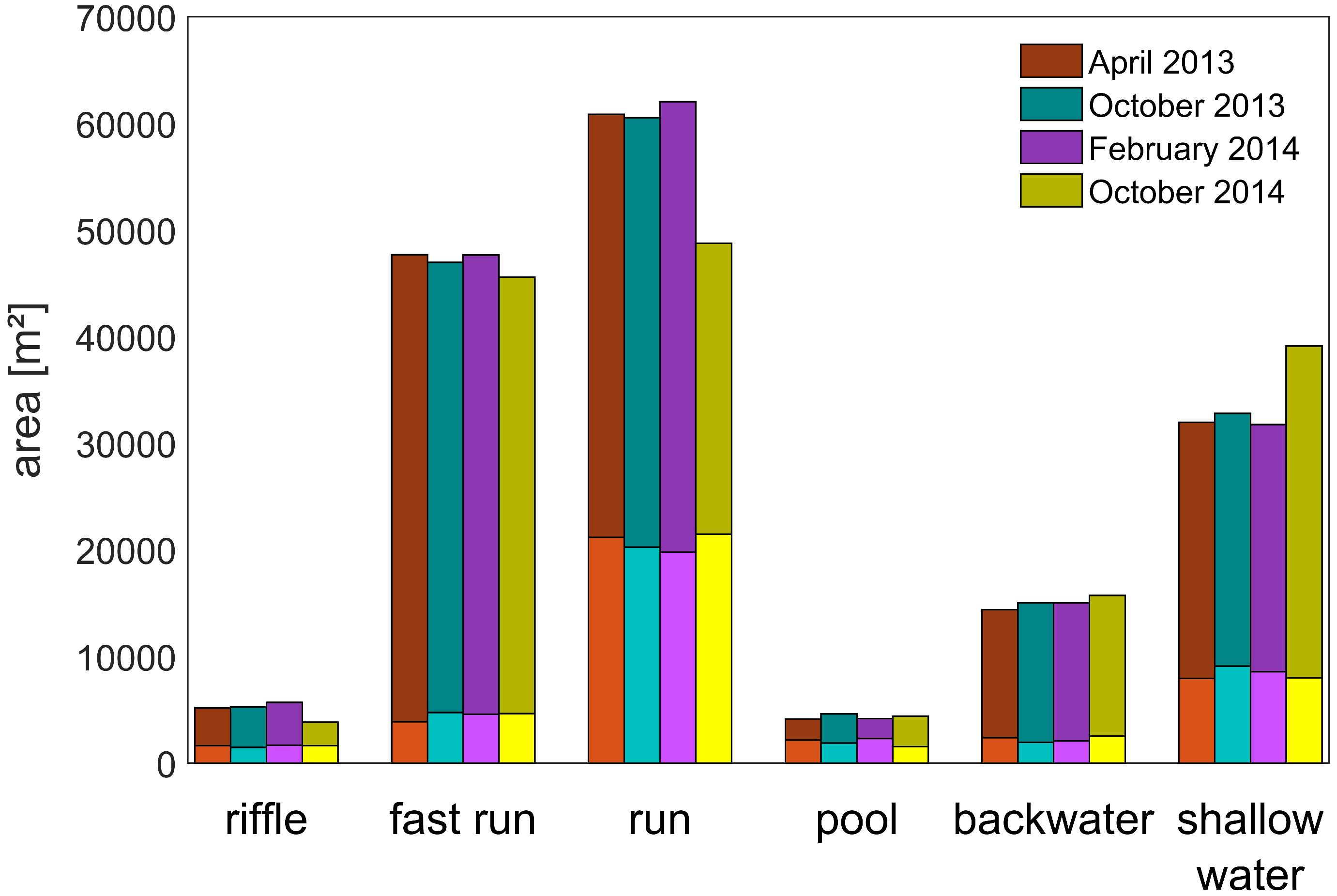
4.6. Habitats


5. Conclusions
Acknowledgments
Author Contributions
Conflicts of Interest
References
- Borre, J.V.; Paelinckx, D.; Mücher, C.A.; Kooistra, L.; Haest, B.; Blust, G.D.; Schmidt, A.M. Integrating remote sensing in Natura 2000 habitat monitoring: Prospects on the way forward. J. Nat. Conserv. 2011, 19, 116–125. [Google Scholar] [CrossRef]
- Spanhove, T.; Borre, J.V.; Delalieux, S.; Haest, B.; Paelinckx, D. Can remote sensing estimate fine-scale quality indicators of natural habitats? Ecol. Indic. 2012, 18, 403–412. [Google Scholar] [CrossRef]
- European Union. Council Directive 92/43/EEC on the Conservation of Natural Habitats and of Wild Fauna and Flora. Available online: http://www.planningni.gov.uk/downloads/draft_shadow_hra_july_2014.pdf (accessed on 15 January 2015).
- Corbane, C.; Lang, S.; Pipkins, K.; Alleaume, S.; Deshayes, M.; Millán, V.E.G.; Strasser, T.; Borre, J.V.; Toon, S.; Michael, F. Remote sensing for mapping natural habitats and their conservation status—New opportunities and challenges. Int. J. Appl. Earth Obs. Geoinf. 2015, 37, 7–16. [Google Scholar] [CrossRef]
- European Union. Directive 2000/60/EC of the European Parliament and of the Council of 23 October 2000 Establishing A Framework for Community Action the Field of Water Policy. Available online: http://www.ecolex.org/ecolex/ledge/view/RecordDetails;jsessionid=A130ECBA79C3616C3A61F6B4368B5997?id=LEX-FAOC023005&index=documents (accessed on 13 May 2015).
- European Union. Directive 2007/60/EC of the European Parliament and European Council of October 2007 on the Assessment and Management of Flood Risks. Available online: http://eur-lex.europa.eu/legal-content/EN/TXT/?uri=CELEX:32007L0060 (accessed on 13 May 2015).
- Wheaton, J.M.; Pasternack, G.B.; Merz, J.E. Use of habitat heterogeneity in salmonid spawning habitat rehabilitation design. In Proceedings of the Fifth IAHR International Symposium on Habitat Hydraulics, Madrid, Spain, 12–17 September 2004.
- Gard, M. Modeling changes in salmon spawning and rearing habitat associated with river channel restoration. Int. J. River Basin Manag. 2006, 4, 201–211. [Google Scholar] [CrossRef]
- Hauer, C.; Mandlburger, G.; Habersack, H. Hydraulically related hydro-morphological units: Description based on a new conceptual mesohabitat evaluation model (MEM) using LiDAR data as geometric input. River Res. Appl. 2009, 25, 29–47. [Google Scholar] [CrossRef]
- Kemp, J.L.; Harper, D.M.; Crosa, G.A. Use of “functional habitats” to link ecology with morphology and hydrology in river rehabilitation. Aquatic Conserv. Mar. Freshw. Ecosyst. 1999, 9, 159–178. [Google Scholar] [CrossRef]
- Wu, W.; Rodi, W.; Wenka, T. 3D numerical modeling of flow and sediment transport in open channels. J. Hydr. Eng. 2000, 126, 4–15. [Google Scholar] [CrossRef]
- Wheaton, J.M.; Brasington, J.; Darby, S.E.; Merz, J.; Pasternack, G.B.; Sear, D.; Vericat, D. Linking geomorphic changes to salmonid habitat at a scale relevant to fish. River Res. Appl. 2010, 26, 469–486. [Google Scholar] [CrossRef]
- Apel, H.; Aronica, G.; Kreibich, H.; Thieken, A. Flood risk analyses—How detailed do we need to be? Nat. Hazards 2009, 49, 79–98. [Google Scholar] [CrossRef]
- Olsen, J.; Beling, P.; Lambert, J.; Haimes, Y. Input-output economic evaluation of system of levees. J. Water Resour. Plan. Manag. 1998, 124, 237–245. [Google Scholar] [CrossRef]
- Hardmeyer, K.; Spencer, M.A. Using risk-Based analysis and geographic information systems to assess flooding problems in an urban watershed in Rhode Island. Environ. Manag. 2007, 39, 563–574. [Google Scholar] [CrossRef] [PubMed]
- Grünthal, G.; Thieken, A.; Schwarz, J.; Radtke, K.; Smolka, A.; Merz, B. Comparative risk assessments for the City of Cologne—Storms, floods, earthquakes. Nat. Hazards 2006, 38, 21–44. [Google Scholar] [CrossRef]
- Dutta, D.; Herath, S.; Musiake, K. An application of a flood risk analysis system for impact analysis of a flood control plan in a river basin. Hydrol. Process. 2006, 20, 1365–1384. [Google Scholar] [CrossRef]
- Mandlburger, G.; Hauer, C.; Höfle, B.; Habersack, H.; Pfeifer, N. Optimisation of Lidar derived terrain models for river flow modelling. Hydrol. Earth Syst. Sci. 2009, 13, 1453–1466. [Google Scholar] [CrossRef]
- Lee, Z.; Carder, K.L.; Mobley, C.D.; Steward, R.G.; Patch, J.S. Hyperspectral remote sensing for shallow waters. I. A semianalytical model. Appl. Optics 1998, 37, 6329–6338. [Google Scholar] [CrossRef]
- Marcus, W.; Legleiter, C.J.; Aspinall, R.J.; Boardman, J.W.; Crabtree, R.L. High spatial resolution hyperspectral mapping of in-stream habitats, depths, and woody debris in mountain streams. Geomorphology 2003, 55, 363–380. [Google Scholar] [CrossRef]
- Marcus, W.A.; Fonstad, M.A. Optical remote mapping of rivers at sub-meter resolutions and watershed extents. Earth Surf. Proc. Land. 2008, 33, 4–24. [Google Scholar] [CrossRef]
- Legleiter, C.J.; Roberts, D.A.; Lawrence, R.L. Spectrally based remote sensing of river bathymetry. Earth Surf. Proc. Land. 2009, 34, 1039–1059. [Google Scholar] [CrossRef]
- Lane, S.N.; Widdison, P.E.; Thomas, R.E.; Ashworth, P.J.; Best, J.L.; Lunt, I.A.; Sambrook Smith, G.H.; Simpson, C.J. Quantification of braided river channel change using archival digital image analysis. Earth Surf. Proc. Land. 2010, 35, 971–985. [Google Scholar] [CrossRef]
- Brando, V.; Dekker, A. Satellite hyperspectral remote sensing for estimating estuarine and coastal water quality. IEEE Trans. Geosci. Remote Sens. 2003, 41, 1378–1387. [Google Scholar] [CrossRef]
- Lindberg, E.; Olofsson, K.; Holmgren, J.; Olsson, H. Estimation of 3D vegetation structure from waveform and discrete return airborne laser scanning data. Remote Sens. Environ. 2011, 118, 151–161. [Google Scholar] [CrossRef]
- Van Leeuwen, M.; Nieuwenhuis, M. Retrieval of forest structural parameters using Lidar remote sensing. Eur. J. Forest Res. 2010, 129, 749–770. [Google Scholar] [CrossRef]
- Schneider, F.D.; Leiterer, R.; Morsdorf, F.; Gastellu-Etchegorry, J.P.; Lauret, N.; Pfeifer, N.; Schaepman, M.E. Simulating imaging spectrometer data: 3D forest modeling based on Lidar and in situ data. Remote Sens. Environ. 2014, 152, 235–250. [Google Scholar] [CrossRef]
- Pfeifer, N.; Mandlburger, G. Filtering and DTM generation. In Topographic Laser Ranging and Scanning: Principles and Processing; Shan, J., Toth, C.K., Eds.; CRC Press: Boca Raton, FL, USA, 2008; pp. 307–334. [Google Scholar]
- Otepka, J.; Ghuffar, S.; Waldhauser, C.; Hochreiter, R.; Pfeifer, N. Georeferenced point dlouds: A survey of features and point cloud management. ISPRS Int. J. Geoinf. 2013, 2, 1038–1065. [Google Scholar] [CrossRef]
- Guenther, G.C.; Cunningham, A.G.; Laroque, P.E.; Reid, D.J. Meeting the accuracy challenge in airborne Lidar bathymetry. In Proceedings of the 20th EARSeL Symposium: Workshop on Lidar Remote Sensing of Land and Sea, Dresden, Germany, 16–17 June 2000.
- Guenther, G.C.; LaRocque, P.E.; Lillycrop, W.J. Multiple surface channels in Scanning Hydrographic Operational Airborne Lidar Survey (SHOALS) airborne Lidar. Proc. SPIE 1994, 2258, 422–430. [Google Scholar]
- Mandlburger, G.; Pfennigbauer, M.; Pfeifer, N. Analyzing near water surface penetration in laser bathymetry—A case study at the River Pielach. In Proceedings of ISPRS Annals of the Photogrammetry, Remote Sensing and Spatial Information Sciences, Antalya, Turkey, 11–13 Novermber 2013.
- Lane, S.N.; Chandler, J.H. Editorial: The generation of high quality topographic data for hydrology and geomorphology: New data sources, new applications and new problems. Earth Surf. Proc. Land. 2003, 28, 229–230. [Google Scholar] [CrossRef]
- Lane, S.N. The use of digital terrain modelling in the understanding of dynamic river channel systems. In Landform Monitoring, Modelling and Analysis; Wiley: Hoboken, NJ, USA, 1998; pp. 311–342. [Google Scholar]
- Brockmann, H.; Mandlburger, G. Modelling a watercourse DTM based on airborne laser-scanner data—Using the example of the River Oder along the German/Polish Border. In Proceedings of OEEPE Workshop on Airborne Laserscanning and Interferometric SAR for Detailed Digital Terrain Models, Stockholm, Sweden, 1–3 March 2001.
- Brasington, J.; Rumsby, B.T.; McVey, R.A. Monitoring and modelling morphological change in a braided gravel-bed river using high resolution GPS-based survey. Earth Surf. Proc. Land. 2000, 25, 973–990. [Google Scholar] [CrossRef]
- Merz, J.E.; Pasternack, G.B.; Wheaton, J.M. Sediment budget for salmonid spawning habitat rehabilitation in a regulated river. Geomorphology 2006, 76, 207–228. [Google Scholar] [CrossRef]
- Heritage, G.; Hetherington, D. Towards a protocol for laser scanning in fluvial geomorphology. Earth Surf. Proc. Land. 2007, 32, 66–74. [Google Scholar] [CrossRef]
- Hodge, R.; Brasington, J.; Richards, K. Analysing laser-scanned digital terrain models of gravel bed surfaces: Linking morphology to sediment transport processes and hydraulics. Sedimentology 2009, 56, 2024–2043. [Google Scholar] [CrossRef]
- Notebaert, B.; Verstraeten, G.; Govers, G.; Poesen, J. Qualitative and quantitative applications of Lidar imagery in fluvial geomorphology. Earth Surf. Proc. Land. 2009, 34, 217–231. [Google Scholar] [CrossRef]
- Legleiter, C.J. Remote measurement of river morphology via fusion of Lidar topography and spectrally based bathymetry. Earth Surf. Proc. Land. 2012, 37, 499–518. [Google Scholar] [CrossRef]
- Williams, R.D.; Brasington, J.; Vericat, D.; Hicks, D.M. Hyperscale terrain modelling of braided rivers: Fusing mobile terrestrial laser scanning and optical bathymetric mapping. Earth Surf. Proc. Land. 2014, 39, 167–183. [Google Scholar] [CrossRef]
- Moretto, J.; Rigon, E.; Mao, L.; Delai, F.; Picco, L.; Lenzi, M. Short-term geomorphic analysis in a disturbed fluvial environment by fusion of Lidar, colour bathymetry and dGPS surveys. CATENA 2014, 122, 180–195. [Google Scholar] [CrossRef]
- Delai, F.; Moretto, J.; Picco, L.; Rigon, E.; Ravazzolo, D.; Lenzi, M. Analysis of morphological processes in a disturbed gravel-bed river (Piave River): Integration of LiDAR data and colour bathymetry. J. Civil Eng. Archit. 2014, 8, 639–648. [Google Scholar]
- Rennie, C.D. Mapping water and sediment flux distributions in Gravel-bed Rivers using ADCPs. In Gravel-Bed Rivers; John Wiley Sons Inc: Hoboken, NJ, USA, 2012; pp. 342–350. [Google Scholar]
- Wheaton, J.M.; Brasington, J.; Darby, S.E.; Sear, D.A. Accounting for uncertainty in DEMs from repeat topographic surveys: improved sediment budgets. Earth Surf. Proc. Land. 2010, 35, 136–156. [Google Scholar] [CrossRef]
- Zavalas, R.; Ierodiaconou, D.; Ryan, D.; Rattray, A.; Monk, J. Habitat classification of temperate marine macroalgal communities using bathymetric Lidar. Remote Sens. 2014, 6, 2154–2175. [Google Scholar] [CrossRef]
- Wedding, L.M.; Friedlander, A.M.; McGranaghan, M.; Yost, R.S.; Monaco, M.E. Using bathymetric Lidar to define nearshore benthic habitat complexity: Implications for management of reef fish assemblages in Hawaii. Remote Sens. Environ. 2008, 112, 4159–4165. [Google Scholar] [CrossRef]
- Grande, M.; Chust, G.; Fernandes, J.A.; Galparsoro, I. Assessment of the discrimination potential of bathymetric Lidar and multispectral imagery for intertidal and subtidal habitats. In Proceedings of the 33th International Symposium on Remote Sensing of Environment (ISRSE), Stresa, Italy, 12 February 2009.
- Aslaksen, M.; Parrish, C.E. New Topographic-Bathymetric Lidar Technology for Post-Sandy Mapping. In Proceedings of Canadian Hydrographic Conference, St. John’s, Canada, 14–17 April 2014.
- Niemeyer, J.; Soergel, U. Opportunities of Airborne Laser Bathymetry for the Monitoring of the Sea Bed on the Baltic Sea Coast. Int. Arch. Photogramm. Remote Sens. Spat. Inf. Sci. 2013, XL-7/W2, 179–184. [Google Scholar] [CrossRef]
- Hilldale, R. Using bathymetric Lidar and a 2D hydraulic model to identify aquatic river habitat. In Proceedings of the World Environmental and Water Resources Congress 2007, Tampa, FL, USA, 15–19 May 2007.
- Kinzel, P.J.; Legleiter, C.J.; Nelson, J.M. Mapping River Bathymetry With a Small Footprint Green LiDAR: Applications and Challenges. JAWRA J. Am. Water Resour. Assoc. 2013, 49, 183–204. [Google Scholar] [CrossRef]
- Hilldale, R.; Raff, D. Assessing the ability of airborne Lidar to map river bathymetry. Earth Surf. Proc. Land. 2008, 33, 773–783. [Google Scholar] [CrossRef]
- Fernandez-Diaz, J.; Glennie, C.; Carter, W.; Shrestha, R.; Sartori, M.; Singhania, A.; Legleiter, C.; Overstreet, B. Early Results of Simultaneous Terrain and Shallow Water Bathymetry Mapping Using a Single-Wavelength Airborne LiDAR Sensor. IEEE J. Sel. Top. Appl. Earth Obs. Remote Sens. 2014, 7, 623–635. [Google Scholar] [CrossRef]
- McKean, J.; Tonina, D.; Bohn, C.; Wright, C. Effects of bathymetric lidar errors on flow properties predicted with a multi-dimensional hydraulic model. J. Geophys. Res.: Earth Surf. 2014, 119, 644–664. [Google Scholar] [CrossRef]
- Melcher, A.H.; Schmutz, S. The importance of structural features for spawning habitat of nase Chondrostoma nasus (L.) and barbel Barbus barbus (L.) in a pre-Alpine river. River Syst. 2010, 19, 33–42. [Google Scholar] [CrossRef]
- Montgomery, D.R.; Buffington, J.M. Channel reach morphology in mountain drainage basins. GSA Bull. 1997, 109, 596–611. [Google Scholar] [CrossRef]
- Zitek, A.; Schmutz, S.; Jungwirth, M. Assessing the efficiency of connectivity measures with regard to the EU-Water Framework Directive in a Danube-tributary system. Hydrobiologia 2008, 609, 139–161. [Google Scholar] [CrossRef]
- Zitek, A.; Schmutz, S. Efficiency of restoration measures in a fragmented Danube/tributary network. In Proceedings of the fifth IAHR International Symposium on Habitat Hydraulics, Madrid, Spain, 12–17 September 2004.
- Riegl LMS. VQ-820-G Datasheet. 2015. Available online: http://www.riegl.com/uploads/tx_pxpriegldownloads/DataSheet_VQ-820-G_2014-09-19.pdf (accessed on 13 May 2015).
- Riegl LMS. LAS Extrabytes Implementation in RIEGL Software. 2015. Available online: http://www.riegl.co.at/uploads/tx_pxpriegldownloads/Whitepaper_-_LAS_extrabytes_implementation_in_Riegl_software_01.pdf (accessed on 13 May 2015).
- Zhang, Y.; Shen, X. Direct georeferencing of airborne LiDAR data in national coordinates. ISPRS J. Photogramm. Remote Sens. 2013, 84, 43–51. [Google Scholar] [CrossRef]
- Skaloud, J.; Lichti, D. Rigorous approach to boresight self-calibration in airborne laser scanning. ISPRS J. Photogramm. Remote Sens. 2006, 61, 47–59. [Google Scholar] [CrossRef]
- Kager, H. Discrepancies between overlapping laser scanning strips—Simultaneous fitting of aerial laser scanner strips. Int. Arch. Photogramm. Remote Sens. Spat. Inf. Sci. 2004, XXXV, 555–560. [Google Scholar]
- Ressl, C.; Kager, H.; Mandlburger, G. Quality checking of ALS projects using statistics of strip differences. Int. Arch. Photogramm. Remote Sens. Spat. Inf. Sci. 2008, XXXVII, 253–260. [Google Scholar]
- Riegl LMS. RiProcess Datasheet. 2015. Available online: http://www.riegl.co.at/products/software-packages/riprocess/ (accessed on 13 May 2015).
- Pfeifer, N.; Mandlburger, G.; Otepka, J.; Karel, W. OPALS—A framework for Airborne Laser Scanning data analysis. Comput. Environ. Urban Syst. 2014, 45, 125–136. [Google Scholar] [CrossRef]
- Kraus, K.; Karel, W.; Briese, C.; Mandlburger, G. Local accuracy measures for digital terrain models. The Photogramm. Rec. 2006, 21, 342–354. [Google Scholar] [CrossRef]
- Nujic, M. Praktischer Einsatz Eines Hochgenauen Verfahrens für Die Berechnung Von Tiefengemittelten Strömungen. Ph.D. Thesis, Universität der Bundeswehr München, Munich, Germany, 1999. [Google Scholar]
- Vetter, M.; Höfle, B.; Mandlburger, G.; Rutzinger, M. Estimating changes of riverine landscapes and riverbeds by using airborne Lidar data and river cross-sections. Zeitschrift für Geomorph. Suppl. Issues 2011, 55, 51–65. [Google Scholar] [CrossRef]
- Smith, M.; Vericat, D.; Gibbins, C. Through-water terrestrial laser scanning of gravel beds at the patch scale. Earth Surf. Proc. Land. 2012, 37, 411–421. [Google Scholar] [CrossRef]
- Wernand, M.R. On the history of the Secchi disc. J. Eur. Opt. Soc. 2010, 5. [Google Scholar] [CrossRef]
- Briese, C.; Pfennigbauer, M.; Lehner, H.; Ullrich, A.; Wagner, W.; Pfeifer, N. Radiometric calibration of multi-wavelength airborne laser scanning data. ISPRS Ann. Photogramm. Remote Sens. Spatial Inf. Sci. 2012. [Google Scholar] [CrossRef]
- Sithole, G.; Vosselman, G. Experimental comparison of filtering algorithms for bare-earth extraction from airborne laser scanning point clouds. ISPRS J. Photogramm. Remote Sens. 2004, 59, 85–101. [Google Scholar] [CrossRef]
- Korzeniowska, K.; Pfeifer, N.; Mandlburger, G.; Lugmayr, A. Experimental evaluation of ALS point cloud ground extraction tools over different terrain slope and land-cover types. Int. J. Remote Sens. 2014, 35, 4673–4697. [Google Scholar] [CrossRef]
- Briese, C.; Mandlburger, G.; Ressl, C. Automatic break line determination for the generation of a DTM along the river Main. Int. Arch. Photogramm. Remote Sens. Spat. Inf. Sci. 2009, XXXVIII, 236–241. [Google Scholar]
- Doneus, M.; Briese, C.; Fera, M.; Janner, M. Archaeological prospection of forested areas using full-waveform airborne laser scanning. J. Archaeol. Sci. 2008, 35, 882–893. [Google Scholar] [CrossRef]
- Pfennigbauer, M.; Wolf, C.; Weinkopf, J.; Ullrich, A. Online waveform processing for demanding target situations. Proc. SPIE 2014. [Google Scholar] [CrossRef]
- Kraus, K.; Pfeifer, N. Determination of terrain models in sooded areas with airborne laser scanner data. ISPRS J. Photogramm. Remote Sens. 1998, 53, 193–203. [Google Scholar] [CrossRef]
- Pfeifer, N.; Stadler, P.; Briese, C. Derivation of digital terrain models in the SCOP++ environment. In Proceedings of OEEPE Workshop on Airborne Laserscanning and Interferometric SAR for Detailed Digital Terrain Models, Stockholm, Sweden, 1–3 March 2001.
- Kraus, K. Photogrammetry—Geometry from Images and Laser Scans, 2 ed.; Walter de Gruyter: Berlin, Germany, 2007. [Google Scholar]
- Brasington, J.; Langham, J.; Rumsby, B. Methodological sensitivity of morphometric estimates of coarse fluvial sediment transport. Geomorphology 2003, 53, 299–316. [Google Scholar] [CrossRef]
- Pironneau, O. Finite Element Methods for Fluids; John Wiley & Sons, Ltd: Paris, France, 1989; p. 208. [Google Scholar]
- Hauer, C.; Unfer, G.; Tritthart, M.; Formann, E.; Habersack, H. Variability of mesohabitat characteristics in riffle-pool reaches: testing an integrative evaluation concept (FGC) for MEM-application. River Res. Appl. 2011, 27, 403–430. [Google Scholar] [CrossRef]
- Hyyppä, H.; Yu, X.; Hyyppä, J.; Kaartinen, H.; Honkavaara, E.; Rönnholm, P. Factors affecting the quality of DTM generation in forested areas. Int. Arch. Photogramm. Remote Sens. Spat. Inf. Sci. 2005, XXXVI, 85–90. [Google Scholar]
- Turowski, J.M.; Badoux, A.; Rickenmann, D. Start and end of bedload transport in gravel-bed streams. Geophys. Res. Lett. 2011, 38. [Google Scholar] [CrossRef]
- Hauer, C.; Habersack, H. Morphodynamics of a 1000-year flood in the Kamp River, Austria, and impacts on floodplain morphology. Earth Surf. Proc. Land. 2009, 34, 654–682. [Google Scholar] [CrossRef]
- Tockner, K.; Malard, F.; Ward, J.V. An extension of the flood pulse concept. Hydrol. Process. 2000, 14, 2861–2883. [Google Scholar] [CrossRef]
- Railsback, S.F.; Stauffer, H.B.; Harvey, B.C. What can habitat preference models tell us? Tests using a virtual trout population. Ecol. Appl. 2003, 13, 1580–1594. [Google Scholar] [CrossRef]
- Manly, B.; McDonald, L.; Thomas, T.; Erickson, W. Resource Selection by Animals, 2 ed.; Kluwer Academic Publishers: Boston, MA, USA, 2002. [Google Scholar]
- Rosenfeld, J. Assessing the Habitat Requirements of Stream Fishes: An Overview and Evaluation of Different Approaches. Trans. Am. Fish. Soc. 2003, 132, 953–968. [Google Scholar] [CrossRef]
- Frissell, C.A.; Liss, W.J.; Warren, C.E.; Hurley, M.D. A hierarchical framework for stream habitat classification: Viewing streams in a watershed context. Environ. Manag. 1986, 10, 199–214. [Google Scholar] [CrossRef]
- Rossi, R.E.; J.Mulla, D.; Journel, A.G.; Franz, E.H. Geostatistical tools for modeling and interpreting ecological spatial dependence. Ecol. Monogr. 1992, 62, 277–314. [Google Scholar] [CrossRef]
- Naiman, A.J.; D. G. Lonzarich, T.J.B.; Ralph, S.C. General principles of classification and the assessment of conservation potential in rivers. In River Conservation and Management; John Wiley and Sons: Chichester, UK, 1992; pp. 93–123. [Google Scholar]
- Horne, J.K.; Schneider, D.C. Spatial Variance in Ecology. Oikos 1995, 74, 18–26. [Google Scholar] [CrossRef]
- Bult, T.P.; Haedrich, R.L.; Schneider, D.C. New technique describing spatial scaling and habitat selection in riverine habitats. Reg. Rivers Res. Manag. 1998, 14, 107–118. [Google Scholar] [CrossRef]
- Hawkins, C.P.; Kershner, J.L.; Bisson, P.A.; Bryant, M.D.; Decker, L.M.; Gregory, S.V.; McCullough, D.A.; Overton, C.K.; Reeves, G.H.; Steedman, R.J.; Young, M.K. A hierarchical approach to classifying stream habitat features. Fisheries 1993, 18, 3–12. [Google Scholar] [CrossRef]
- Habersack, H. The river-scaling concept (RSC): a basis for ecological assessments. Hydrobiologia 2000, 422–423, 49–60. [Google Scholar] [CrossRef]
- Bovee, K.D. Development and Evaluation of Habitat Suitability Criteria for Use in the Instream Flow Incremental Methodology; Technical Report Instream Flow Information Paper Nr. 21 FWS/OBS-86/7; USDI Fish and Wildlife Service: Washington, DC, USA, 1986. [Google Scholar]
- Hauer, C.; Unfer, G.; Holzapfel, P.; Haimann, M.; Habersack, H. Impact of channel bar form and grain size variability on estimated stranding risk of juvenile brown trout during hydropeaking. Earth Surf. Proc. Land. 2014, 39, 1622–1641. [Google Scholar] [CrossRef]
© 2015 by the authors; licensee MDPI, Basel, Switzerland. This article is an open access article distributed under the terms and conditions of the Creative Commons Attribution license (http://creativecommons.org/licenses/by/4.0/).
Share and Cite
Mandlburger, G.; Hauer, C.; Wieser, M.; Pfeifer, N. Topo-Bathymetric LiDAR for Monitoring River Morphodynamics and Instream Habitats—A Case Study at the Pielach River. Remote Sens. 2015, 7, 6160-6195. https://0-doi-org.brum.beds.ac.uk/10.3390/rs70506160
Mandlburger G, Hauer C, Wieser M, Pfeifer N. Topo-Bathymetric LiDAR for Monitoring River Morphodynamics and Instream Habitats—A Case Study at the Pielach River. Remote Sensing. 2015; 7(5):6160-6195. https://0-doi-org.brum.beds.ac.uk/10.3390/rs70506160
Chicago/Turabian StyleMandlburger, Gottfried, Christoph Hauer, Martin Wieser, and Norbert Pfeifer. 2015. "Topo-Bathymetric LiDAR for Monitoring River Morphodynamics and Instream Habitats—A Case Study at the Pielach River" Remote Sensing 7, no. 5: 6160-6195. https://0-doi-org.brum.beds.ac.uk/10.3390/rs70506160