
Remote Sensing Based Spatial Statistics to Document Tropical Rainforest Transition Pathways


Abstract
:
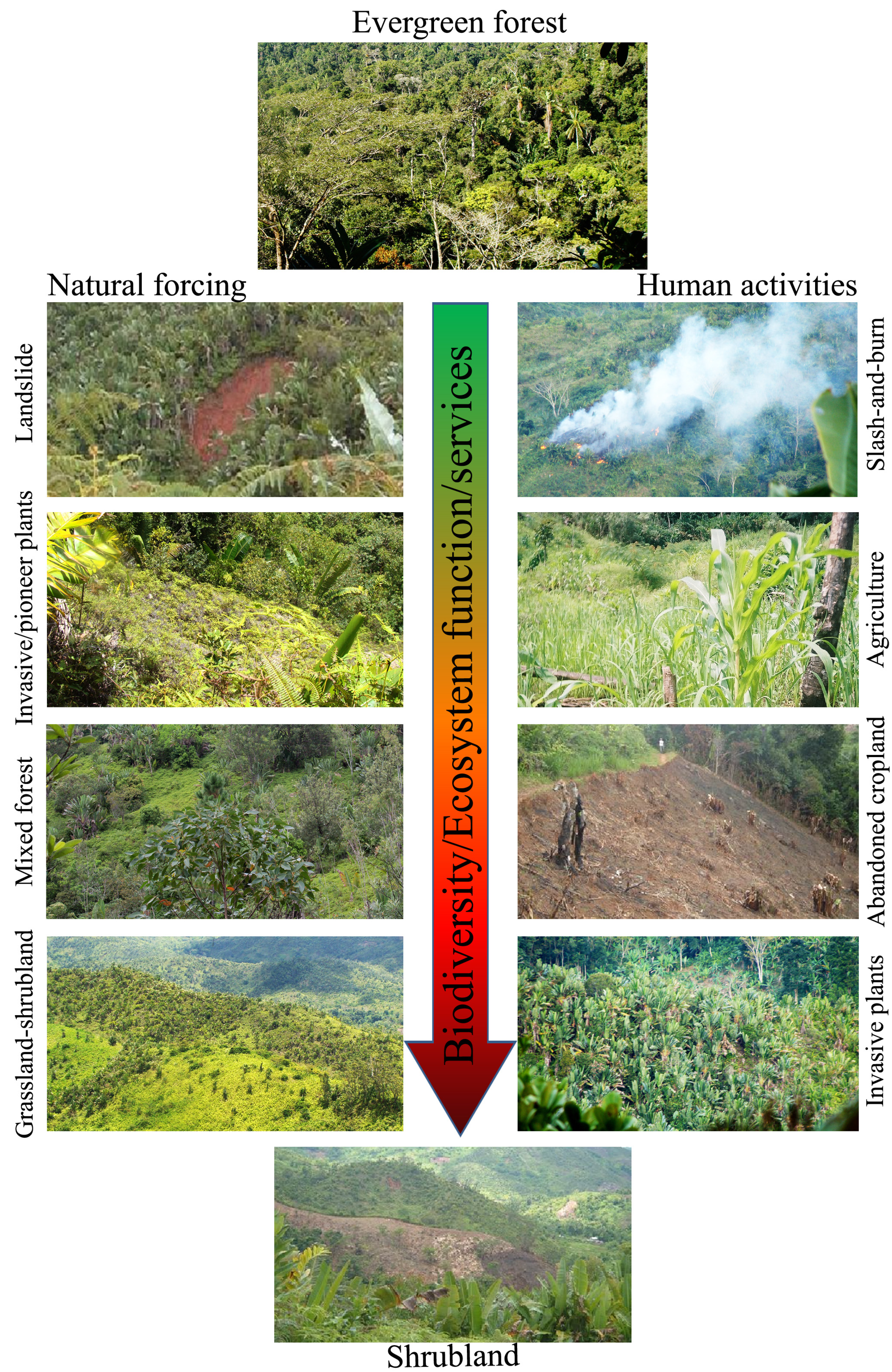
1. Introduction
2. Study Area and Data
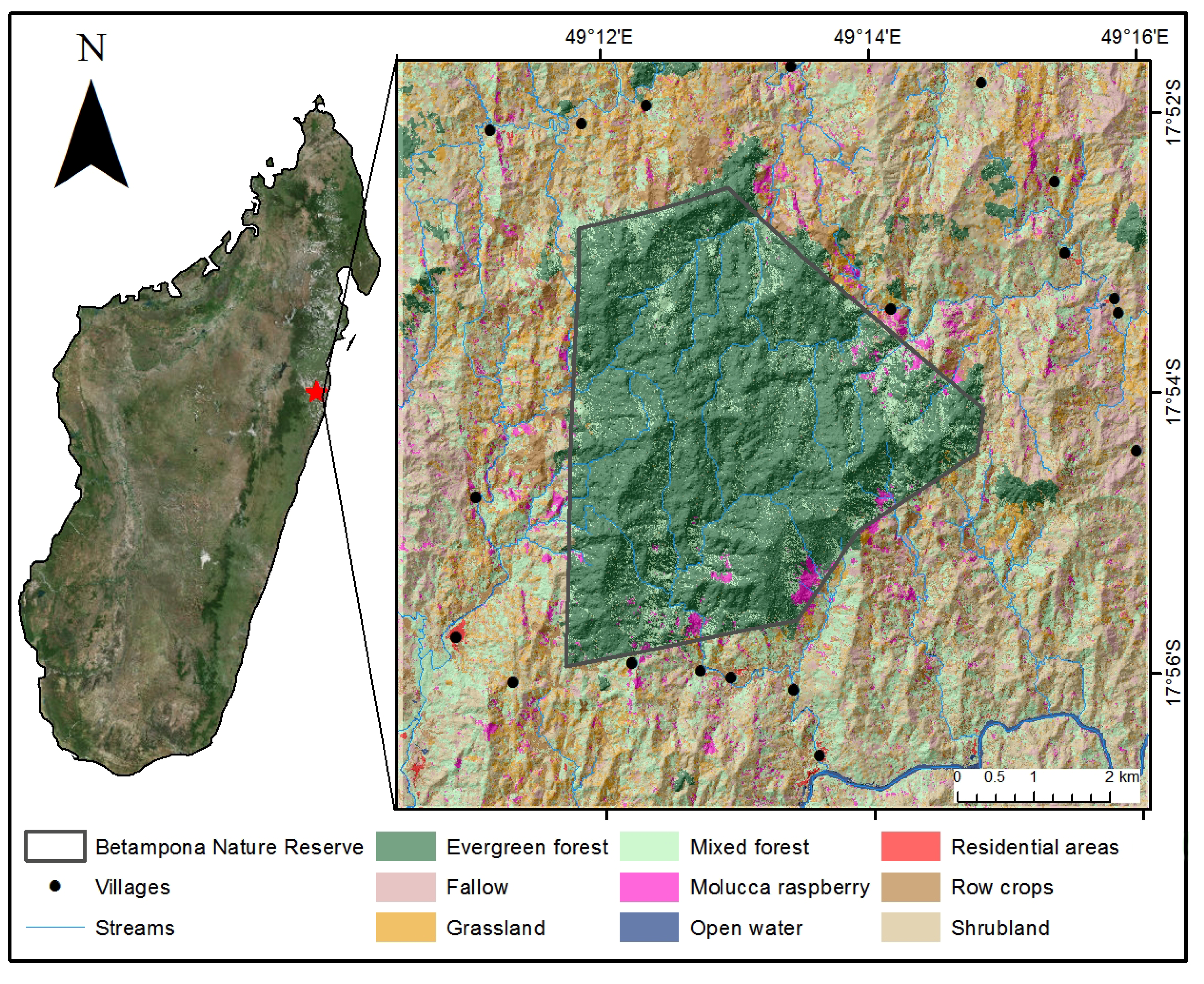
2.1. Study Site

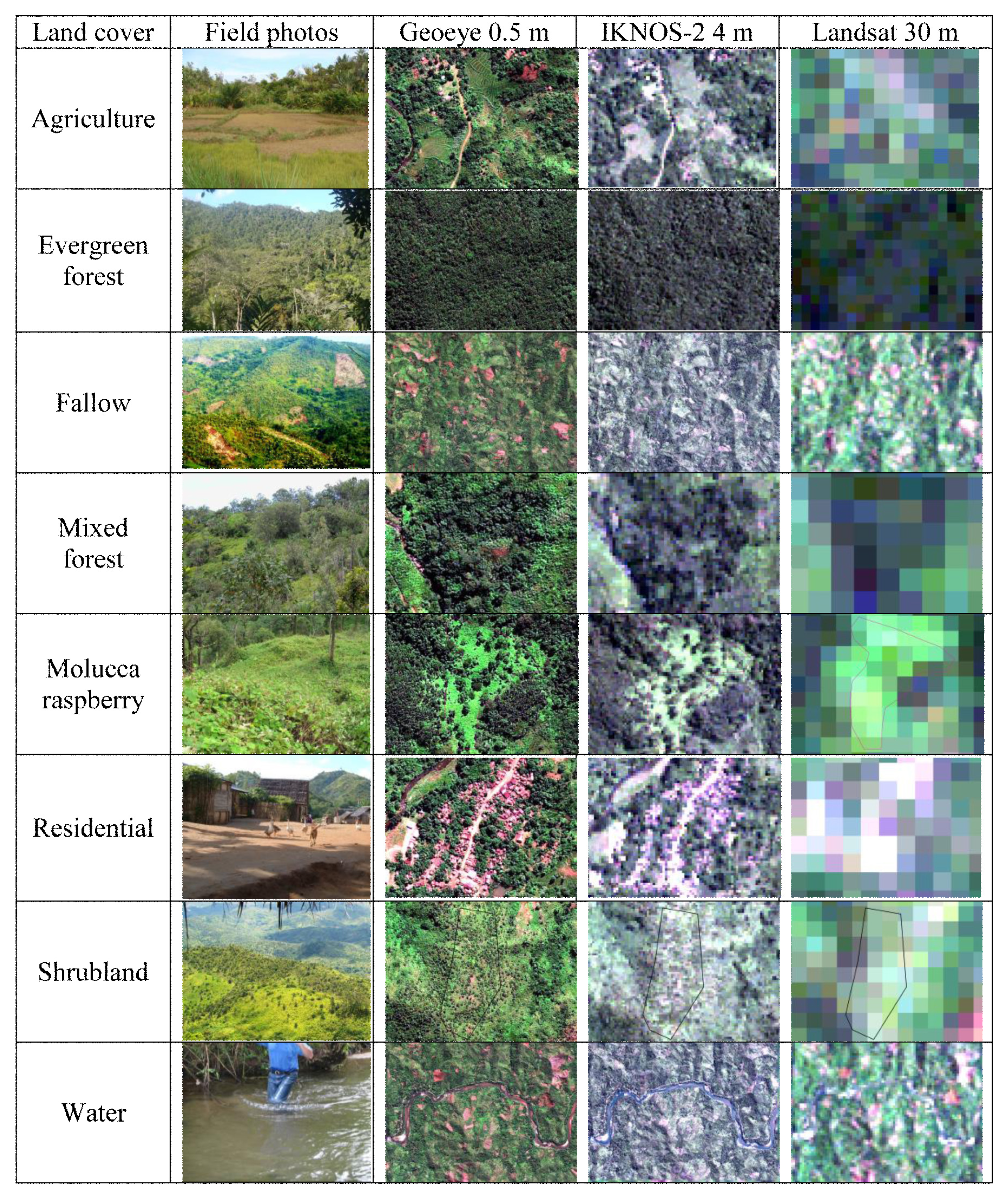
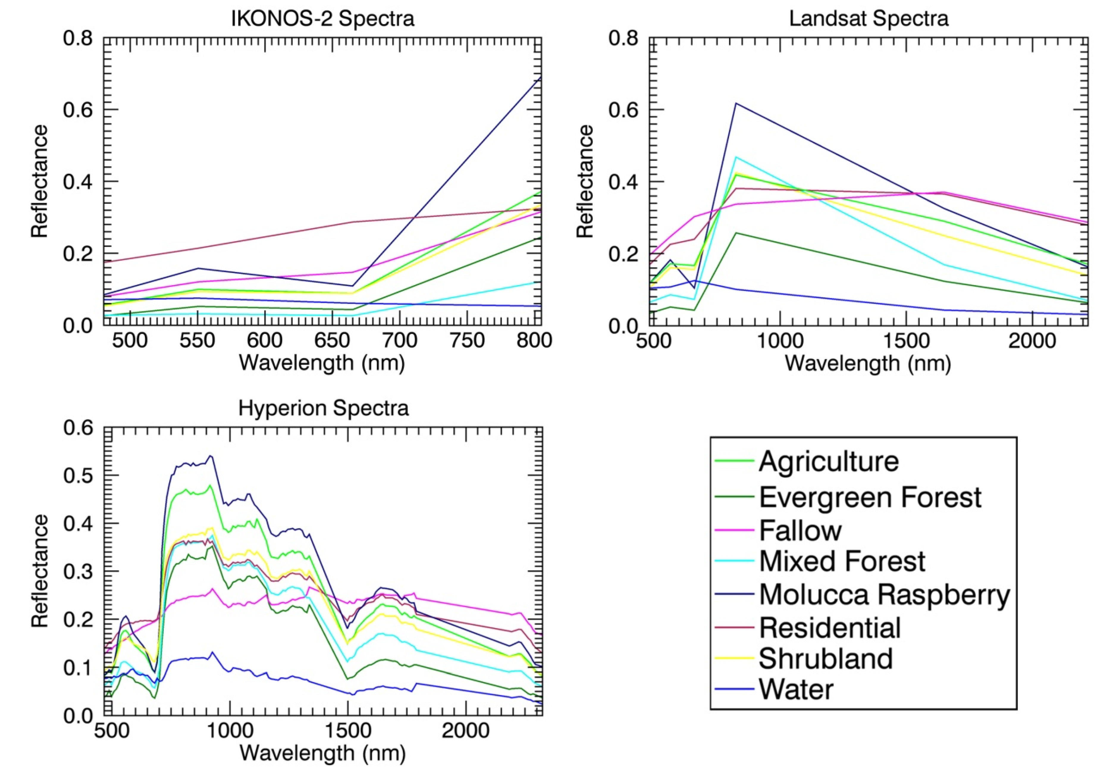
2.2. Data

| Sensor | Acquisition Date | Spatial Resolution (m) | Spectral Bands | Application |
|---|---|---|---|---|
| IKONOS | May 01, 2010 June 24, 2012 | 4 1 | 4 panchromatic | Photointerpretation for training sample selection; high resolution land cover and land use data generation; extraction of residential areas |
| Geoeye-1 Stereo | April 10, 2011 | 1.64 0.5 | 4 panchromatic | Photointerpretation for training sample selection and validation of classification results; extraction of residential areas |
| Hyperion | 10/ 27/2005 02/19/2012 | 30 | 146 117 | Invasive species detection; building spectral database |
| TM/ETM+ | 06/19/1990 04/08/1993 12/28/1996 05/16/2004 01/27/2005 04/17/2005 08/26/2006 06/10/2007 05/01/2010 02/ 21/2011 07/07/2011 | 30 | 7 | temporal dynamics of land cover and land use change |
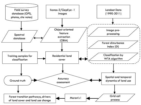
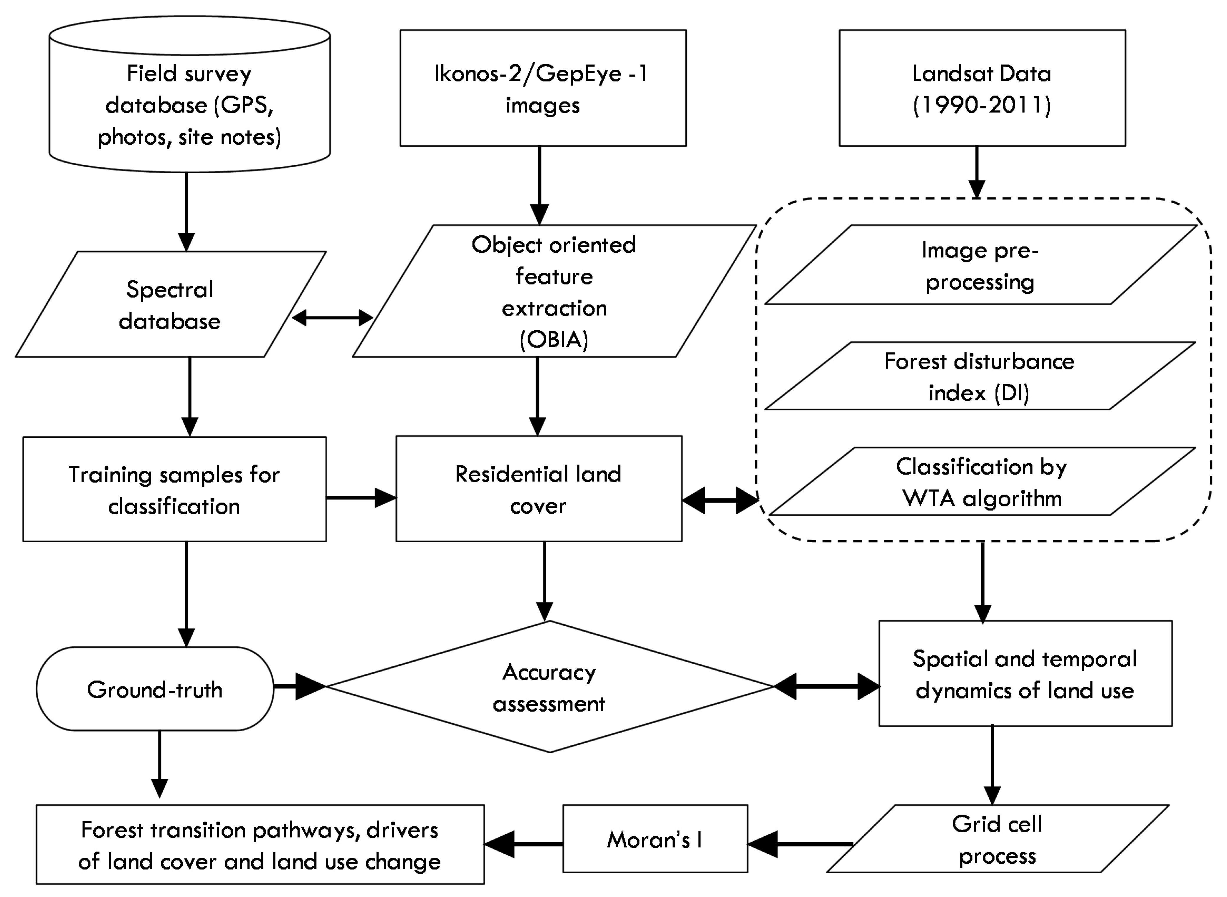
3. Methodology
3.1. Land Cover Classification


3.2. Grid Cell Processes
3.3. Moran’ I
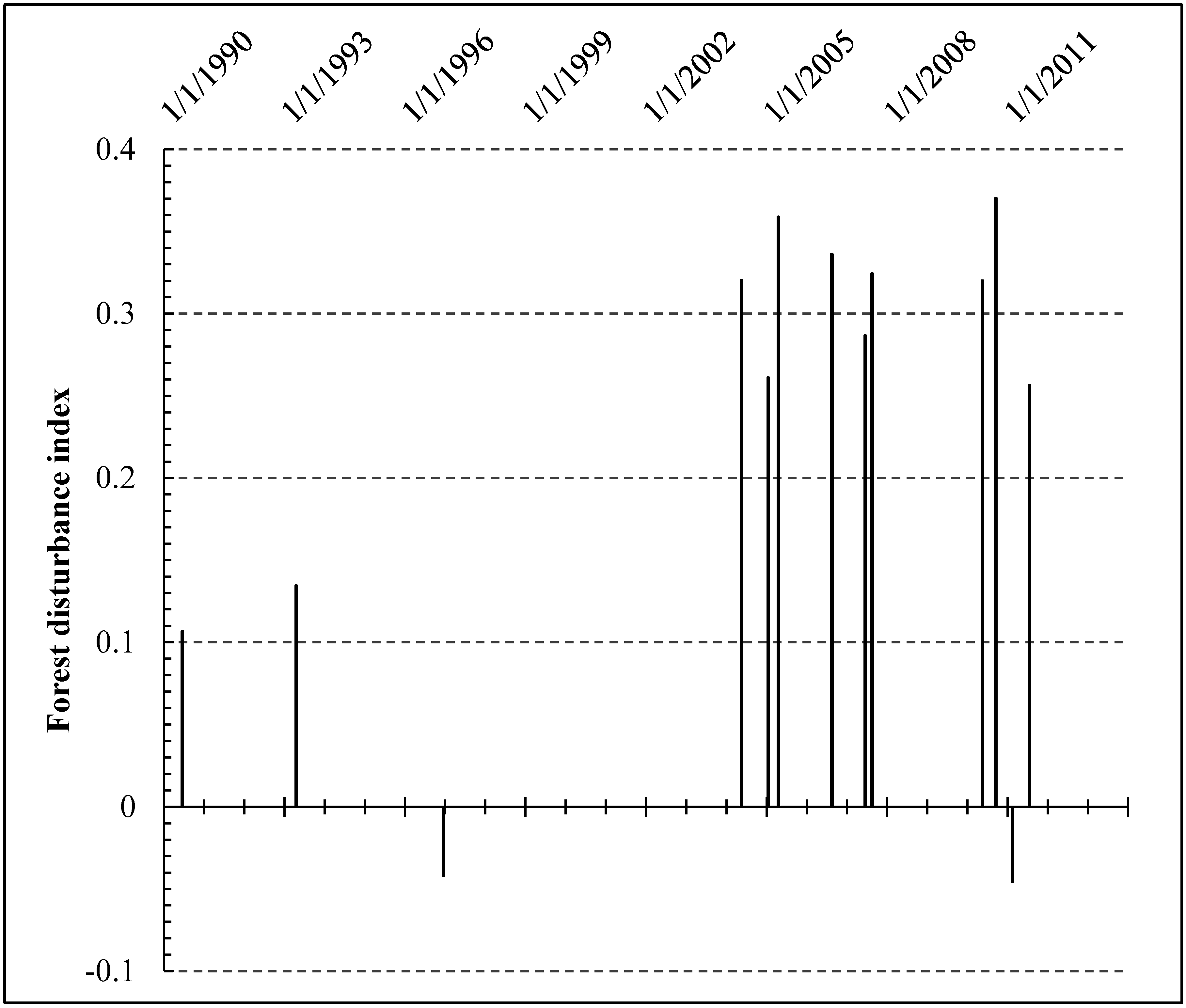
3.4. Forest Disturbance Mapping
4. Results and Discussion
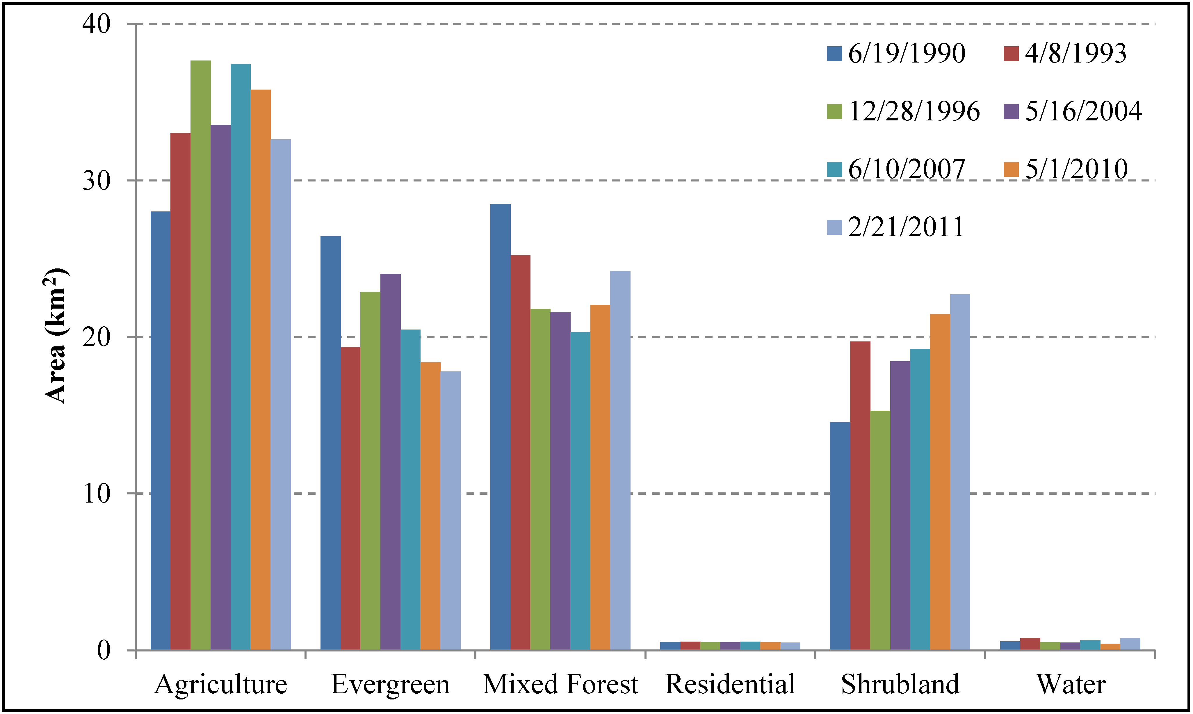
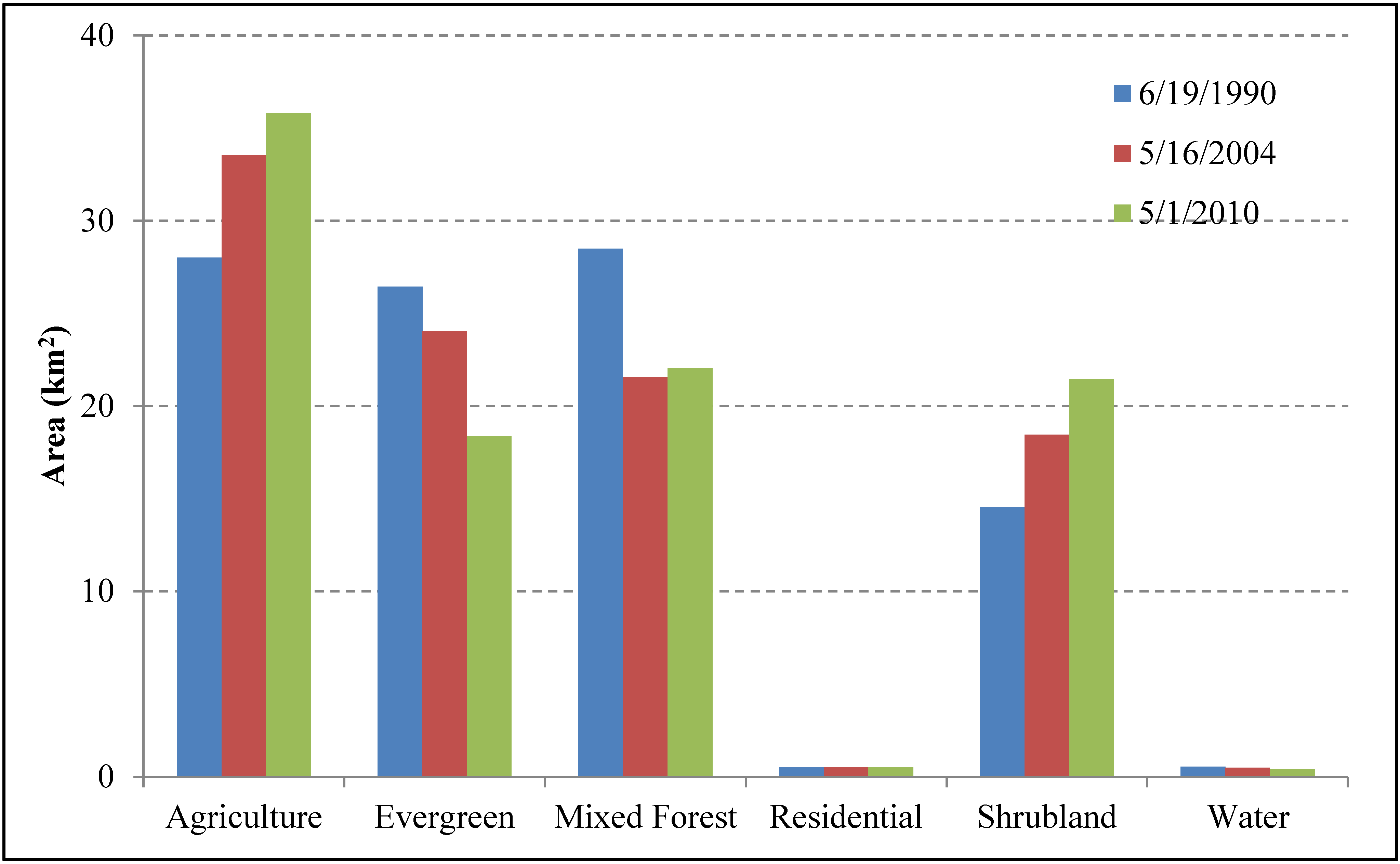
4.1. Temporal Dynamics LCLU from 1990 to 2011


| 1990 | Agriculture | Evergreen | Fallow | Mixed Forest | Shrubland | Water | Total | UA (%) |
|---|---|---|---|---|---|---|---|---|
| Agriculture | 146 | 0 | 0 | 15 | 28 | 2 | 191 | 76.44 |
| Evergreen | 13 | 315 | 0 | 21 | 6 | 0 | 355 | 88.73 |
| Fallow | 6 | 0 | 97 | 0 | 2 | 1 | 106 | 91.51 |
| Mixed Forest | 86 | 6 | 0 | 144 | 6 | 0 | 242 | 59.50 |
| Shrubland | 74 | 0 | 2 | 7 | 56 | 1 | 140 | 40.00 |
| Water | 1 | 0 | 0 | 0 | 0 | 94 | 95 | 98.95 |
| Total | 326 | 321 | 99 | 187 | 98 | 98 | 1129 | |
| PA (%) | 44.79 | 98.13 | 97.98 | 77.00 | 57.14 | 95.92 | ||
| OA (%) | 75.47 | |||||||
| Kappa | 0.71 | |||||||
| 2004 | Agriculture | Evergreen | Fallow | Mixed Forest | Shrubland | Water | Total | UA (%) |
| Agriculture | 97 | 0 | 0 | 24 | 32 | 0 | 153 | 63.4 |
| Evergreen | 1 | 315 | 0 | 25 | 2 | 0 | 343 | 91.84 |
| Fallow | 4 | 0 | 121 | 0 | 3 | 0 | 128 | 94.53 |
| Mixed Forest | 20 | 6 | 0 | 155 | 12 | 0 | 193 | 80.31 |
| Shrubland | 38 | 0 | 3 | 5 | 46 | 0 | 92 | 50.00 |
| Water | 0 | 0 | 0 | 0 | 0 | 98 | 98 | 100.00 |
| Total | 160 | 321 | 124 | 209 | 95 | 98 | 1007 | |
| PA (%) | 60.63 | 98.13 | 97.58 | 74.16 | 48.42 | 100 | ||
| OA (%) | 82.62 | |||||||
| Kappa | 0.79 | |||||||
| 2010 | Agriculture | Evergreen | Fallow | Mixed Forest | Shrubland | Water | Total | UA (%) |
| Agriculture | 158 | 0 | 0 | 11 | 0 | 0 | 169 | 81.03 |
| Evergreen | 0 | 231 | 0 | 15 | 5 | 0 | 251 | 92.03 |
| Fallow | 1 | 0 | 118 | 0 | 0 | 0 | 119 | 99.16 |
| Mixed Forest | 33 | 4 | 0 | 151 | 1 | 0 | 189 | 79.89 |
| Shrubland | 51 | 0 | 1 | 4 | 72 | 0 | 128 | 56.25 |
| Water | 0 | 0 | 0 | 0 | 0 | 98 | 98 | 100.00 |
| Total | 243 | 235 | 119 | 181 | 98 | 98 | 954 | |
| PA (%) | 65.02 | 98.3 | 99.16 | 80.75 | 73.47 | 100.00 | ||
| OA (%) | 86.79 | |||||||
| Kappa | 0.84 | |||||||
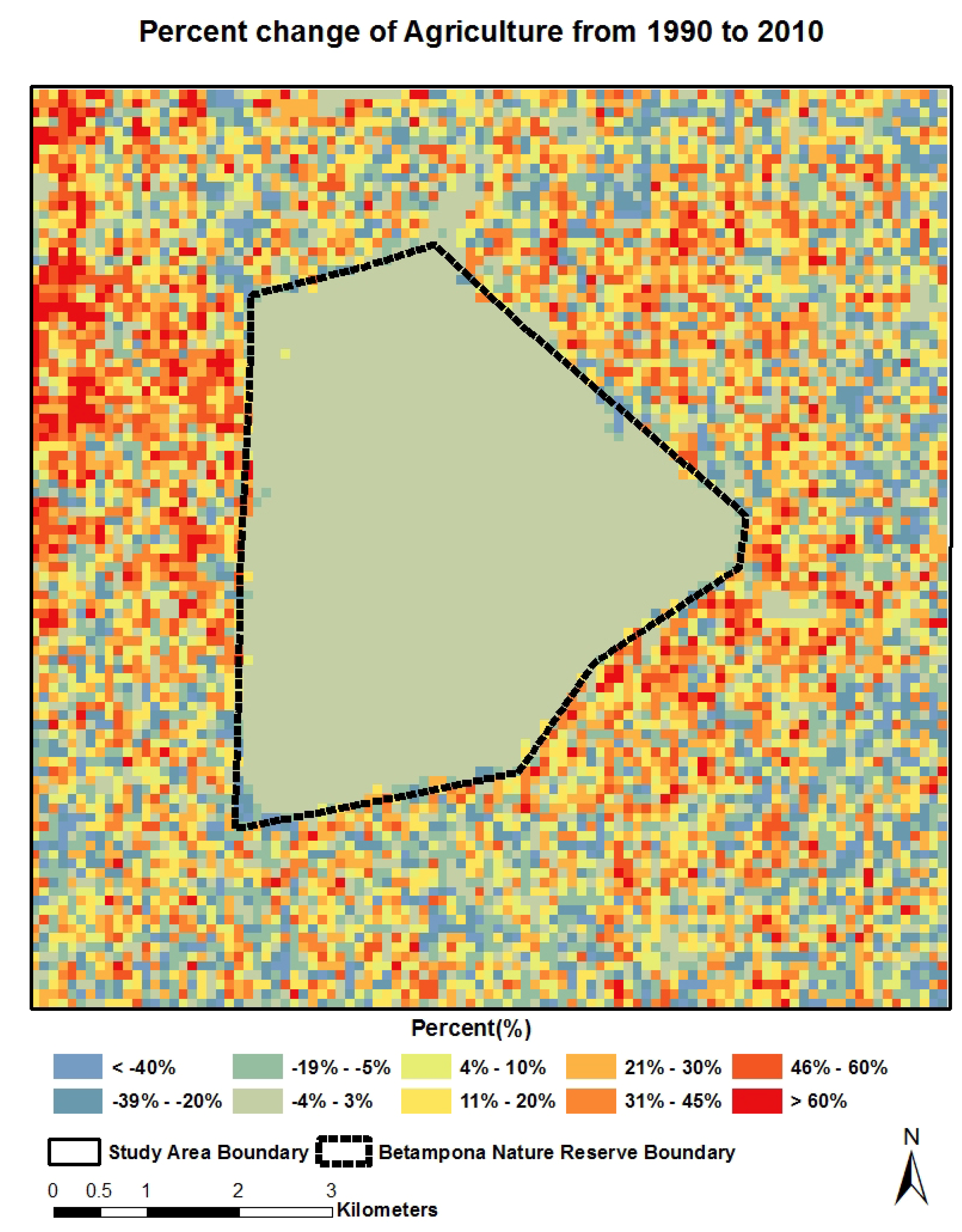
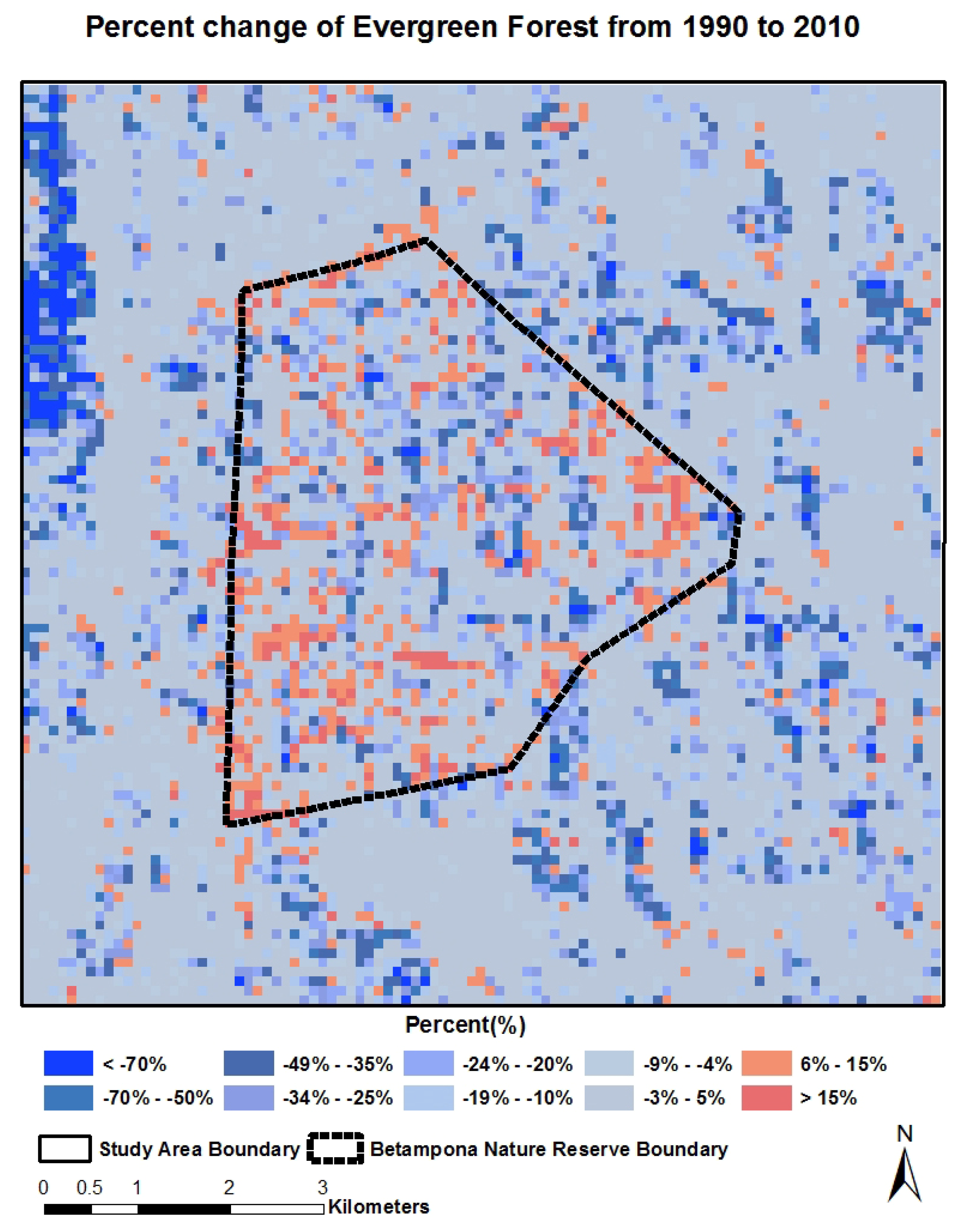
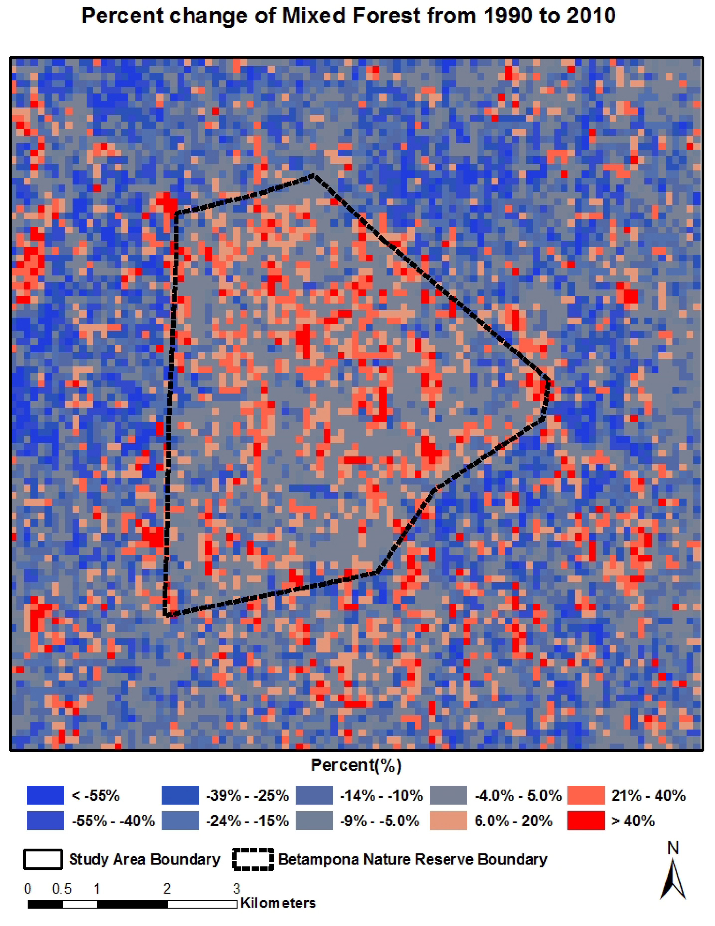
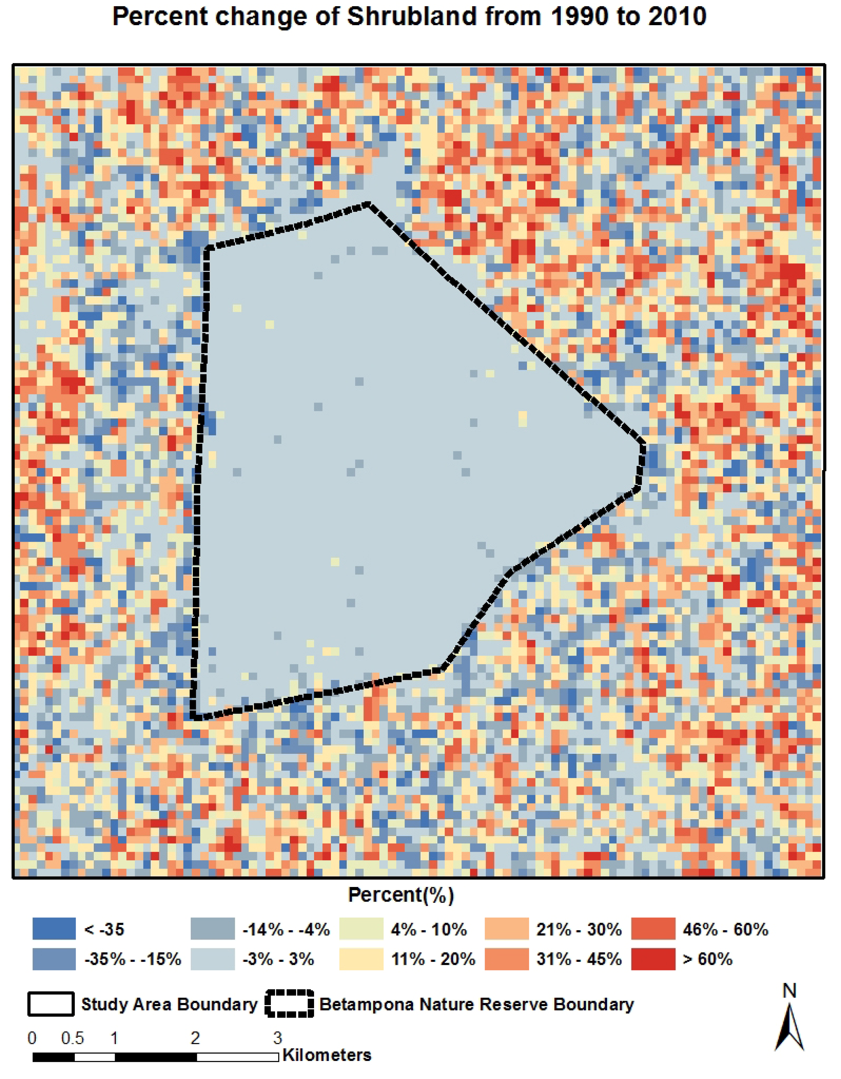
4.2. Spatial-Temporal Change of LCLU


4.3. Quantitative Relationship between Land Cover Categories

| Agriculture | Evergreen | Mixed Forest | Shrubland | |
|---|---|---|---|---|
| Agriculture | 1 | |||
| Evergreen | −0.269** | 1 | ||
| Mixed Forest | −0.465** | −0.298** | 1 | |
| Shrubland | −0.451** | −0.208** | −0.309** | 1 |

4.4. Spatial Autocorrelation Analysis for LCLU Categories
| Agriculture | Evergreen | Mixed Forest | Shrubland | |
|---|---|---|---|---|
| 1990 | 0.56 | 0.46 | 0.43 | 0.43 |
| 2010 | 0.59 | 0.55 | 0.49 | 0.55 |
4.5. Forest Disturbance

5. Conclusions
Acknowledgements
Author Contributions
Conflicts of Interest
References
- Myers, N.; Mittermeier, R.A.; Mittermeier, C.G.; da Fonseca, G.A.B.; Kent, J. Biodiversity hotspots for conservation priorities. Nature 2000, 403, 853–858. [Google Scholar] [CrossRef] [PubMed]
- Ganzhorn, J.U.; Lowry, P.P.; Schatz, G.E.; Sommer, S. The biodiversity of madagascar: One of the world’s hottest hotspots on its way out. Oryx 2001, 35, 346–348. [Google Scholar] [CrossRef]
- Dewar, R.E.; Richard, A.F. Evolution in the hypervariable environment of Madagascar. Proc. Natl. Acad. Sci. USA 2007, 104, 13723–13727. [Google Scholar] [CrossRef] [PubMed]
- Goodman, S.M.; Benstead, J.P. Updated estimates of biotic diversity and endemism for Madagascar. Oryx 2005, 39, 73–77. [Google Scholar] [CrossRef]
- Yoder, A.D.; Nowak, M.D. Has vicariance or dispersal been the predominant biogeographic force in Madagascar? Only time will tell. Annu. Rev. Ecol. Evol. Syst. 2006, 37, 405–431. [Google Scholar] [CrossRef]
- Stampoulis, D.; Haddad, Z.S.; Anagnostou, E.N. Assessing the drivers of biodiversity in Madagascar by quantifying its hydrologic properties at the watershed scale. Remote Sens. Environ. 2014, 148, 1–15. [Google Scholar] [CrossRef]
- Fifth National Report to the Convention on Biological Diversity Madagascar, Ministry of Environment and Forests, 2014; 202.
- Sala, O.E.; Chapin, F.S.; Armesto, J.J.; Berlow, E.; Bloomfield, J.; Dirzo, R.; Huber-Sanwald, E.; Huenneke, L.F.; Jackson, R.B.; Kinzig, A. Global biodiversity scenarios for the year 2100. Science 2000, 287, 1770–1774. [Google Scholar] [CrossRef] [PubMed]
- Chase, T.N.; Pielke, R.A.; Kittel, T.G.F.; Nemani, R.R.; Running, S.W. Simulated impacts of historical land cover changes on global climate in northern winter. Clim. Dynam. 2000, 16, 93–105. [Google Scholar] [CrossRef]
- Hannah, L.; Dave, R.; Lowry, P.P.; Andelman, S.; Andrianarisata, M.; Andriamaro, L.; Cameron, A.; Hijmans, R.; Kremen, C.; MacKinnon, J. Climate change adaptation for conservation in Madagascar. Biol. Lett. 2008, 4, 590–594. [Google Scholar] [CrossRef] [PubMed]
- Mace, G.M.; Norris, K.; Fitter, A.H. Biodiversity and ecosystem services: A multilayered relationship. Trends Ecol. Evol. 2012, 27, 19–26. [Google Scholar] [CrossRef] [PubMed]
- Armstrong, A.H.; Shugart, H.H.; Fatoyinbo, T.E. Characterization of community composition and forest structure in a Madagascar lowland rainforest. Trop. Conserv. Sci. 2011, 4, 428–444. [Google Scholar]
- Allnutt, T.F.; Ferrier, S.; Manion, G.; Powell, G.V.N.; Ricketts, T.H.; Fisher, B.L.; Harper, G.J.; Irwin, M.E.; Kremen, C.; Labat, J.N.; et al. A method for quantifying biodiversity loss and its application to a 50-year record of deforestation across madagascar. Conserv. Lett. 2008, 1, 173–181. [Google Scholar] [CrossRef]
- Green, G.M.; Sussman, R.W. Deforestation history of the eastern rain forests of Madagascar from satellite images. Science 1990, 248, 212–215. [Google Scholar] [CrossRef] [PubMed]
- Harper, G.J.; Steininger, M.K.; Tucker, C.J.; Juhn, D.; Hawkins, F. Fifty years of deforestation and forest fragmentation in Madagascar. Environ Conserv 2007, 34, 325–333. [Google Scholar] [CrossRef]
- Golden, C.D. Bushmeat hunting and use in the makira forest north-eastern Madagascar: A conservation and livelihoods issue. Oryx 2009, 43, 386–392. [Google Scholar] [CrossRef]
- Allnutt, T.F.; Asner, G.P.; Golden, C.D.; Powell, G.V.N. Mapping recent deforestation and forest disturbance in northeastern Madagascar. Trop. Conserv. Sci. 2013, 6, 1–15. [Google Scholar]
- Golden, C.D.; Rabehatonina, J.G.; Rakotosoa, A.; Moore, M. Socio-ecological analysis of natural resource use in Betampona strict natural reserve. Madagascar Conserv. Develop. 2014, 9, 83–89. [Google Scholar]
- Brook, B.W.; Sodhi, N.S.; Bradshaw, C.J. Synergies among extinction drivers under global change. Trends Ecol. Evol. 2008, 23, 453–460. [Google Scholar] [CrossRef] [PubMed]
- IUCN/UNEP. The LUCN Directory of Afrotropical Protected Areas; IUCN/UNEP: Gland, Switzerland and Cambridge, UK, 1987. [Google Scholar]
- Available online: http://data.worldbank.org/indicator/SP.POP.GROW/countries (accessed on 12 February 2015).
- Styger, E.; Rakotondramasy, H.M.; Pfeffer, M.J.; Fernandes, E.C.; Bates, D.M. Influence of slash-and-burn farming practices on fallow succession and land degradation in the rainforest region of Madagascar. Agric. Ecosyst. Environ. 2007, 119, 257–269. [Google Scholar] [CrossRef]
- Britt, A.; Iambana, B.; Welch, C.; Katz, A. Project Betampona: Restocking of varecia variegata variegata into the Betampona Reserve. In The Natural History of Madagascar; The University of Chicago Press: Chicago, IL, USA and London, UK, 2003; pp. 1545–1551. [Google Scholar]
- Ghulam, A.; Porton, I.; Freeman, K. Detecting subcanopy invasive plant species in tropical rainforest by integrating optical and microwave (InSAR/PolInSAR) remote sensing data, and a decision tree algorithm. ISPRS J. Photogramm. 2014, 88, 174–192. [Google Scholar] [CrossRef]
- Farris, Z.J.; Kelly, M.J.; Karpanty, S.M.; Ratelolahy, F.; Andrianjakarivelo, V.; Holmes, C. Effects of poaching, micro-habitat and landscape variables, human encroachment, and exotic species on Madagascar’s endemic and exotic carnivore community across the Masoala-Makira landscape. Biol. Conserv. Biol. 2015. submitted. [Google Scholar]
- Smith, K.; Acevedo-Whitehouse, K.; Pedersen, A. The role of infectious diseases in biological conservation. Anim. Conserv. 2009, 12, 1–12. [Google Scholar] [CrossRef]
- Deutscher, J.; Perko, R.; Gutjahr, K.; Hirschmugl, M.; Schardt, M. Mapping tropical rainforest canopy disturbances in 3D by COSMO-SkyMed spotlight InSAR-stereo data to detect areas of forest degradation. Remote Sens. 2013, 5, 648–663. [Google Scholar] [CrossRef]
- Eckert, S.; Ratsimba, H.R.; Rakotondrasoa, L.O.; Rajoelison, L.G.R.; Ehrensperger, A. Deforestation and forest degradation monitoring and assessment of biomass and carbon stock of lowland rainforest in the analanjirofo region, Madagascar. Forest Ecol. Manag. 2011, 262, 1996–2007. [Google Scholar] [CrossRef]
- Ghulam, A. Monitoring tropical forest degradation in Betampona Nature Reserve, Madagascar using multisource remote sensing data fusion. IEEE J. Sel. Top. Appl. 2014, 7, 4960–4971. [Google Scholar]
- Congalton, R.G.; Green, K. Assessing the Accuracy of Remotely Sensed Data Principles and Practices, 2nd ed.; CRC Press/Taylor & Francis: Boca Raton, FL, USA, 2009; p. 183. [Google Scholar]
- Loveland, T.R.; Merchant, J.W.; Ohlen, D.O.; Brown, J.F. Development of a land-cover characteristics database for the conterminous United-States. Photogramm. Eng. Remote Sens. 1991, 57, 1453–1463. [Google Scholar]
- Bagan, H.; Yamagata, Y. Landsat analysis of urban growth: How Tokyo became the world’s largest megacity during the last 40 years. Remote Sens Environ 2012, 127, 210–222. [Google Scholar] [CrossRef]
- Maimaitijiang, M.; Ghulam, A.; Sandoval, J.S.O.; Maimaitiyiming, M. Drivers of land cover and land use changes in St. Louis metropolitanarea over the past 40 years characterized by remote sensing andcensus population data. Int. J. Appl. Earth Obs. 2015, 35, 161–174. [Google Scholar] [CrossRef]
- Caplan, J.M.; Kennedy, L.W. Risk Terrain Modeling Manual: Theoretical Framework and Technical Steps of Spatial Risk Assessment; Rutgers Center on Public Security: Newark, NJ, USA, 2010; p. 69, (online resource). [Google Scholar]
- Moran, P.A. Notes on continuous stochastic phenomena. Biometrika 1950, 37, 17–23. [Google Scholar] [CrossRef] [PubMed]
- Healey, S.P.; Cohen, W.B.; Yang, Z.Q.; Krankina, O.N. Comparison of tasseled cap-based Landsat data structures for use in forest disturbance detection. Remote Sens. Environ. 2005, 97, 301–310. [Google Scholar] [CrossRef]
- Crist, E.P.; Kauth, R.J. The tasseled cap de-mystified. Photogramm. Eng. Remote Sens. 1986, 52, 81–86. [Google Scholar]
- Griffiths, P.; Kuemmerle, T.; Baumann, M.; Radeloff, V.C.; Abrudan, I.V.; Lieskovsky, J.; Munteanu, C.; Ostapowicz, K.; Hostert, P. Forest disturbances, forest recovery, and changes in forest types across the Carpathian ecoregion from 1985 to 2010 based on Landsat image composites. Remote Sens. Environ. 2014, 151, 72–88. [Google Scholar] [CrossRef]
- Baumann, M.; Ozdogan, M.; Wolter, P.T.; Krylov, A.; Vladimirova, N.; Radeloff, V.C. Landsat remote sensing of forest windfall disturbance. Remote Sens. Environ. 2014, 143, 171–179. [Google Scholar] [CrossRef]
- Sieber, A.; Kuemmerle, T.; Prishchepov, A.V.; Wendland, K.J.; Baumann, M.; Radeloff, V.C.; Baskin, L.M.; Hostert, P. Landsat-based mapping of post-Soviet land-use change to assess the effectiveness of the Oksky and Mordovsky protected areas in European Russia. Remote Sens. Environ. 2013, 133, 38–51. [Google Scholar] [CrossRef]
- Braat, L.; ten Brink, P.; Eds.; with Bakkes, J.; Bolt, K.; Braeuer, I.; ten Brink, B.; Chiabai, A.; Ding, H.; Gerdes, H.; Jeuken, M.; Kettunen, M.; Kirchholtes, U.; Klok, C.; Markandya, A.; Nunes, P.; van Oorschot, M.; Peralta-Bezerra, N.; Rayment, M.; Travisi, C.; Walpole, M. The Cost of Policy Inaction (COPI): The Case of not Meeting the 2010 Biodiversity Target; European Commission: Brussels, 2008; p. 58. [Google Scholar]
- Kumar, P. (Ed.) The Economics of Ecosystems and Biodiversity Ecological and Economic Foundations; Kumar, P. (Ed.) Earthscan: London, UK and Washington, DC, USA, 2010; Figure 6 (See p. 18).
- Lockwood, J.; Hoopes, M.; Marchetti, M. Invasive Ecology; Blackwell Publ.Ltd.: Oxford, UK, 2007; p. 304. [Google Scholar]
© 2015 by the authors; licensee MDPI, Basel, Switzerland. This article is an open access article distributed under the terms and conditions of the Creative Commons Attribution license (http://creativecommons.org/licenses/by/4.0/).
Share and Cite
Ghulam, A.; Ghulam, O.; Maimaitijiang, M.; Freeman, K.; Porton, I.; Maimaitiyiming, M. Remote Sensing Based Spatial Statistics to Document Tropical Rainforest Transition Pathways. Remote Sens. 2015, 7, 6257-6279. https://0-doi-org.brum.beds.ac.uk/10.3390/rs70506257
Ghulam A, Ghulam O, Maimaitijiang M, Freeman K, Porton I, Maimaitiyiming M. Remote Sensing Based Spatial Statistics to Document Tropical Rainforest Transition Pathways. Remote Sensing. 2015; 7(5):6257-6279. https://0-doi-org.brum.beds.ac.uk/10.3390/rs70506257
Chicago/Turabian StyleGhulam, Abduwasit, Oghlan Ghulam, Maitiniyazi Maimaitijiang, Karen Freeman, Ingrid Porton, and Matthew Maimaitiyiming. 2015. "Remote Sensing Based Spatial Statistics to Document Tropical Rainforest Transition Pathways" Remote Sensing 7, no. 5: 6257-6279. https://0-doi-org.brum.beds.ac.uk/10.3390/rs70506257