Empirical Radiometric Normalization of Road Points from Terrestrial Mobile Lidar System

Abstract

Lidar data provide both geometric and radiometric information. Radiometric information is influenced by sensor and target factors and should be calibrated to obtain consistent energy responses. The radiometric correction of airborne lidar system (ALS) converts the amplitude into a backscatter cross-section with physical meaning value by applying a model-driven approach. The radiometric correction of terrestrial mobile lidar system (MLS) is a challenging task because it does not completely follow the inverse square range function at near-range. This study proposed a radiometric normalization workflow for MLS using a data-driven approach. The scope of this study is to normalize amplitude of road points for road surface classification, assuming that road points from different scanners or strips should have similar responses in overlapped areas. The normalization parameters for range effect were obtained from crossroads. The experiment showed that the amplitude difference between scanners and strips decreased after radiometric normalization and improved the accuracy of road surface classification.

1. Introduction

Light detection and ranging (lidar) is an active remote sensing system that can effectively acquire the 3D spatial coordinates of the target. The lidar system provides both geometric and radiometric information to identify different objects. The lidar radiometric information can be applied in visualization, segmentation, and classification of point clouds but is influenced by the material of target, system factors, geometric factors between the target and sensor (i.e., distance and incident angle), and atmospheric conditions [1,2]. Hence, lidar should be calibrated to obtain uniform radiometric information for further applications.

The lidar intensity measurement can be converted into radiometric quantities with physical properties like backscattering coefficients. The radiometric correction of lidar system can be classified into two categories: model-driven and data-driven approaches [3]. The model-driven approach uses a physical mathematic model from the lidar equation [4,5,6,7,8] to convert lidar amplitude to a backscattering cross-section or backscattering coefficient [9,10] with physical meaning. The model-driven approach has been widely applied to airborne lidar system (ALS) radiometric correction in different models. This approach calculates the calibrated constant (Ccal), a constant with physical meaning derived from the lidar equation, based on the reflectance of reference targets. The calibrated constant is then applied to all lidar points to obtain the backscattering cross-sections. In contrast, the data-driven approach uses an empirical mathematic model derived from the dataset itself. The empirical function can be a function of range, incident angle or automatic gain control (AGC) [3,11,12,13,14,15]. This approach selects several homogeneous regions as control patches in overlapping areas. The control patches are used to calculate the correction parameters of the empirical model by least squares adjustment. The correction parameters are then applied to normalize the radiometrical difference between points.

Lidar systems are available on several different platforms, such as ALS and terrestrial lidar systems (TLS). Several studies have developed radiometric correction methods for ALS. With the development of full-waveform lidar, Wagner et al. (2006) [16] used the range, pulse width, amplitude, and incident angle to calibrate small-footprint, full-waveform ALS. Höfle and Pfeifer (2007) [3] compared calibration results with model-driven and data-driven approaches at different heights and different trajectories using “range” only to form different empirical calibration functions, while Jutzi and Gross (2009) [11] considered both “range” and “surface incidence angle” to form an empirical calibration function. In addition, Ding et al. (2013) [12] considered both diffuse and specular reflectance with the Phong model for wet- or water-dominated areas.

The fundamental equation in ALS radiometric correction inverses the received power to square range; however, the 1/r² correction cannot be directly applied to TLS. Due to internal system factors such as brightness reducer, AGC [17], or receiver optics [18,19], the radiometric correction of TLS is more complex than ALS and does not completely follow the inverse square range function (1/r²) [20,21,22,23]. Because the TLS data, particularly TLS intensity at near range, cannot simply use the lidar equation in model-driven approach, most TLS radiometric processing uses the data-driven approach [17,20,21,22,23,24,25].

To understand the range effect on TLS intensity, Pfeifer et al. (2008) [20] used Riegl LMS-Z420i and Optech ILRIS-3D to measure different Spectralon targets at different distances. The observations were applied to from mathematic functions between observed intensity from the range and reflectivity of the targets. Because of the effect of near-distance brightness reducer, the behavior of near range was different from reflectivity. Therefore, a separation approach was applied to split the functions into two correction functions based on range. Kaasalainen et al. (2009) [17] also indicated the effect of near-distance brightness reducer for FARO LS HE80 from laboratory measurement and applied a logarithmic correction function for radiometric correction. Kaasalainen et al. (2011) [22] further investigated the incident angle and range effects on TLS using reference targets. The experimental results indicated that the range effect is mainly dominated by instrumental factors, and that the lidar equation correction can only be used after 10–15 m distance. The angle effect, however, is mainly related to target surface properties, and the behavior was similar to Lambertian (cosine) scattering law. The reflectance is related to material, physical properties (e.g., albedo, grain size), conditions (e.g., dry, wet) and others. In the radiometric correction for lidar system, the previous studies selected the asphalt road surface as a reference target to calculate the calibration coefficient of a lidar equation. As the road surface is a homogeneous reflecting surface and it behaves like Lambertian scatterer [5,16] than other material, so asphalt roads have been used for deriving the calibration constant based on an assumed value or field-measured reflectance value.

There are a number of applications for radiometric corrected lidar data. Radiometric correction not only improves the radiometric consistence between lidar systems, it also provides physical radiometric quantities (e.g., backscattering) to separate different objects [2]. Moreover, it is also beneficial for point cloud segmentation [15]. Radiometric correction is an important process in the integration of multi-station (or multi-strip) lidar systems. For example, Höfle (2014) [26] performed radiometric correction for multi-station TLSs in maize plant detection. Radiometric correction is especially important in the development of multispectral lidar to integrate received power from different wavelengths [27]. For example, Hartzell et al. (2014) [28] developed multispectral TLS by integrating three different wavelength lidar systems and implemented the radiometric calibration of the different lidar systems to classify different rock types. Fang et al. (2015) [19] developed a near-distance intensity correction for TLS data that significantly improved the digital preservation of wall-painting in World Heritage Sites.

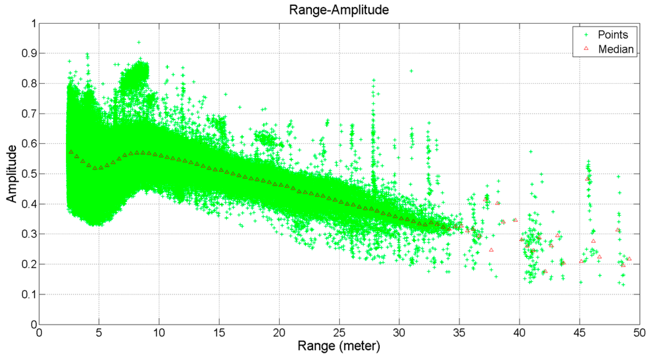
Terrestrial mobile lidar system (MLS) usually contains multiple laser scanners to obtain a complete scene of road environments from different scanning directions. For example, Riegl VMX250 and Optech Lynx M1 have two laser units that scan in perpendicular directions. Another method to obtain a more complete scene of road environments is obtaining data from multiple strips, such as forward and reversed trajectories. As the road points from MLS are scanned from different laser units or different trajectories, the intensity of road points should be corrected or normalized to have uniform value. Most previous studies focused on radiometric correction for ALS and TLS; the radiometric processing for MLS is still sparsely available. The challenge of MLS radiometric correction is that the lidar equation for ALS cannot be directly applied to MLS. It does not completely follow the inverse square range function (1/r²) (Figure 1). In addition, the MLS obtains 3-D points in a dynamic platform and is more complicated than static TLS.

Figure 1. An example of range-amplitude for MLS: the behavior of near-range is different from theoretical lidar equation.

Figure 1. An example of range-amplitude for MLS: the behavior of near-range is different from theoretical lidar equation.

The aim of this research was to establish an empirical radiometric normalization for MLS road points. We assumed that conjugate asphalt roads from different laser scanners or strips would respond similarly, and range effect was considered in radiometric normalizations. The proposed scheme was a data-driven approach, and this empirical model was obtained from crossroads. The scope of this study was to normalize road points for road surface classification, and therefore, non-road points such as vehicles and buildings were removed in this study. The contributions of this study were (1) to establish an empirical radiometric normalization processing for MLS; and (2) to compare the original and normalized points in road surface classification. The major work established and applied normalization models for road surface classification. In addition, the validation of proposed method included (1) the consistency of lidar amplitude before and after normalization; and (2) the accuracy of road surface classification.

2. Study Area and Dataset

This study used mobile lidar data acquired by Riegl VMX-250 [29], which consists of two Riegl VQ-250 laser scanners, four 5MP digital cameras, and a positioning and orientation system (POS). The minimum and maximum laser range measurements were 1.5 m and 500 m. Because the scanning mechanism of VQ-250 laser scanner belongs to a rotating polygon, the laser scanner has a 360°, full circle field-of-view in a near vertical direction. Its ground patterns are parallel scan lines. The laser beam shoots on the continuous rotation polygon mirror surface and is then reflected to the ground to form a continuous strip and parallel scan lines. The intersection angle of these two scanners is about 135° to avoid the object’s occlusion.

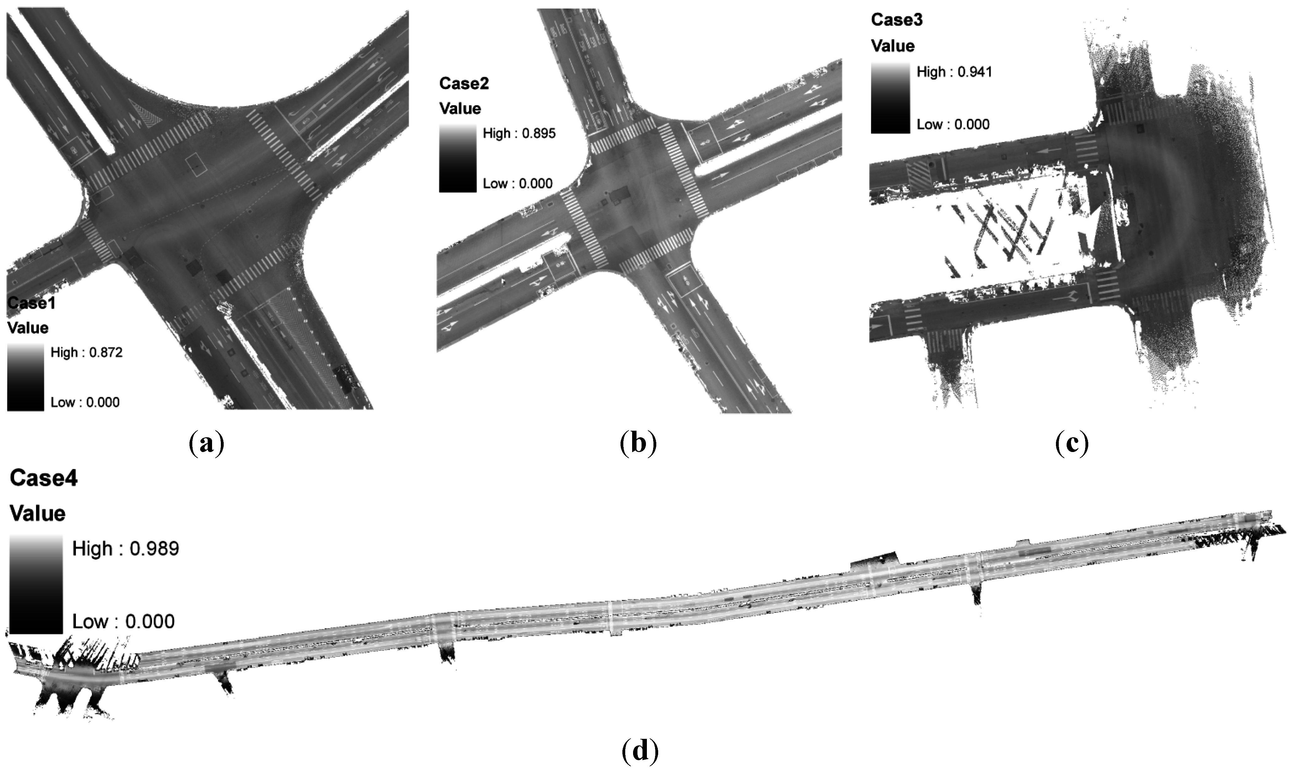
The test area was located at Taipei City, and four datasets (Figure 2) with different characteristic were selected to evaluate the proposed method. The road surface is ordinary, new asphalt pavement with colored road markings (e.g., white, yellow, and red). Case 1 is a crossroad consisting of four strips. Because this area contains the least non-road object interference, it was selected as a reference to establish an empirical normalization model and calculate radiometric normalization coefficients. Once the radiometric normalization coefficients were determined, these coefficients were applied to all other cases from same system. Case 2 is another crossroads with four strips. Case 3 is a U-turn lane with one continued strip. It was included to illustrate that radiometric normalization is necessary even with a single strip. Case 4 is a linear road with two opposite strips. This road type is the most common in MLS and was used here to demonstrate the radiometric normalization with a wider area. Table 1 summarizes the information of four datasets.

Table 1. Summary of test area.

	Case 1 (Reference Area)	Case 2	Case 3	Case 4
Road type	Crossroads	Crossroads	U-turn lane	Linear road
Number of Strips	4	4	1	2
Size	100 m × 100 m	100 m × 100 m	100 m × 100 m	1400 m × 50 m

Table 1. Summary of test area.

	Case 1 (Reference Area)	Case 2	Case 3	Case 4
Road type	Crossroads	Crossroads	U-turn lane	Linear road
Number of Strips	4	4	1	2
Size	100 m × 100 m	100 m × 100 m	100 m × 100 m	1400 m × 50 m

Figure 2. Test data colored by normalized amplitude: (a) case 1, (b) case 2, (c) case 3, and (d) case 4.

Figure 2. Test data colored by normalized amplitude: (a) case 1, (b) case 2, (c) case 3, and (d) case 4.

3. Proposed Scheme

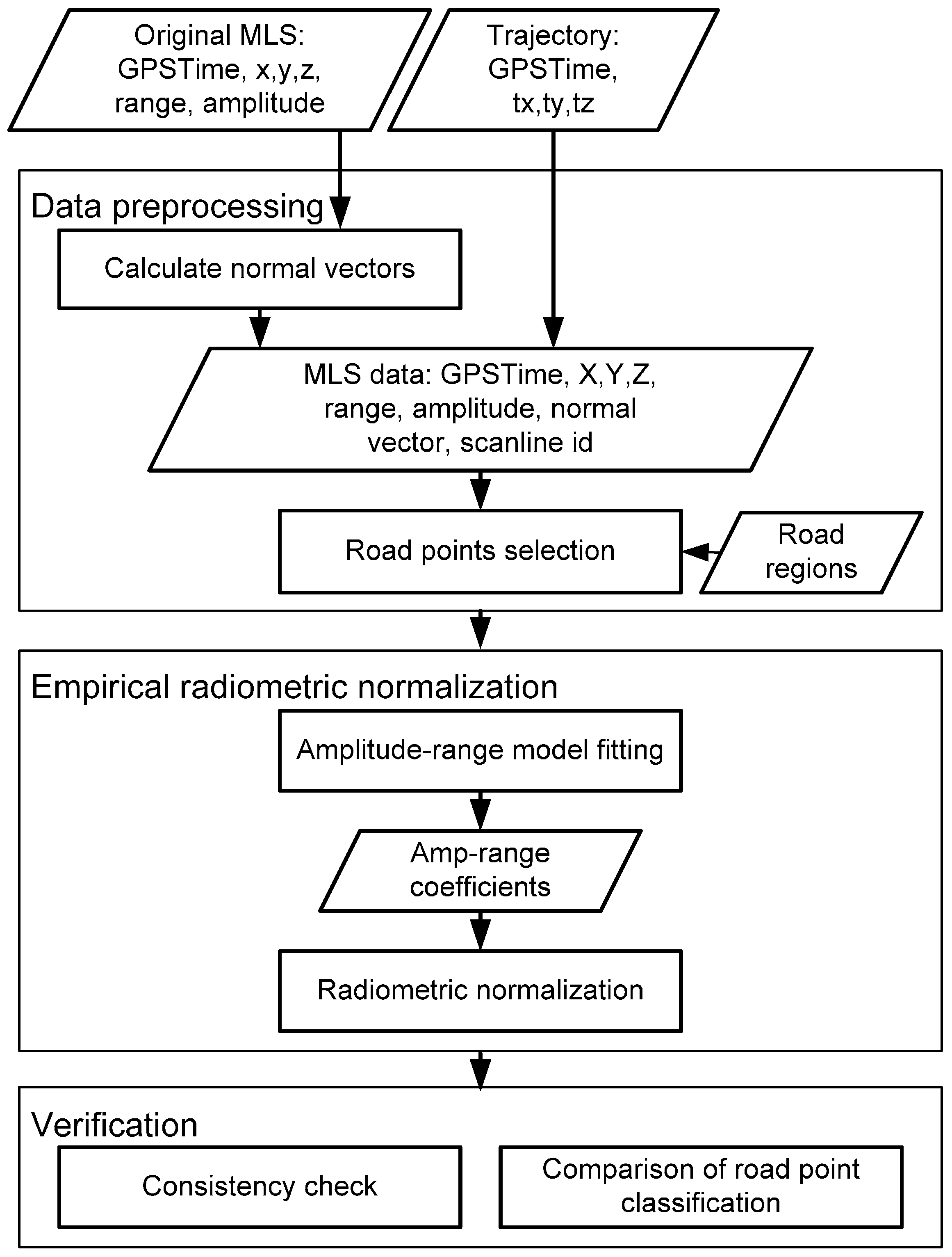
The framework (Figure 3) consisted of three major parts: (1) data preprocessing; (2) empirical radiometric normalization; and (3) evaluation using consistency check and road surface classification. In Section 3.1, we calculated the normal vector of the lidar point and extracted the road point. Because our focus is road points, we removed the non-road points using normal vector and estimated road surface height and additional road region polygons from the vector map. In Section 3.2, range was the major factor in radiometric normalization, so we used different empirical models to find the relationship between range and amplitude. Finally, the proposed models were evaluated by consistency checks and road surface classification in Section 3.3.

3.1. Data Pre-Processing

The input data included (1) original MLS data, (2) adjusted trajectory data from the POS, and (3) the 2-D road region from the vector map. Each lidar point in the original MLS data contain GPS time, X, Y, Z, range between laser center and object, and amplitude of echo. Because our focus was road points, the role of the 2-D road region from vector map was to exclude the non-road region.

Figure 3. The framework of MLS radiometric normalization.

Figure 3. The framework of MLS radiometric normalization.

Figure 4. Extraction of scan line (colored by scan line ID).

Figure 4. Extraction of scan line (colored by scan line ID).

The data pre-processing included three major works: (1) indexing the scan line, (2) calculating the surface normal vector from lidar points, and (3) road point selection. Separating different scan lines is a core process in radiometric normalization and is used to determine the relationship of amplitude and range in one scan line. In this study, the scanning mechanism of test data was a 360°, full circle rotating mirror. The duration time of a scan line is fixed by predefined scanning rates (i.e., 0.01 sec/scan in our study). Assuming that the GPS time for the first point of a project is t₀ and the duration time of a scan line is dt, the points within t₀ to t₀ + dt are classified onto a scan line. As the test area in this study is relatively simple than other cases, the results of the previous method and this refined method are the same. The scan line identification can be used to calculate the length of range for a scan line. So, we select the longest scan line to observe the relationship between amplitude and range. Besides, the sequential points on a scan line can be used to determine the height jump between points. It can be used to remove the non-road points. In scan line extraction, different colors indicate different scan lines (Figure 4), illustrating that the scan lines are distributed along the MLS trajectory.

The normal vector of a lidar point can be used in road point selection. The normal vector is obtained by plane fitting of the nearest lidar points within a certain distance. In this study, the search radius was 0.5 m, and the lidar points within this radius were selected for plane fitting. The plane equation shown in equation 1 is representative of a plane in any direction. After the plane fitting, the normal vector is calculated from plane coefficients, as shown in Equation (2). For complex targets like façades from MMS, the sequential points should be considered and the original points can be converted to sensor-oriented coordinate system to maximize the consistency within points [30]. For complex targets from ALS, the point selection plays an important role in normal vector calculation. Abed et al. (2012) [31] proposed a Robust Surface Normal (RSN) estimation method based on the K-nearest neighbors selection algorithm. On the other hand, Lin et al. (2014) [32] used the weighted covariance matrices to refine the normal vector in ALS. In this study, the simple plane fitting is applied to road surface as it is homogenous and relatively simple than other complex objects.

$$Ax+By+Cz=D$$

(1)

$$n_x=A;n_y=B;n_z=C$$

(2)

where

• x, y, z = coordinates of lidar point;
• A, B, C, D =coefficients of a plane; and
• n_x, n_y, n_z = normal vector of a plane.

The last step of data pre-processing is non-road point removal. Our normalization target was based on asphalt road, but objects such as pedestrians, vehicles, traffic signals, and trees will influence the result. There are three major steps to non-road point removal. (1) Road region from vector map: the road polygons from the vector map define the boundaries of road, and we exclude the lidar points outside of the defined road region. (2) Normal vector criteria: if the normal vector of a lidar point is not in a near-vertical direction, this lidar point might not locate on road surface; therefore, if the angle between the normal vector and the Z-axis is greater than 5°, this lidar point was treated as a non-road point. This step can determine if the point is located on the plane, but some points above the road surface (e.g., top of the car) cannot be removed and elevation threshold is required. (3) Elevation threshold: to remove a flat point above the road surface, we used the heights of the trajectory and the vehicle to estimate the elevation of road surface. The non-road points can be removed if the elevation of the lidar points exceeds the estimated elevation.

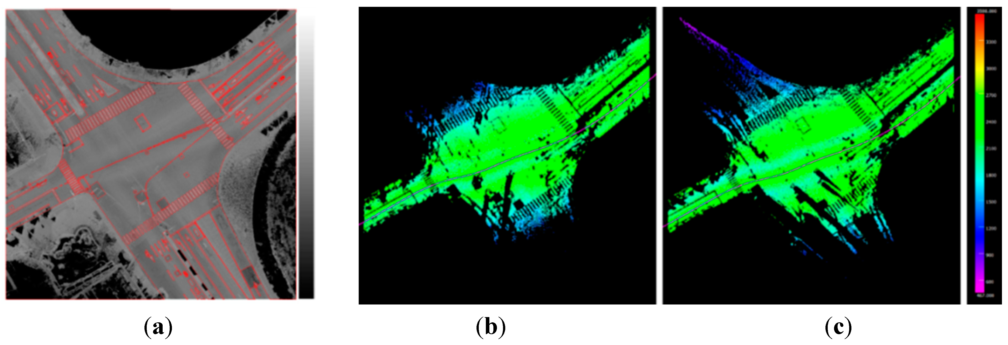
After data preprocessing, the selected lidar points contain asphalt road and road markings. Because case 1 was selected as a reference area to establish empirical normalization model, the white-colored road marks and black-colored new pavement may affect the model fitting; therefore, additional processing is needed to remove the road mark. We digitized the road marks and new pavements and produced a mask to remove these non-asphalt road regions (Figure 5a–c).

Figure 5. Extraction of road points for case 1: (a) additional manual digitization of road marks, (b) scanner 1 (colored by amplitude), and (c) scanner 2 (colored by amplitude).

Figure 5. Extraction of road points for case 1: (a) additional manual digitization of road marks, (b) scanner 1 (colored by amplitude), and (c) scanner 2 (colored by amplitude).

3.2. Empirical Radiometric Normalization

We used the amplitude-range function to remove the distance effect for the recorded amplitude. Due to the near distance effect on TLS, the recorded amplitude behavior deviates from an ideal physical lidar equation at near distance [19,20,22]. In other words, the recorded amplitude of TLS is not entirely proportional to 1/r² in the lidar equation. The data-driven approach is usually applied to the radiometric correction of TLS. There are two possibilities to collect the reference dataset for data-driven approach. One is to collect the amplitudes from signalized Spectralon targets at different ranges [26] and then apply the collected amplitudes and ranges to estimate the amplitude-range function. An alternate method is to measure the amplitude from available natural field targets. For example, asphalt roads exhibit stability for the radiometric correction of ALS [2]. Most of the TLS used the signalized Spectralon targets at different ranges for radiometric correction. The position of TLS and target are fixed in data collection. For MLS, the laser scanning mechanism is a line scanner mounted on a moving platform. As for the dynamic lidar sampling and moving platform, the natural field target like asphalt road is more favorable for radiometric correction of MLS. We assume that the asphalt road at different ranges should have similar amplitude after radiometric normalization; therefore, this study used asphalt road as a reference target to determine the amplitude-range function.

Because most manufacturers do not provide detailed system parameters to implement the model-driven approach, empirical functions were adopted in this study. Several studies indicated that the intensity of TLS was proportional to 1/r² after 10 m to 15 m distance [21,22], which means that the near range and non-near range are two different functions. In this study, a separation approach [20] was applied to estimate the amplitude-range functions, using two low-order polynomial functions rather than a high-order polynomial function. The advantage of separation approach is to avoid over-fitting in high-order polynomial functions.

The scan lines from case 1 were selected as a reference dataset to determine the amplitude-range function. The non-asphalt road points in case 1 were removed in a previous step, and therefore only the asphalt road points were utilized to estimate the amplitude-range function. The proposed separation approach included two major steps: (1) separation point determination; and (2) polynomial functions fitting.

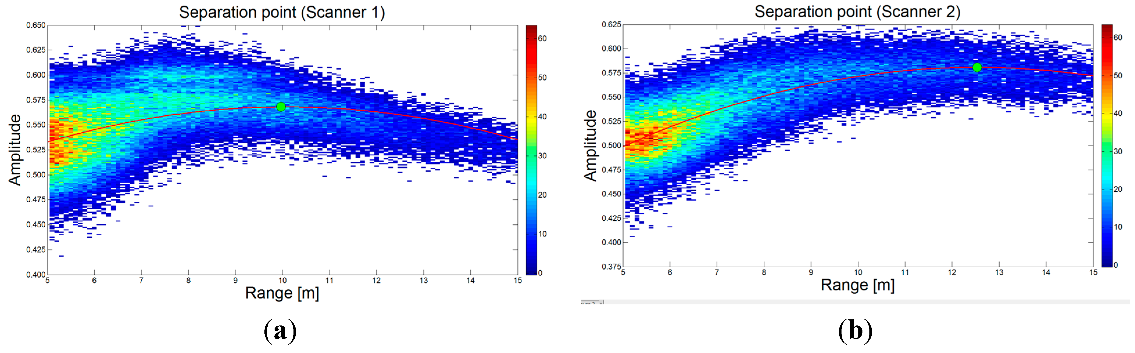
To separate the amplitude-range function into two functions, we determined a separation point for near-range and far-range. Previous studies found that the turning point is around 10 m; hence, we selected the lidar points within 5 m to 15 m distances to determine the separation point. All the selected lidar points were applied in a second-order amplitude-range polynomial fitting. The peak of this function was then treated as a turning point to distinguish near-range and far-range points. In this study, the separation point refers to the turning point of the second-order polynomial function. In the separation point estimation for scanners 1 and 2 in case 1 (Figure 6), the red line is a second-order polynomial function while the circle is the estimated separation (turning) point. The calculated separation points for scanners 1 and 2 were 9.98 m and 12.54 m, respectively. The difference between scanner 1 and scanner 2 is about 2.5 m. The sources of discrepancy in separation range between these two laser scanners might be: the system parameters for two logarithmic amplifiers are not the same; or, the near distance reducers might use different system parameters in these two laser units.

Figure 6. Extraction of separation points: (a) scanner 1 (colored by number-of-point in a cell) and (b) scanner 2 (colored by number-of-point in a cell).

Figure 6. Extraction of separation points: (a) scanner 1 (colored by number-of-point in a cell) and (b) scanner 2 (colored by number-of-point in a cell).

Once the separation point was determined, two polynomial functions were chosen to model the relationship between amplitude and range. We used a function of range, as shown in Equation (3), for near-range data. A polynomial function based on range was adopted in the modeling of amplitude-range behavior. The trend of amplitudes in far range was decreasing while the range was increasing. As the amplitude of MLS was proportional to 1/r after the separation point, we used a function of inverse-range (i.e., 1/r, Equation (3)) to model the amplitude-range relation. A least squares fitting technique was applied to optimize the polynomial coefficients. We have removed most of the outliers in the stage of data preprocessing (Section 3.1) as the least square method is not robust against the outliers. A huge amount of lidar points need excessive computational resources. In order to reduce the points and also improve the computational efficiency, we use range-amplitude distribution (i.e., x-axis is range and y-axis is amplitude) to remove the inconsistent points. We calculate the moving mean and the standard deviation along the range direction. Then, we select the points within ± 1 sigma for least squares fitting. Therefore, the majority points for least squares fitting are asphalt road points. After point reduction, the number of road points for scanners 1 and 2 are 1,162,391 and 1,134,137 points. To avoid discontinuities at separation point (r_sp), the positional continuous functions (C° continuous) and first-order differential equations (C¹ continuous) were added to constrain the continuity (see Equations (4) and (5)). Finally, f(r) was used as a normalized factor to convert the original recorded amplitude into normalized amplitude (Equation (6)). Because the fitting result will influence the normalization process, the optimal polynomial order is needed. The lowest root mean square error (RMSE) was chosen to be a standard function and was applied to the normalization process.

$$f(r)=\{\begin{array}{c}{f}_1(r)=a_0+a_{1}r+a_2{r}^2+\mathrm{...}+a_n{r}^n,r\le r_{sp}\\ f_2(r)=b_0+b_1\frac{1}{r}+b_2\frac{1}{r^2}\begin{array}{cc}+\mathrm{...}& +b_n\frac{1}{r^n}\end{array},r>r_{sp}\end{array}$$

(3)

$$f_1\left(r_{sp}\right)=f_2\left(r_{sp}\right)$$

(4)

$$f_1^{\text{'}}\left(r_{sp}\right)=f_2^{\text{'}}\left(r_{sp}\right)$$

(5)

$$A_n=\frac{A_o}{f\left(r\right)}$$

(6)

where

• f₁(r) = polynomial function for near-range;
• f₂(r) = polynomial function after separation point;
• r = range;
• r_sp = range at separation point;
• a₀~a_n, b₀~b_n = polynomial coefficients to describe the range effect;
• A_o = original amplitude; and
• A_n = normalized amplitude.

3.3. Verification

3.3.1. Consistency Check

Because our aim was to reduce the radiometric difference between different strips or scanners in overlapped regions in which the amplitudes from different strips or scanners should have similar responses, we used amplitude difference to evaluate the performance of proposed method. The consistency check was based on a 10 cm by 10 cm 2D grid, determined by the ~5 cm spacing between points in a scan line. The grid, which is considered an overlapped region, should contain at least two points from different strips or different scanners.

The maximum amplitude difference can be classified into two types: maximum amplitude difference between scanners ∆A_scanner and maximum amplitude difference between strips ∆A_strip. The idea of DeltaA (delta amplitude) is to evaluate the consistency of amplitudes between strips or scanners in a cell. We have to define the size of a cell before the evaluation. If the cell size is too large, different types of points (e.g., white-colored road mark, black-colored asphalt pavement, etc.) will be mixed in a cell. The standard deviation of amplitude will be overestimated because the amplitudes of white-colored road mark and black-colored asphalt pavement have large differences. If the cell size is too small, the problem of mixing points can be solved, but the number of points is insufficient to calculate the reliable standard deviation. Therefore, we consider a small cell size and calculate the differences between the maximum and minimum amplitudes (DeltaA) in the evaluation.

For maximum amplitude difference between scanners ∆A_scanner, assuming that a set of amplitudes from scanner 1 in a cell is A_scanner1 = {A_scanner1(1),A_scanner1(2),…A_scanner1(n)}, a set of amplitudes from scanner 2 in the same cell is A_scanner2 = {A_scanner2(1),A_scanner2(2),…A_scanner2(m)}. The maximum amplitude difference, ∆A_scanner, can be determined from Equation (6), and the improvement after radiometric normalization is defined as Equation (8).

For maximum amplitude difference between strips ∆A_strip, assuming that a set of amplitudes from strip id 1 to n in a cell is $B=\left\{A_{strip\_1}, A_{strip\_2},\cdots ,A_{strip\_n}\right\}$. The maximum amplitude in B is max(B)_j and j is the strip id for this maximum amplitude. The minimum amplitude in B is min(B)_k and k is the strip id for this minimum amplitude. The maximum amplitude difference, ∆A_strip, can be determined from Equation (7), and the improvement after radiometric normalization is defined as Equation (8).

$$∆A_{scanner}=\text{max}(\max \left(A_{s1}\right)-\min \left(A_{s2}\right),\max \left(A_{s2}\right)-\text{min}(A_{s1}))$$

(7)

$$∆A_{strip}=\text{max}(\max {\left(B\right)}_j-\min {\left(B\right)}_k),j\ne k$$

(8)

$$Improvement=\frac{\overline{∆{\text{A}}_{\text{o}}}-\overline{∆{\text{A}}_{\text{n}}}}{\overline{∆{\text{A}}_{\text{o}}}}\times 100\%$$

(9)

where

• $∆\text{A}$ = the maximum difference of amplitudes in a cell;
• $\overline{∆{\text{A}}_{\text{o}}}$ = the mean of amplitude differences in overlapped areas before normalization; and
• $\overline{∆{\text{A}}_{\text{n}}}$ = the mean of amplitude differences in overlapped areas after normalization.

3.3.2. Classification

The proposed method not only normalizes the distance effect of MLS at different ranges, but also improves the consistency of amplitudes from different strips and scanners. All the datasets from different strips and scanners can be combined in road surface classification. In this study, ISODATA [33] unsupervised classification and object-based classification were applied to separate the three classes from lidar amplitude: ordinary asphalt road, new asphalt pavement, and colored road markings (Figure 7). ISODATA was used to compare the results before and after radiometric normalization, while the object-based classification [34], using eCognition Developer 9.0 [35], was applied to compare the results between pixel-based and object-based approaches. The major steps in object-based classification include homogeneous segmentation, training data selection, and nearest neighborhood classification based on regions. Note that only amplitude information was applied for classification. In addition, we manually produced reference data from lidar and orthoimage. A confusion matrix (also called error matrix) was used to evaluate the results of classification before and after normalization.

Figure 7. Illustration of three classes.

Figure 7. Illustration of three classes.

4. Results

Validation experiments were carried out in four stages. First, selection of polynomial functions was examined; second, the amplitude consistence between different strips and scanners were checked; third, the results of road object classification before and after normalization was compared; and fourth, visualization of amplitude data before and after normalization was presented.

4.1. Selection of Polynomial Functions

We used least squares fitting to determine polynomial coefficients for the radiometric normalization process. Different polynomial functions were tested to find the most suitable combination. For near-range function, range polynomial functions (f₁(r)) from degrees 2 to 4 were tested; far-range, the inverse-range polynomial functions (f₂(r)) from degrees 1 to 3 were tested. RMSE was selected as the accuracy index. The fitting results from combinations of polynomial functions and corresponding RMSEs (Table 2) showed no significant improvement after combination 3. To avoid over fitting, we choose combination 3 as the best model. The fitting errors for scanners 1 and 2 were 0.0291 (0.0291/0.8 = 3.6%) and 0.0269 (0.0291/0.8 = 3.3%), respectively. The maximum value of amplitude was about 0.8, and therefore the fitting errors were less than 4%.

Table 2. Fitting errors of different range-corrected equations.

Combination	$f_1\left(r\right)$	$f_2\left(r\right)$	RMSE (Scanner 1)	RMSE (Scanner 2)
1	$a_0+a_{1}r+a_2{r}^2$	$b_0+b_1{r}^{-1}$	0.0311	0.0292
2	$a_0+a_{1}r+a_2{r}^2$	$b_0+b_1{r}^{-1}+b_2{r}^{-2}$	0.0313	0.0291
3	$a_0+a_{1}r+a_2{r}^2+a_3{r}^3$	$b_0+b_1{r}^{-1}+b_2{r}^{-2}$	0.0291	0.0269
4	$a_0+a_{1}r+a_2{r}^2+a_3{r}^3$	$b_0+b_1{r}^{-1}+b_2{r}^{-2}+b_3{r}^{-3}$	0.0291	0.0269
5	$a_0+a_{1}r+a_2{r}^2+a_3{r}^3+a_4{r}^4$	$b_0+b_1{r}^{-1}+b_2{r}^{-2}$	0.0290	0.0269
6	$a_0+a_{1}r+a_2{r}^2+a_3{r}^3+a_4{r}^4$	$b_0+b_1{r}^{-1}+b_2{r}^{-2}+b_3{r}^{-3}$	0.0290	0.0269

Table 2. Fitting errors of different range-corrected equations.

Combination	$f_1\left(r\right)$	$f_2\left(r\right)$	RMSE (Scanner 1)	RMSE (Scanner 2)
1	$a_0+a_{1}r+a_2{r}^2$	$b_0+b_1{r}^{-1}$	0.0311	0.0292
2	$a_0+a_{1}r+a_2{r}^2$	$b_0+b_1{r}^{-1}+b_2{r}^{-2}$	0.0313	0.0291
3	$a_0+a_{1}r+a_2{r}^2+a_3{r}^3$	$b_0+b_1{r}^{-1}+b_2{r}^{-2}$	0.0291	0.0269
4	$a_0+a_{1}r+a_2{r}^2+a_3{r}^3$	$b_0+b_1{r}^{-1}+b_2{r}^{-2}+b_3{r}^{-3}$	0.0291	0.0269
5	$a_0+a_{1}r+a_2{r}^2+a_3{r}^3+a_4{r}^4$	$b_0+b_1{r}^{-1}+b_2{r}^{-2}$	0.0290	0.0269
6	$a_0+a_{1}r+a_2{r}^2+a_3{r}^3+a_4{r}^4$	$b_0+b_1{r}^{-1}+b_2{r}^{-2}+b_3{r}^{-3}$	0.0290	0.0269

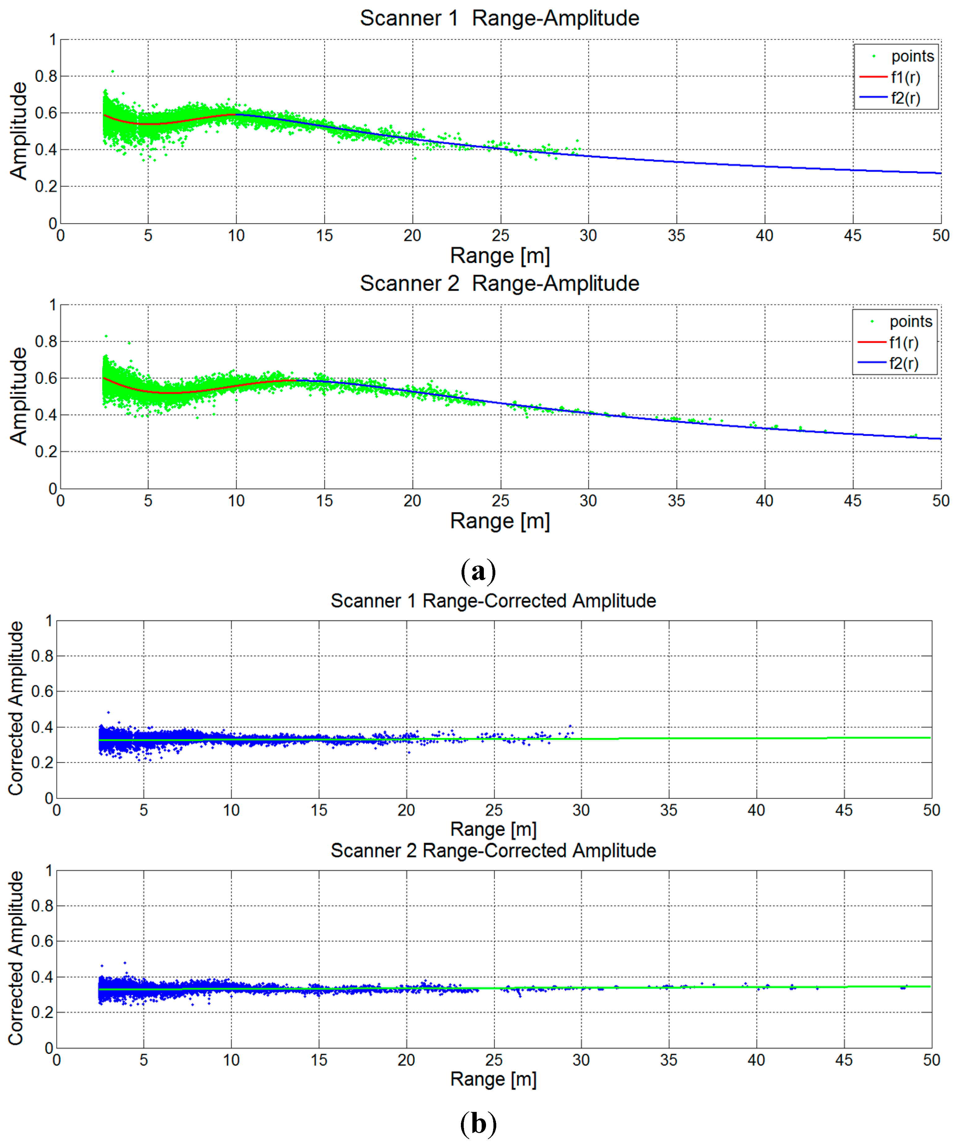
In the polynomial fitting for combination 3 (Figure 8), the red and blue lines were the polynomial functions for near-range and far-range. The behavior at near-range was not proportional to 1/r; therefore, a third-order range polynomial function was applied. After the near-range, a second-order 1/r polynomial function was used to ensure that the amplitude was decreasing while the range was increasing. Once the polynomial coefficients were calculated, we used polynomial function as a normalization factor and applied it to the original data (Figure 8a). After the range normalization, the relationship between range and corrected amplitude was evaluated (Figure 8b). The slope of normalized amplitude-range was near zero, demonstrating that the distance effect for asphalt road was removed via radiometric normalization.

Figure 8. Range-amplitude polynomial function (combination 3): (a) polynomial fitting and (b) amplitude normalization.

Figure 8. Range-amplitude polynomial function (combination 3): (a) polynomial fitting and (b) amplitude normalization.

4.2. Statistical Analysis

The evaluation process was introduced in Section 3.3.1, and here we show the quantitative results of radiometric normalization. The statistical analyses of amplitude difference were divided into delta amplitude between scanners and delta amplitude between strips to compare the differences between scanners and strips in overlapped areas (Table 3). The quantitative results included mean, standard deviation, and improvement (Equation (7)). The number of overlapped cells referred to the number of observations, and the cell size was 0.01 m². A large number of overlapped areas were selected in the evaluation process, which included a minimum number of observations of 140,000 cells.

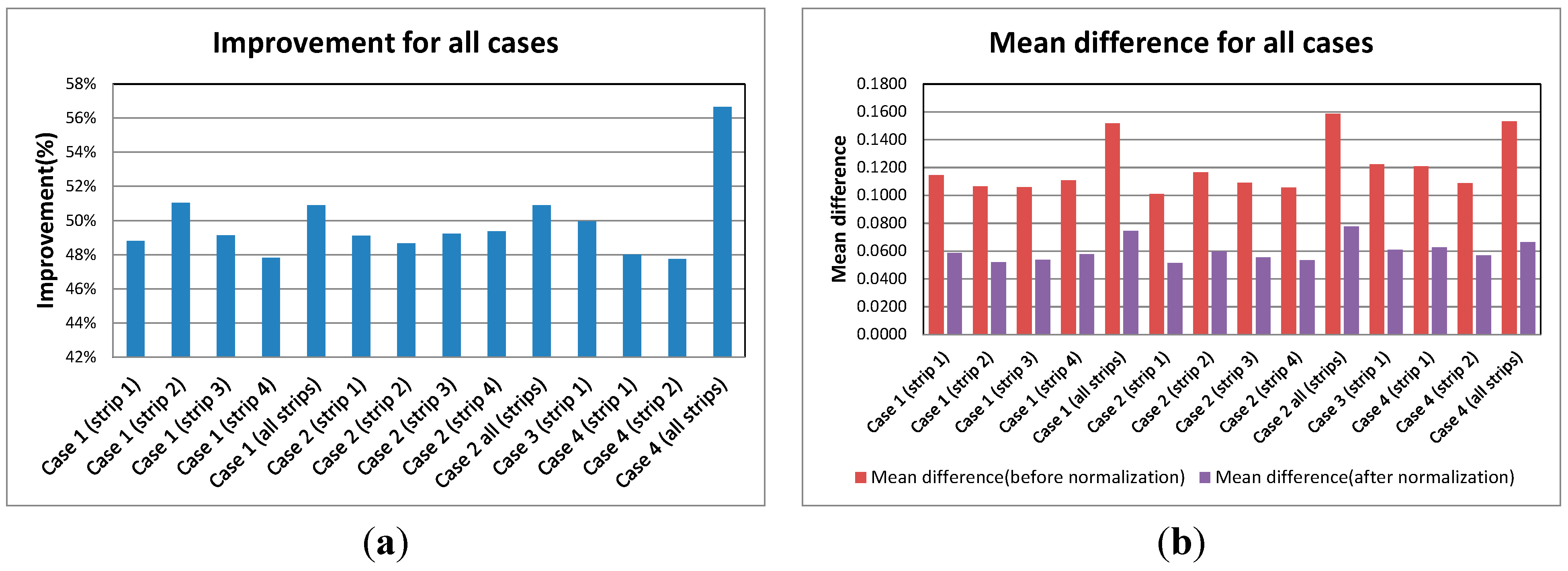
We used case 1 to calculate the normalization functions and apply to other cases. The developed radiometric normalization method was applied to all road points. In all cases, the mean and standard deviation of delta amplitude were reduced after the normalization. To compare the improvement for all cases (Figure 9a), the improvements ranged from 47% to 56%. The proposed method was suitable to improve the radiometric consistence from different strips and scanners, but most of the improvements between strips were higher than improvements between scanners. This study demonstrated that a standard area can be selected to obtain the normalization function and apply it to all dataset. Because crossroads usually contain multiple strips for more overlapped areas, we suggest using a crossroad as a standard area.

Table 3. Quantitative results for radiometric normalization.

			Number of Overlapped Cell	Original		Normalized		Improvement (%)
				Mean	Std.	Mean	Std.
Case 1	Between scanners	Strip 1	159,869	0.1145	0.0616	0.0586	0.0340	48.82%
		Strip 2	196,738	0.1063	0.0560	0.0520	0.0315	51.04%
		Strip 3	198,458	0.1058	0.0590	0.0538	0.0332	49.15%
		Strip 4	194,938	0.1106	0.0665	0.0577	0.0370	47.83%
	Between strips		322,272	0.1517	0.0576	0.0745	0.0328	50.89%
Case 2	Between scanners	Strip 1	145,301	0.1010	0.0602	0.0514	0.0326	49.11%
		Strip 2	150,302	0.1165	0.0611	0.0598	0.0339	48.67%
		Strip 3	145,162	0.1091	0.0588	0.0554	0.0331	49.22%
		Strip 4	150,035	0.1055	0.0581	0.0534	0.0322	49.38%
	Between strips		284,262	0.1585	0.0533	0.0778	0.0304	50.91%
Case 3	Between scanners	Strip 1	161,140	0.1221	0.0616	0.0611	0.0347	49.96%
Case 4	Between scanners	Strip 1	1,487,061	0.1208	0.0648	0.0628	0.0356	48.01%
		Strip 2	1,666,863	0.1087	0.0603	0.0568	0.0325	47.75%
	Between strips		586,934	0.1529	0.0748	0.0663	0.0354	56.64%

Table 3. Quantitative results for radiometric normalization.

			Number of Overlapped Cell	Original		Normalized		Improvement (%)
				Mean	Std.	Mean	Std.
Case 1	Between scanners	Strip 1	159,869	0.1145	0.0616	0.0586	0.0340	48.82%
		Strip 2	196,738	0.1063	0.0560	0.0520	0.0315	51.04%
		Strip 3	198,458	0.1058	0.0590	0.0538	0.0332	49.15%
		Strip 4	194,938	0.1106	0.0665	0.0577	0.0370	47.83%
	Between strips		322,272	0.1517	0.0576	0.0745	0.0328	50.89%
Case 2	Between scanners	Strip 1	145,301	0.1010	0.0602	0.0514	0.0326	49.11%
		Strip 2	150,302	0.1165	0.0611	0.0598	0.0339	48.67%
		Strip 3	145,162	0.1091	0.0588	0.0554	0.0331	49.22%
		Strip 4	150,035	0.1055	0.0581	0.0534	0.0322	49.38%
	Between strips		284,262	0.1585	0.0533	0.0778	0.0304	50.91%
Case 3	Between scanners	Strip 1	161,140	0.1221	0.0616	0.0611	0.0347	49.96%
Case 4	Between scanners	Strip 1	1,487,061	0.1208	0.0648	0.0628	0.0356	48.01%
		Strip 2	1,666,863	0.1087	0.0603	0.0568	0.0325	47.75%
	Between strips		586,934	0.1529	0.0748	0.0663	0.0354	56.64%

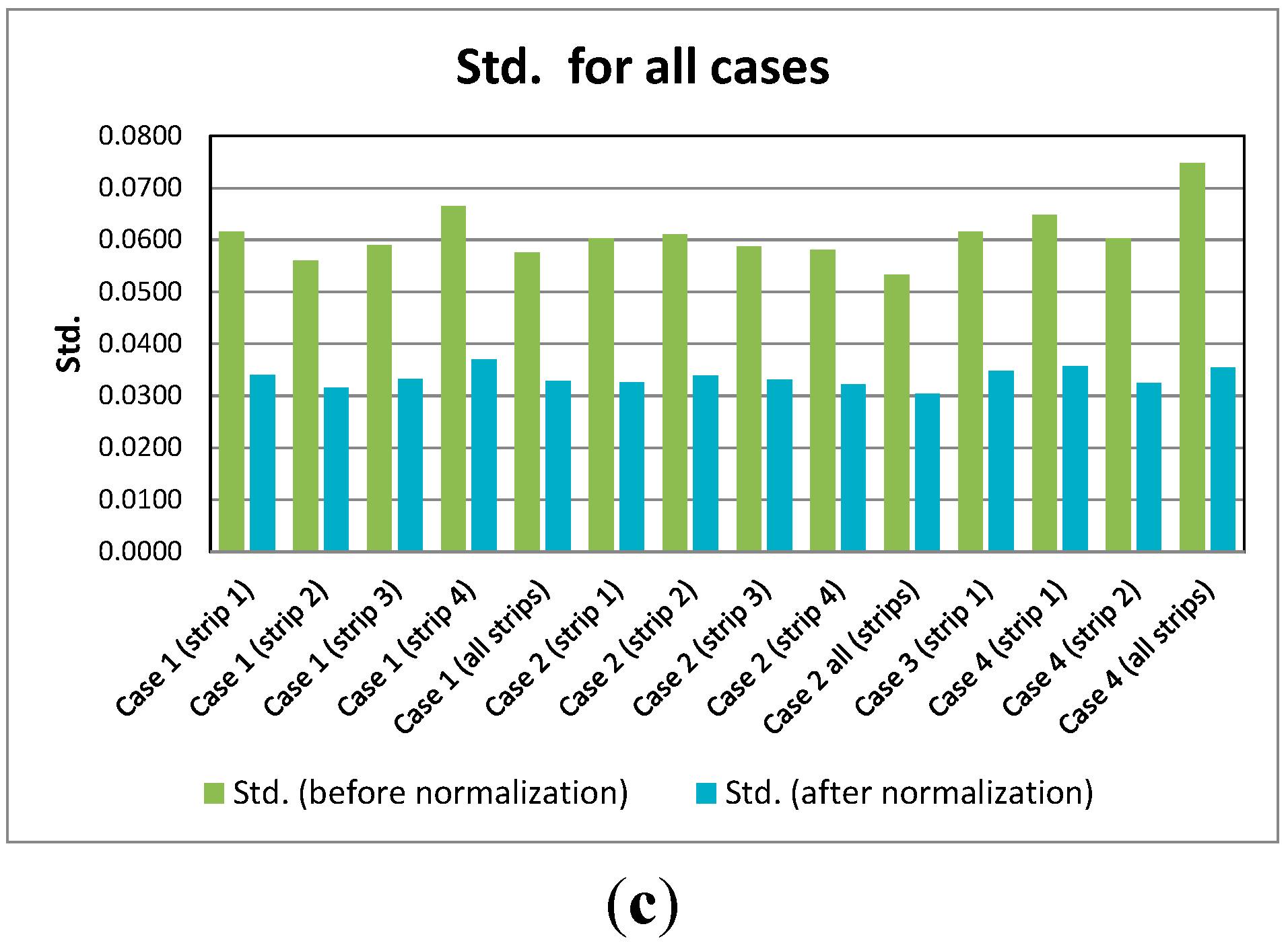
To compare the mean difference between scanners and strips (Figure 9b), the mean difference between strips was reduced from 0.15 to 0.07 while the mean difference between scanners was reduced from 0.10 to 0.06. Before normalization, the mean difference between strips was larger than the mean difference between scanners. For an overlapped area, the laser pulse from different strips had a larger difference than that from different scanners; therefore, radiometric normalization from different strips or different stations must be considered before application. The standard deviation of amplitude difference (Figure 9c) was reduced from 0.06 to 0.03, which was much lower than the mean difference. Because the results after normalization were similar to the fitting errors (RMSEs; Table 2), the remaining variations can be explained as the variation of road surface properties.

Figure 9. Comparison of statical results for all cases: (a) improvement, (b) comparison of mean differences, and (c) comparison of std. errors.

Figure 9. Comparison of statical results for all cases: (a) improvement, (b) comparison of mean differences, and (c) comparison of std. errors.

4.3. Road Surface Classification

The performance of road surface classification before and after radiometric normalization was analyzed. Theoretically, the painted colored road markings should have the highest amplitude, and the new asphalt pavement should have the lowest amplitude [36]. We used MLS amplitudes to separate ordinary asphalt road points, new pavement asphalt road points, and colored road marks via ISODATA unsupervised classification. Note that only amplitude was applied in road surface classification.

The confusion matrix was generated from a manually digitized road map for all four cases (Figure 10d, Figure 11d, Figure 12d and Figure 13g). Different colors indicated different types of road surfaces. Both original (Figure 10e, Figure 11e, Figure 12e and Figure 13h) and normalized (Figure 10f, Figure 11f, Figure 12f and Figure 13i) amplitudes were used in road surface classification (Table 4). The accuracy of classification after the normalization was higher than the original, indicating that the normalization increased the correctness in classification accuracy from 6% to 14%. In particular, the accuracy of new pavement was most significant.

Table 4. Summary of road surface classification.

Case		Correctness (%)			Completeness (%)			Overall Accuracy (%)	Kappa
		New Pavement	Ordinary Pavement	Road Mark	New Pavement	Ordinary Pavement	Road Mark
1	Original (ISODATA)	75.09	77.84	66.01	59.27	84.25	86.53	76.01	0.5422
	Normalized (ISODATA)	85.36	82.38	71.95	67.80	90.03	86.40	82.29	0.6597
	Normalized (OBC)	81.69	88.16	76.20	81.68	87.50	81.00	85.08	0.7200
2	Original (ISODATA)	59.26	80.25	80.72	64.28	76.45	83.90	73.31	0.4985
	Normalized (ISODATA)	85.18	90.23	77.09	80.3	90.9	89.77	87.56	0.7626
	Normalized (OBC)	93.43	91.71	65.46	80.86	93.08	91.91	89.24	0.7960
3	Original (ISODATA)	58.58	68.96	25.13	44.38	65.74	84.31	59.47	0.2531
	Normalized (ISODATA)	69.56	76.99	37.92	57.18	77.32	84.12	70.90	0.4388
	Normalized (OBC)	68.79	81.10	59.98	70.51	78.97	69.45	75.61	0.5260
4	Original (ISODATA)	3.68	98.89	37.61	69.44	84.18	85.1	84.17	0.3358
	Normalized (ISODATA)	8.66	98.85	40.06	48.82	90.48	85.13	90.02	0.4521
	Normalized (OBC)	61.31	98.70	52.26	66.69	95.57	80.64	94.64	0.6090

Table 4. Summary of road surface classification.

Case		Correctness (%)			Completeness (%)			Overall Accuracy (%)	Kappa
		New Pavement	Ordinary Pavement	Road Mark	New Pavement	Ordinary Pavement	Road Mark
1	Original (ISODATA)	75.09	77.84	66.01	59.27	84.25	86.53	76.01	0.5422
	Normalized (ISODATA)	85.36	82.38	71.95	67.80	90.03	86.40	82.29	0.6597
	Normalized (OBC)	81.69	88.16	76.20	81.68	87.50	81.00	85.08	0.7200
2	Original (ISODATA)	59.26	80.25	80.72	64.28	76.45	83.90	73.31	0.4985
	Normalized (ISODATA)	85.18	90.23	77.09	80.3	90.9	89.77	87.56	0.7626
	Normalized (OBC)	93.43	91.71	65.46	80.86	93.08	91.91	89.24	0.7960
3	Original (ISODATA)	58.58	68.96	25.13	44.38	65.74	84.31	59.47	0.2531
	Normalized (ISODATA)	69.56	76.99	37.92	57.18	77.32	84.12	70.90	0.4388
	Normalized (OBC)	68.79	81.10	59.98	70.51	78.97	69.45	75.61	0.5260
4	Original (ISODATA)	3.68	98.89	37.61	69.44	84.18	85.1	84.17	0.3358
	Normalized (ISODATA)	8.66	98.85	40.06	48.82	90.48	85.13	90.02	0.4521
	Normalized (OBC)	61.31	98.70	52.26	66.69	95.57	80.64	94.64	0.6090

For the regions near to the trajectory, the data set without normalization shows higher amplitude than the normalized data. Without the radiometric normalization, the amplitude of new pavement near to the trajectories is higher than the new pavement distributed on other regions. Consequently, the new pavement near to the trajectory is easily misclassified into ordinary pavement. After the normalization, the new pavement at different locations has similar amplitude and can be classified correctly. For the ordinary pavement distributed on far-range regions, the data set without normalization shows lower amplitude when compared to ordinary pavement distributed on near-range regions. In other words, the same pavement distributed at different locations has large amplitude differences. Some of the far-range ordinary pavement has amplitude similar to near-range new pavement. Therefore, the far-range ordinary pavement might be misclassified into new pavement. After the normalization, the ordinary pavement at different locations has similar amplitude and can be classified correctly. The experimental results indicated that the normalized amplitudes can be used to separate new and old pavements.

To compare the results of ISODATA from original and normalized amplitudes, the overall accuracies of cases 1 and 2 were higher than the other cases as the number of strips for the first two cases is larger than cases 3 and 4. Although the overall accuracies for cases 3 and 4 were greater than 70%, the Kappas were less than 0.5 because the majority of road surface was ordinary asphalt road. Because the ordinary pavement of case 4 was covered by a serious tire footprint, the correctness of new pavement in case 4 was less than 10%. The area of new pavement (i.e., 12.76 m²) in case 4 was relatively smaller than other cases. The commission areas for original and normalized amplitude were 231.71 m² and 65.68 m², respectively, and the result of normalized amplitude was better than original amplitude.

To compare the results of point-based (ISODATA) and object-based classification (OBC) for normalized amplitudes, the object-based classification provides higher accuracy than ISODATA in all cases (see Table 4). The results of object-based classification are shown as Figure 10g, Figure 11g, Figure 12g and Figure 13j. The object-based classification aggregates the points with similar amplitude into regions, then, it separates different road surfaces based on amplitudes of regions. The improvement of overall accuracy ranged from 1.68% to 4.62% while the improvement of Kappa ranged from 0.033 to 0.156. This object-based classification improves the salt-and-pepper effect when utilizing the lidar amplitude in classification. The object-based classification significantly improved the accuracy of ISODATA in Case 4. The overall accuracy and Kappa reached 94.64% and 0.6090, respectively, in Case 4.

4.4. Visualization Check

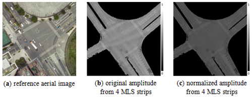
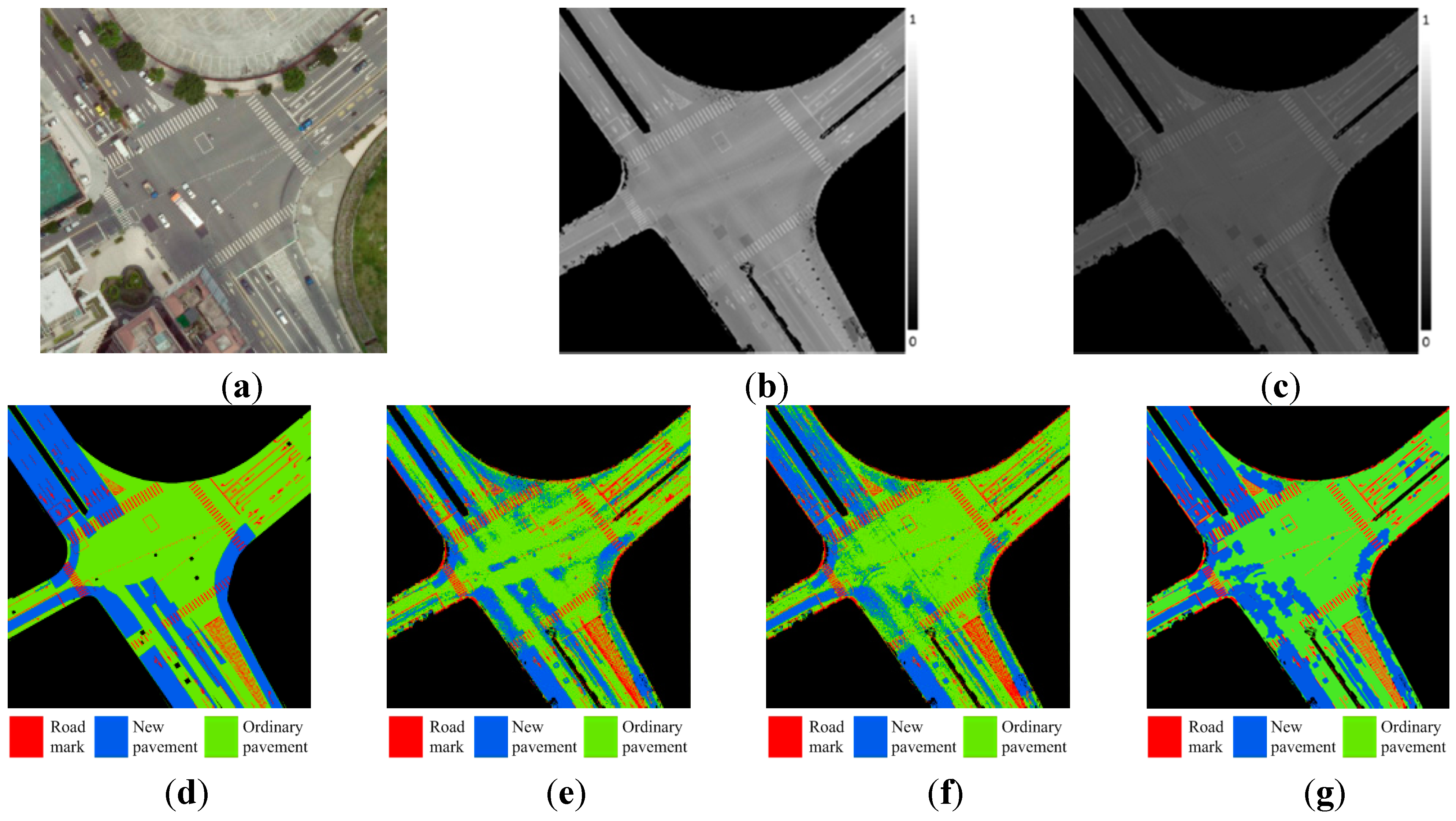
After the numerical analysis, we visually compared MLS before and after radiometric normalization for case 1 using aerial orthophoto (Figure 10a). From the amplitude of road points before and after normalization (Figure 10b,c), it can be seen that the original amplitude image has high amplitude along the trajectory, but this phenomenon did not occur in the reference orthophoto; the radiometrical discrepancy was removed after normalization (Figure 10c). From the manual digitization (Figure 10d) and the results of unsupervised classification before and after normalization (Figure 10e,f), it can be seen that original classification result and manual digitization were different. Although the new pavements were misclassified into ordinary pavement at near range, the classification was improved after the range normalization.

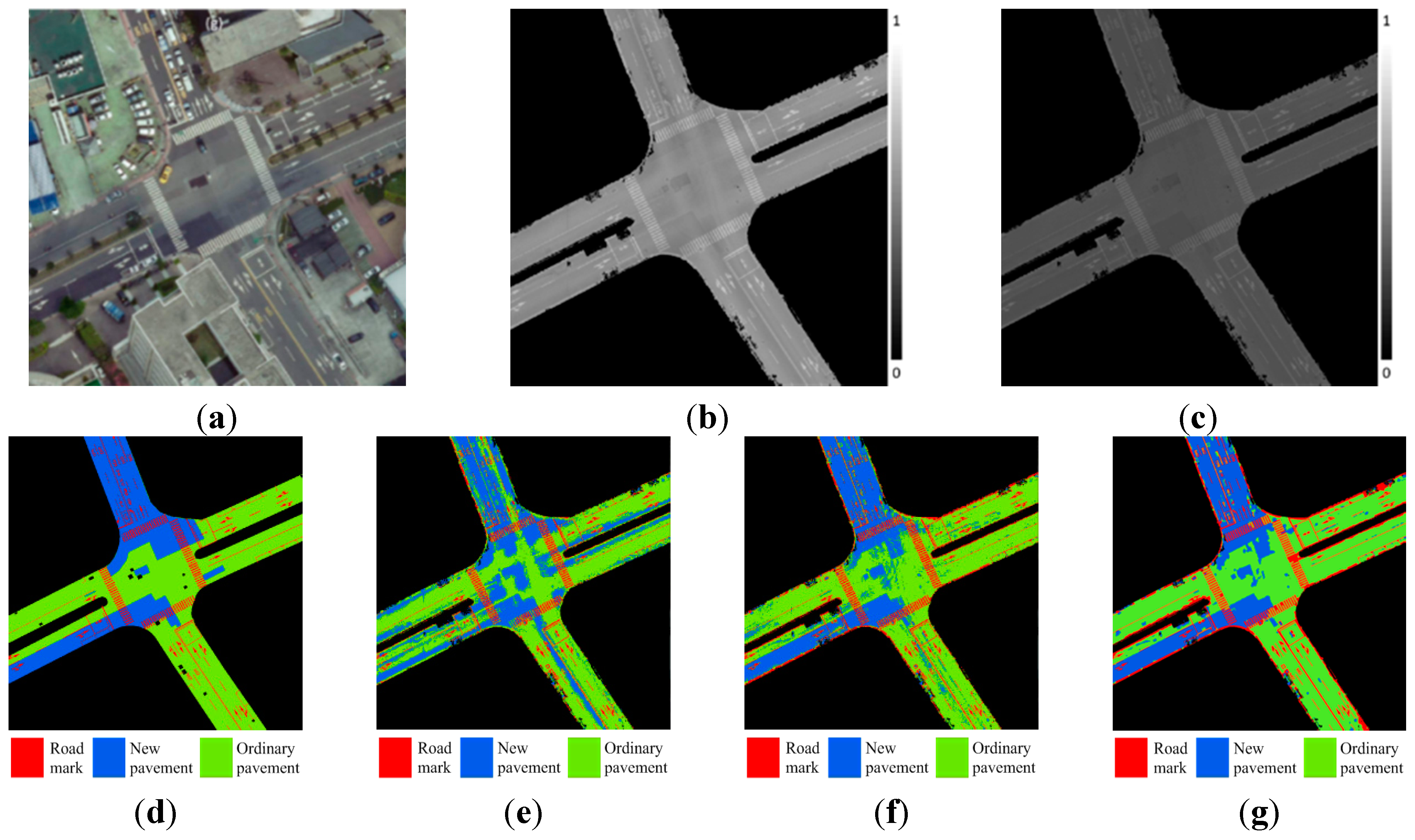
At the case 2 crossroad, an aerial orthoimage (Figure 11a) was included for comparison. This area covered a large area of new asphalt pavement and showed the original and normalized amplitudes (Figure 11b,c, respectively). The near-range effect of MLS was removed after the radiometric normalization, and the coverage of new asphalt pavement was clearer in the normalized amplitude image (Figure 11c) than the original (Figure 11b). The classification results also showed that the road surface can be classified correctly after the range normalization (Figure 11d–f).

Figure 10. Case 1: (a) orthophoto, (b) original amplitude, (c) corrected amplitude, (d) manual digitization, (e) classified results using original amplitude, (f) classified results using corrected amplitude, and (g) results of object-based classification using corrected amplitude.

Figure 10. Case 1: (a) orthophoto, (b) original amplitude, (c) corrected amplitude, (d) manual digitization, (e) classified results using original amplitude, (f) classified results using corrected amplitude, and (g) results of object-based classification using corrected amplitude.

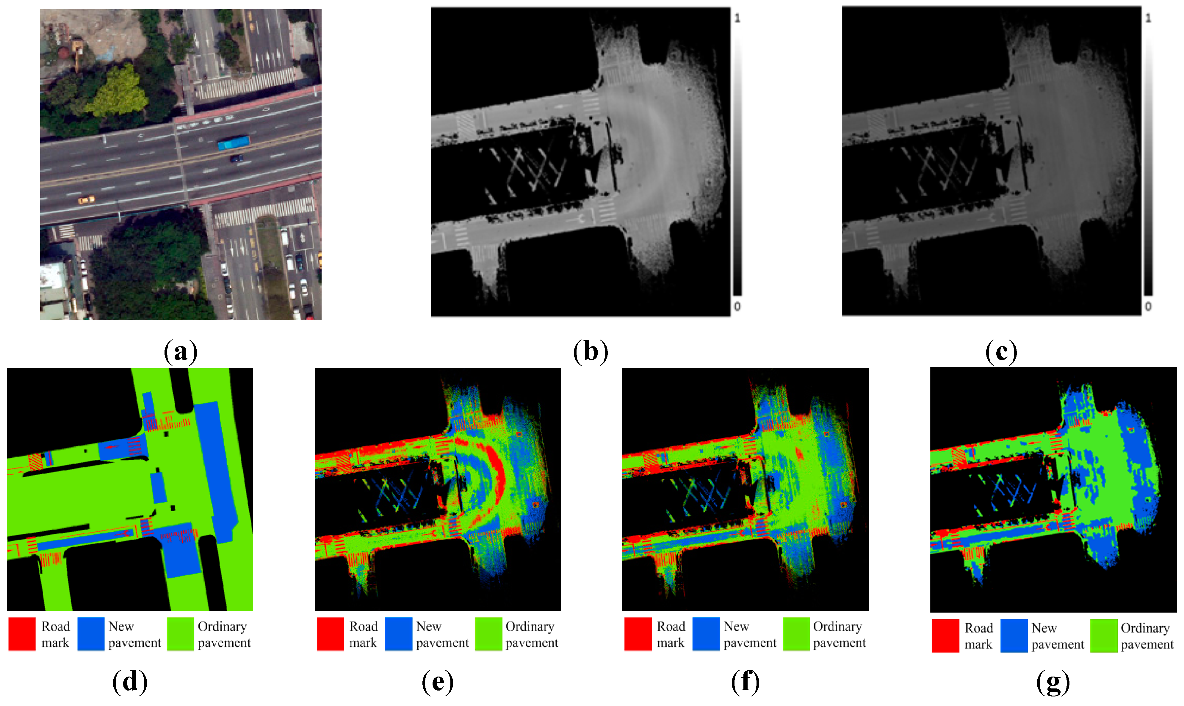
The case 3 U-turn road covered an underpass road section, and the corresponding aerial orthophoto (Figure 12a) covered the high-pass road. Because most of the road surfaces in case 3 were occluded by the high-pass road and trees in the aerial orthophoto, this case demonstrated the possibility of obtaining an underpass road surface from MLS, which is more suitable than aerial photography for monitoring the road surface in an underpass environment. Only one strip showed the amplitude before and after normalization (Figure 12b,c); however, the near-range effect of this dual-laser system produced higher amplitudes near to the trajectory (Figure 12b). This phenomenon could be normalized via the proposed method (Figure 12c), meaning that the MLS should be corrected even though it only has one strip. The reference road surface map (Figure 12d) and the unsupervised classification of original and range-corrected amplitude images (Figure 12e,f) show that the original amplitude image incorrectly classifies the new pavement as old pavement, but the range-corrected amplitude image corrects the classification. The experimental result also showed the improvement in road surface classification.

Figure 11. Case 2: (a) orthophoto (reference only), (b) original amplitude, (c) corrected amplitude, (d) manual digitization, (e) classified results using original amplitude, (f) classified results using corrected amplitude, and (g) results of object-based classification using corrected amplitude.

Figure 11. Case 2: (a) orthophoto (reference only), (b) original amplitude, (c) corrected amplitude, (d) manual digitization, (e) classified results using original amplitude, (f) classified results using corrected amplitude, and (g) results of object-based classification using corrected amplitude.

Figure 12. Case 3 (underway lidar acquisition): (a) aerial photo above the underpass, (b) original amplitude, (c) corrected amplitude, (d) manual digitization, (e) classified results using original amplitude, (f) classified results using corrected amplitude, and (g) results of object-based classification using corrected amplitude.

Figure 12. Case 3 (underway lidar acquisition): (a) aerial photo above the underpass, (b) original amplitude, (c) corrected amplitude, (d) manual digitization, (e) classified results using original amplitude, (f) classified results using corrected amplitude, and (g) results of object-based classification using corrected amplitude.

Case 4 included two opposite strips, 1.4 km in length. The amplitudes before and after normalization (Figure 13a,d) included two enlarged subareas for better observation of the original (Figure 13b,c) and normalized (Figure 13e,f) data. The near range effect was corrected after normalization. 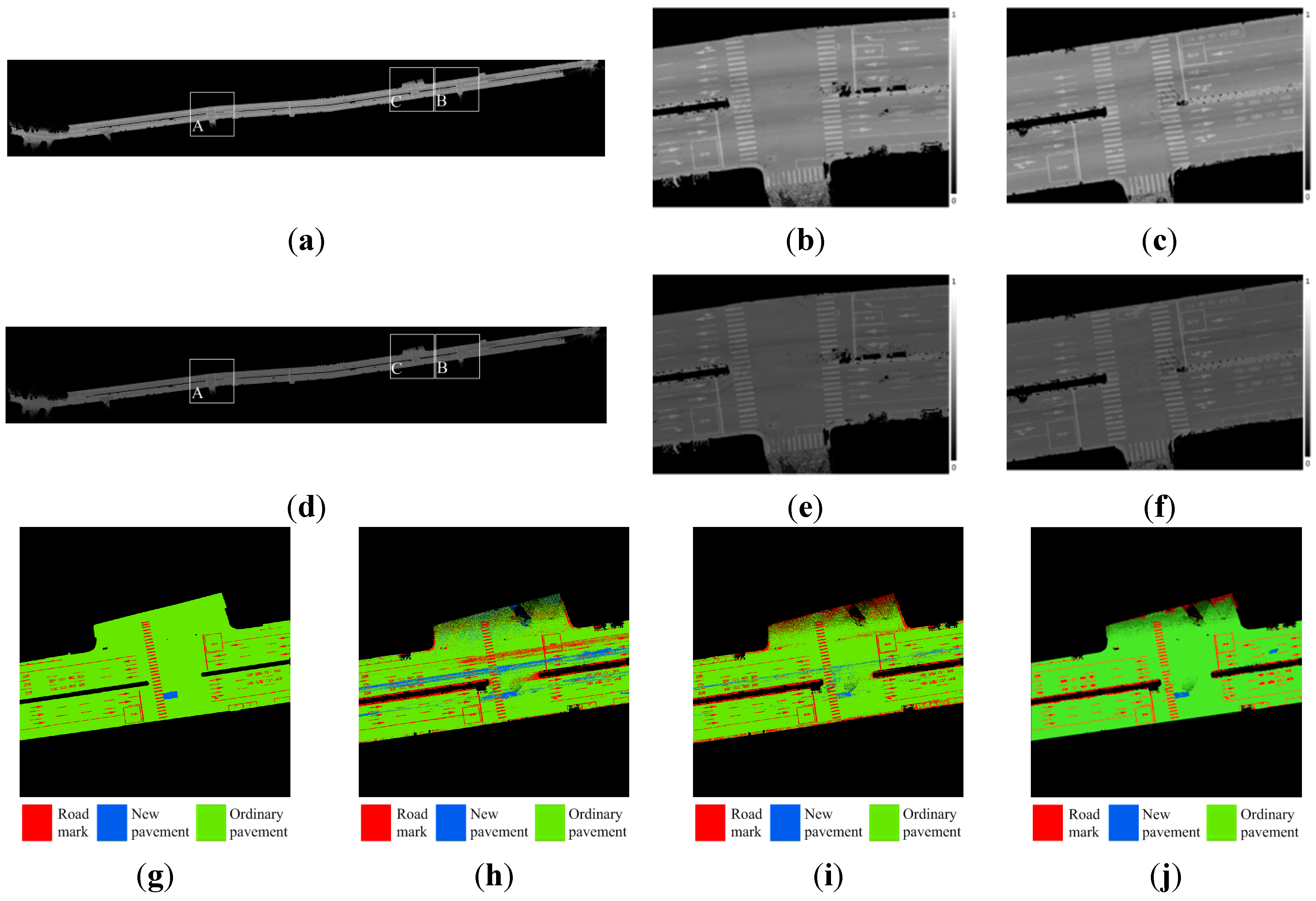The results demonstrate that the proposed method works well for longer strips for road surface classification (Figure 13g–i). Before normalization, the ordinary roads were significantly misclassified into new pavements and road markings, a phenomenon that can be improved by using the normalized amplitude.

Figure 13. Case 4: (a) original amplitude, (b) original amplitude (zoom-in A), (c) original amplitude (zoom-in B), (d) range-corrected amplitude, (e) range-corrected amplitude (zoom-in A), (f) range-corrected amplitude (zoom-in B), (g) manual digitization (zoom-in C), (h) classified results using original amplitude (zoom-in C), (i) classified results using range-corrected amplitude (zoom-in C), and (j) results of object-based classification using corrected amplitude (zoom-in C).

Figure 13. Case 4: (a) original amplitude, (b) original amplitude (zoom-in A), (c) original amplitude (zoom-in B), (d) range-corrected amplitude, (e) range-corrected amplitude (zoom-in A), (f) range-corrected amplitude (zoom-in B), (g) manual digitization (zoom-in C), (h) classified results using original amplitude (zoom-in C), (i) classified results using range-corrected amplitude (zoom-in C), and (j) results of object-based classification using corrected amplitude (zoom-in C).

5. Conclusions

In this study, we proposed a range normalization method to reduce the abnormal amplitude phenomenon at near distance. We assumed that conjugate asphalt roads from different laser scanners or strips would have similar responses. The systematic error can be eliminated through the empirical function. The experimental results indicated that the proposed method may improve the radiometric consistency of road points between scanners and strips. Four different cases were evaluated. In the visual display, the amplitude became more consistent after normalization, and the abnormal amplitude phenomenon of the trajectory along the scanner was corrected. In the consistency check, the amplitude discrepancy was reduced via the proposed method. The improvements for amplitude consistency were better than 47% between scanners and 50% between strips. In the road surface classification, the accuracy of classification after the normalization was higher than the original, and the overall accuracy reached 70% for road surface classification. In particular, the improvement of new pavement was most significant. For the road surface classification, we were only concerned with the radiometric normalization for road points by natural signalized target. In future studies, the road surface classification should explore more variables than amplitude, the only one adopted in this study. Further improvements of classification should include additional lidar features [28].