An Improvement of the Radiative Transfer Model Component of a Land Data Assimilation System and Its Validation on Different Land Characteristics

Abstract

The paper reports the recent progress in the radiative transfer model (RTM) development, which serves as the observation operator of a Land Data Assimilation System (LDAS), and its validation at two Planetary Boundary Layer (PBL) stations with different weather and land cover conditions: Wenjiang station of humid and cropped field and Gaize station of arid and bare soil field. In situ observed micrometeorological data were used as the driven data of LDAS, in which AMSR-E brightness temperatures (TB) were assimilated into a land surface model (LSM). Near surface soil moisture content output from LDAS, together with the one simulated by a LSM with default parameters, were compared to the in-situ soil moisture observation. The comparison results successfully validated the capability of LDAS with new RTM to simulate near surface soil moisture at various environments, supporting that LDAS can generally simulate soil moisture with a reasonable accuracy for both humid vegetated fields and arid bare soil fields while the LSM overestimates near surface soil moisture for humid vegetated fields and underestimates soil moisture for arid bare soil fields.

1. Introduction

Surface soil moisture, which links the land surface and the atmosphere by influencing the exchange of energy and mass between the two [1], is one of the most important variables in much of the Earth system research, such as hydro-meteorological studies, global scale environmental processes monitoring and climate change studies [2,3].

Traditionally, in-situ near surface soil moisture is measured at points, by using conventional can-sampling method and/or using newly developed techniques such as Time Domain Reflectometry (TDR) and neutron probe. Through these methods, very accurate soil moisture profiles can be observed. However, due to the large spatial variability of soil moisture, it is very difficult to observe the spatial distribution of soil moisture over a large scale by such in-situ measurements, which are both time consuming and expensive.

Fortunately, satellite passive microwave remote sensing makes it possible to measure surface soil moisture at the global scale by direct measurement of brightness temperature which is strongly related to the liquid moisture content [4,5,6,7]. Researchers have developed several algorithms to retrieve soil moisture from brightness temperatures observed at various frequencies, polarizations, and viewing angles [4,8,9,10,11]. However, remotely sensed soil moisture content still contains large errors and needs to be improved greatly. Moreover, the spaceborne remote sensing generally only can provide a snap shot of the Earth’s surface. As a result, the near surface soil moisture observed by satellite therefore is discontinuous in time.

On the other hand, land surface models (LSMs) are able to predict temporal and spatial patterns of land surface variables [12,13]. Based on the complexity of model structure and parameter selection, LSMs can be generally divided into two categories: simplified LSMs and biophysically based LSMs. A simplified LSM usually uses a solution-based method to compute the exchanges of energy, water and moment between land and atmosphere [14]. A biophysically based LSM [13,15,16,17,18] generally simulates the exchanges through a process-based way for specific land cover, such as bare soil [19,20], frozen soil [21] and grassland [22]. On a local scale, with accurate meteorological forcing and carefully-calibrated parameters, both simplified and comprehensive ones can well simulate the land surface dynamic. When running the model on a large scale, the quality of the LSM predictions are usually not so good because of model initialization, parameter and forcing errors, and inadequate model physics and/or resolution [23,24].

The Land Data Assimilation System (LDAS), developed by merging observation information (from ground-based stations, satellites and so on) into dynamic models (i.e., LSMs), is expected to provide high quality surface energy and water flux estimates with adequate coverage and resolution [25,26]. The systems were developed based on field experiments for case studies [27,28], and then extended to regional scale, such as the North American Land Data Assimilation System (NLDAS) [29], and global scale, such as the Global Land Data Assimilation System (GLDAS) [30]. Since the data assimilation methods can consistently couple both modeling and observations, LDAS is able to yield superior land surface status [19,21,22]. Previous studies [25,27,31,32,33,34] have demonstrated that the assimilation product is superior to both satellite data and model data when these datasets are considered in isolation.

Yang et al. developed a dual-pass land data assimilation system at the University of Tokyo (LDAS-UT) [35]. It then has been further applied by Yang et al. [32] and Zhao et al. [36] over a Mongolian semiarid region, and by Lu et al. [31] and Zhao et al. [37] over the Tibetan Plateau. Recently, Rasmy et al. [38] has coupled LDAS-UT with an atmospheric model to improve the weather forecast in Africa. In these applications, the Radiative Transfer Model (RTM) inside LDAS-UT is the Q-H model [39,40], an empirical RTM mainly focusing on the surface scattering process at the land–air interface. In this study, we improved the RTM component by using a more physically-based one in which both the surface scattering process and volume scattering inside the soil layer are included.

The objective of this study is to evaluate the new LDAS-UT in different climate and land cover conditions. LDAS-UT was applied at two Planetary Boundary Layer (PBL) tower stations with different climate and land cover conditions: the Wenjiang station which is humid and located in a vegetated field; and the Gaize station which is arid and located in a bare soil field. In order to evaluate our system, the output of LDAS-UT was compared with in-situ soil moisture observation. We also compared the soil moisture simulated by LSM with the in-situ observed ones, to confirm the advantages of LDAS-UT.

In the following section, we briefly introduce the LDAS-UT, with emphasis on the newly extended RTM, in which the volume scattering effects of dry soil media and the surface scattering effects of rough surface are physically represented and coupled. The materials and methods used in this study, including the two PBL stations, meteorological forcing data and statistical equations, are also described in Section 2. The simulation results of LDAS-UT at two stations are described in Section 3. Finally, we finish this paper with some conclusions.

2. LDAS, Data and Method

2.1. Land Data Assimilation System of the University of Tokyo (LDAS-UT)

LDAS-UT was designed to assimilate the satellite remotely sensed microwave brightness temperature data into LSM, to improve the estimate of soil moisture status and then to improve the simulation of land surface energy and water budget. The satellite observation data used in this study is the low frequencies (6.9 GHz and 18.7 GHz vertical polarization) observation of the Advanced Microwave Scanning Radiometers for EOS (AMSR-E).

2.1.1. Three Components of LDAS-UT

The LDAS-UT consists of a LSM to update the land surface status and calculate surface fluxes, a RTM to simulate microwave brightness temperature for corresponding land surface status, and an optimization scheme to search for optimal values of soil moisture by minimizing the difference between simulated and observed brightness temperature.

The LSM is the Simple Biosphere model (SiB2) [13,41], with some modifications to the heat and momentum transfer simulation for bare soil [42] and for sparse canopy [43]. The information observed by AMSR-E was assimilated into the surface layer soil moisture with a variational method.

The minimization scheme is Shuffled Complex Evolution (SCE) method [44]. The detail of the LSM can be found in [35]. In this paper, we will mainly introduce the new progress made in the RTM part of LDAS-UT.

2.1.2. Development in Observation Operator: Extended RTM

In this research, in order to simulate the radiative process inside the dry soil media accurately, we extended the RTM to include the volume scattering effects of dry soil particles and the influence of moisture and temperature profile. The empirical surface roughness model used in former RTM was also replaced by a sophisticated physical-based model, Advanced Integral Equation Method (AIEM) [45].

In current RTM, the downward radiation from vegetation and atmosphere, which are reflected by soil surface, is neglected considering the fact that the reflection at the soil surface is much smaller than the emission from the surface. Furthermore, as the atmosphere is almost transparent for the low frequencies of microwave region (less than 18GHz), the brightness temperature observed by spaceborne sensors is then expressed as:

$$T_b=T_{bs}{e}^{-{\tau }_c}{e}^{-{\tau }_r}+(1-{\omega }_c)(1-e^{-{\tau }_c})T_c{e}^{-{\tau }_r}$$

(1)

where T_bs is the emission of soil layer, T_c is the vegetation temperature, T_r is the temperature of precipitation droplets, τ_c and ω_c are the vegetation opacity and single scattering albedo.

The emission from soil is controlled by the soil properties and land surface roughness. Soil properties, such as soil temperature, moisture content, and texture profiles, are taken into account through dielectric constant models and radiative transfer process inside the soil media. In our RTM, the Dobson model [46,47] is used to calculate the dielectric constant of soil; and the radiative transfer process inside the soil is simulated by a discrete ordinate method as proposed by [48], with assumptions that the soil has a multi-layer structure and is composed of many plane-parallel and azimuthally symmetric soil slabs with spherical scattering particles.

$$\mu \frac{d}{d\tau }\left[\begin{array}{c}{I}_v(\tau ,\mu )\\ I_h(\tau ,\mu )\end{array}\right]=\left[\begin{array}{c}{I}_v(\tau ,\mu )\\ I_h(\tau ,\mu )\end{array}\right]-(1-{\omega }_0)B(\tau )\left[\begin{array}{c}1\\ 1\end{array}\right]-\frac{{\omega }_0}{2}{\displaystyle \underset{-1}{\overset{1}{\int }}\left[\begin{array}{cc}{P}_{VV}& P_{VH}\\ P_{HV}& P_{HH}\end{array}\right]}\left[\begin{array}{c}{I}_v(\tau ,{\mu }^{\prime })\\ I_h(\tau ,{\mu }^{\prime })\end{array}\right]d{\mu }^{\prime }$$

(2)

where, I_P(τ,μ) is the radiance at optical depth τ (dτ=K_edz, with extinction coefficient K_e and layer thickness dz) in direction μ for polarization status P (horizontal or vertical), ω₀ is the single scattering albedo of soil particle, B(τ) is the Plank function and P_ij (i,j=H or V) is the scattering phase function. The four-stream model proposed by [49] solves Equation (2) by using the discrete ordinate method and introducing the approximations that no cross-polarization exists. The Henyey-Greenstein formula [50] is used to express the scattering phase function of Equation (2).

For each slab, the extinction coefficient K_e and albedo ω used in Equation (1) were calculated by the so-called dense media radiative transfer theory (DMRT) under the Quasi Crystalline Approximation with Coherent Potential (QCA-CP) [51,52].

Land surface roughness effect is simulated by the Advanced Integral Equation Model (AIEM). AIEM is a physically based model, with only two parameters: standard deviation of the height variations σ (or rms height) and the surface correlation length l. AIEM is extended from the integral Equation Model (IEM) [53], which has demonstrated that IEM has a much wider application range for surface roughness conditions than the other models such as the Small Perturbation Model (SPM), Physical Optics Model (POM) and Geometric Optics Model (GOM). Compared with IEM, AIEM improves the calculation accuracy of the scattering coefficient by keeping the absolute phase term in Greens function which was neglected by IEM.

By coupling AIEM with DMRT, this radiative transfer model for soil media is a fully physically based model, hereinafter termed as DMRT-AIEM model. As a fully physically based radiative transfer model, the parameters of DMRT-AIEM, such as the RMS height, correlation length and soil particle size, have clearly physical meaning and their values can be obtained from field measurement or theoretical calculation.

The soil emission T_bs shown in Equation (1) is calculated by DMRT-AIEM in the following steps:

(i)

soil layer is divided into several slabs, which have the same thickness (dz). The temperature and soil moisture of each slab is interpolated from SiB2 simulation.

(ii)

The radiance is integrated from the bottom layer to the uppermost layer, by using Equation (2) and DMRT. By using Plank function, the radiance is converted to the apparent temperature.

(iii)

The emissivity of soil layer is calculated by AIEM.

(iv)

Finally, by multiplying apparent temperature with the emissivity, soil emission T_bs is calculated.

As shown in Equation (1), the effects of a vegetation layer depends on the vegetation opacity τ_c and the single scattering albedo of vegetation ω_c. The vegetation opacity in turn is strongly affected by the vegetation columnar water content W_c, the relationship can be expressed as [54]:

$${\tau }_c=\frac{b^{\prime }{\lambda }^{\chi }{W}_c}{\cos \mathrm{\theta }}$$

(3)

where λ is the wavelength; θ is the incident angle; χ and b′ are coefficients dependent on the vegetation type and structure; W_c is the vegetation water content (kg∙m⁻²), estimated from the Leaf Area Index (LAI) (m²∙m⁻²) using the relationship proposed by [55]:

$$W_c=\exp (LAI/3.3)-1$$

(4)

The single scattering albedo of vegetation ω_c is small at low frequency region of microwave [55]. In this research, the ω_c is calculated by

$${\omega }_c={\omega }_0\cdot \sqrt{W_c}$$

(5)

where ω_c is empirical coefficient, depending on vegetation geometry.

2.1.3. Dual-Pass Run Algorithm and Parameters

LDAS-UT adopts a dual-pass assimilation technique to solve parameterization problems. Pass 1 inversely estimates the optimal values of model parameters with long-term (~months) forcing data and brightness temperature data, and Pass 2 only estimates the near-surface soil moisture in a daily assimilation cycle. The details of the algorithm can be found in Figure 1 of Yang et al. [35]. A brief summary of the algorithm is given here for convenience, as follows:

(1)

LDAS-UT is a variational assimilation system, while its cost function is minimized by SCE;

(2)

Radiance (brightness temperature) is directly assimilated into LSM (SiB2) by updating surface soil moisture values;

(3)

Soil parameters used in LSM and RTM are first optimized in Pass 1, which run continuously for a period of around three months. The cost function of parameter optimization is shown in Equation (6), as:

$$COST={\displaystyle \sum _{i=1}^n{\displaystyle \sum _{j=1}^2{[T{B}_{obs,i}(f_j,p)-T{B}_{sim,i}(f_j,p)]}^2}}$$

(6)

where n is the number of AMSR-E observation during the optimization window; obs represents the observed brightness temperature by AMSR-E; sim represents the simulated brightness temperature by RTM; f is the frequency, f₁ = 6.925 GHz, f₂ = 18.7 GHz; p is the polarization. Through minimizing the cost, the parameter sets are optimized. The optimized parameters in Pass 1 are soil porosity, soil texture (percentage of sand and clay), surface roughness parameters (r.m.s height and correlation length), vegetation RTM parameters (χ and b′).

(4)

Soil moisture status in LSM is updated at the initial time of each assimilation cycle (~1 day), through minimizing the cost function of assimilation pass, as Equation (3) in Yang et al. (2007b):

$$COST={\displaystyle \sum _{j=1}^2\{{[T{B}_{obs}(f_j,p)-T{B}_{sim}(f_j,p)]}^2}+{[T{B}_0(f_j,p)-T{B}_{0,bg}(f_j,p)]}^2\}$$

(7)

where TB₀ and B_0,bg are the simulated brightness temperature using renewed soil moisture and the background soil moisture, respectively.

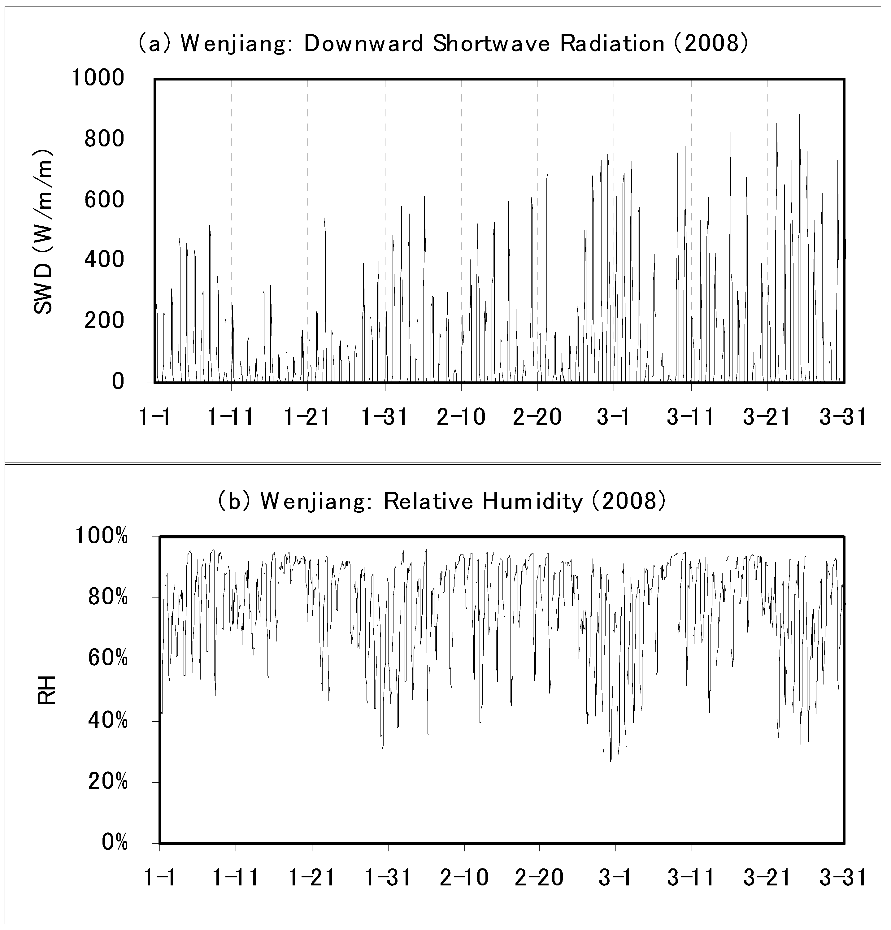
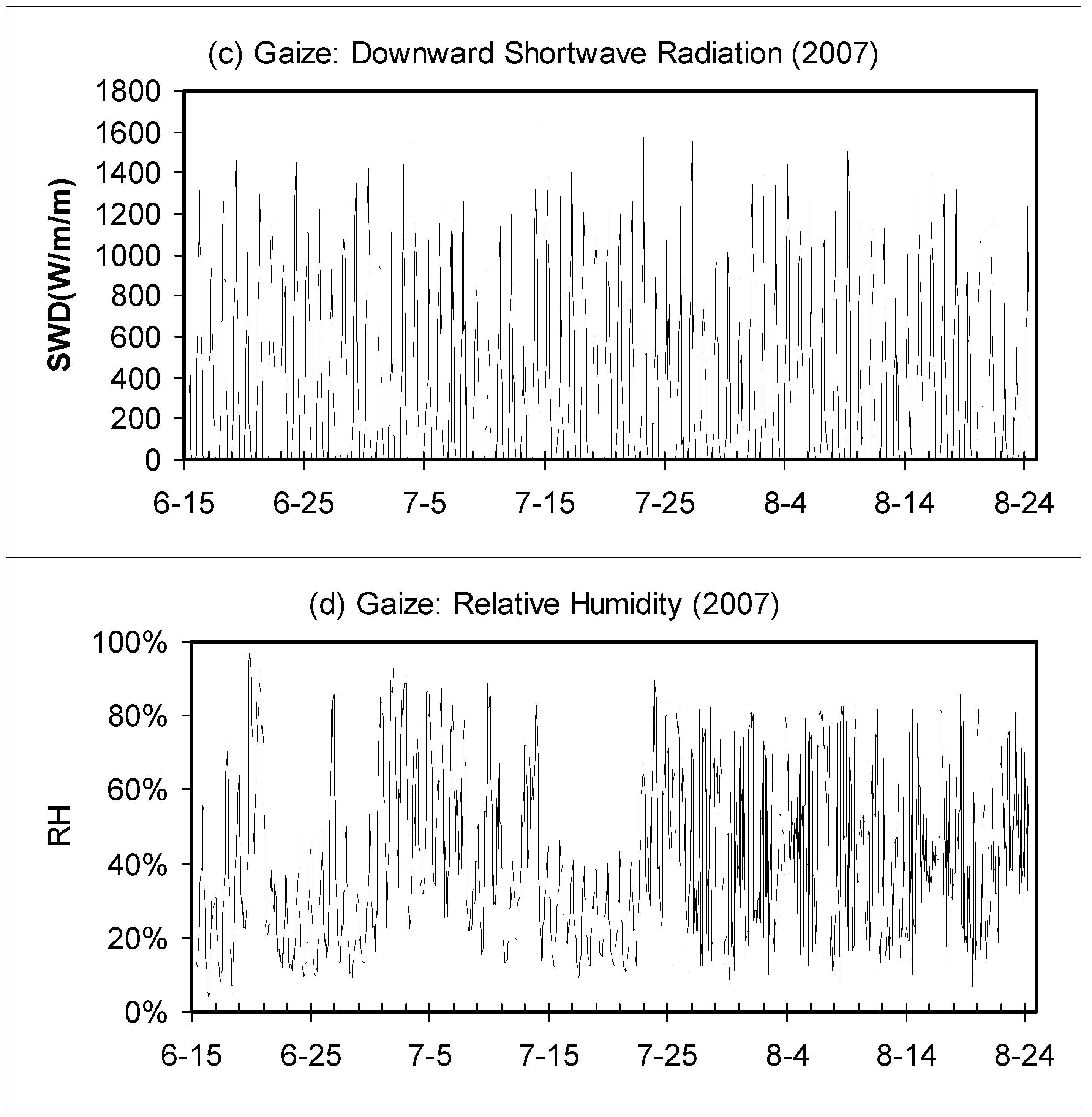
Figure 1. Meteorological forcing components: downward shortwave radiation (W/m²) at Wenjiang (a) and Gaize (b); relative humidity at Wenjiang (c) and Gaize (d).

Figure 1. Meteorological forcing components: downward shortwave radiation (W/m²) at Wenjiang (a) and Gaize (b); relative humidity at Wenjiang (c) and Gaize (d).

2.2. PBL Site: Wenjiang and Gaize

The Wenjiang site is located in a flat farm field approximately 19 km west of Chengdu, Sichuan province, China. The site has an elevation of 530 m and is centered at 30°44′N latitude, 103°52′E longitude, near the edge of the Tibet Plateau and in the water vapor corridor of the Asian monsoon. The PBL tower, found by Japan International Cooperation Agency (JICA), was built in February 2007 in a farm field. In this study, Wenjiang site is served as the reference station of vegetated field under a humid climate condition.

The Gaize PBL site is located at the western part of the Tibet Plateau. The site is centered at 32°18′N latitude, 84°6′E longitude, with an altitude of 4416 m. The land cover in this site is bare soil with some sparse short grasses. Gaize site is served as the reference station of bare soil fields under an arid climate condition.

The items observed by these two PBL towers are identical, including wind speed and direction at four levels, air temperature and humidity, turbulences, fluxes of energy and CO₂, soil moisture and temperature profiles, soil heat flux, solar and atmospheric radiation, and precipitation.

2.3. Meteorological Forcing Data

The in situ observed micrometeorological data is used to drive our land data assimilation system. The forcing data includes downward short wave (rswd) and long wave radiation (rlwd), precipitation (Precip.), air pressure (Pa), air temperature (Ta), relative humidity (RH) and wind speed at U (WU), i.e., east-west with east direction as positive, and V (WV), i.e., north-south with north direction as positive.

According to the design of PBL towers, the observation frequency of original data is one observation every 10 minutes. Hourly averaged forcing data were generated from original observation to serve as the driven data of our system. Figure 1 shows some metrological forcing components: downward shortwave radiation and relative humidity at Wenjiang (Figure 1a,b, respectively) and Gaize (Figure 1c,d, respectively). The downward short wave radiation at Gaize is much larger than that at Wenjiang, due to the high elevation and clear sky conditions of Tibetan Plateau. It is also clear that the relative humidity is much lower at Gaize than at Wenjiang. Table 1 shows the average hourly meteorological forcing data at Wenjiang station and Gaize station. From the values listed in Table 1, we can clearly identify the climatic difference between two sites.

Table 1. Hourly Mean Meteorological Forcing Data. Averaging period for Wenjiang is from 1 January to 31 March 2008; for Gaize is from 15 June to 25 August 2007.

	Wenjiang	Gaize
SWD (w/m2)	86.40	304.88
LWD (w/m2)	326.36	301.54
Precip. (mm/hour)	0.03	0.07
Pa (hpa)	956.93	594.50
Ta (K)	280.52	285.62
RH	0.85	0.41
WU (m/s)	−0.25	−0.41
WV (m/s)	0.01	0.06

Table 1. Hourly Mean Meteorological Forcing Data. Averaging period for Wenjiang is from 1 January to 31 March 2008; for Gaize is from 15 June to 25 August 2007.

	Wenjiang	Gaize
SWD (w/m2)	86.40	304.88
LWD (w/m2)	326.36	301.54
Precip. (mm/hour)	0.03	0.07
Pa (hpa)	956.93	594.50
Ta (K)	280.52	285.62
RH	0.85	0.41
WU (m/s)	−0.25	−0.41
WV (m/s)	0.01	0.06

2.4. Statistical Analysis of the Simulation Results

The simulation results (Mi) are compared against the in situ field measurements (Oi), on the basis of three statistical analyses as follows:

$$MBE={\displaystyle \sum _{i=1}^n\frac{M_i-O_i}{n}}$$

(8)

$$RMSE=\sqrt{{\displaystyle \sum _{i=1}^n\frac{{(M_i-O_i)}^2}{n}}}$$

(9)

$$NSEE=\sqrt{\frac{{\displaystyle \sum _{i=1}^n{(M_i-O_i)}^2}}{{\displaystyle \sum _{i=1}^n{(O_i)}^2}}}$$

(10)

where n is the total hourly observation points (n = 2160 for Wenjiang and 1680 for Gaize); MBE is the mean bias error; RMSE is the Root Mean Square Error; and NSEE is the Normalized Standard Error of the Estimation, denoting an estimation of relative uncertainty.

3. Results and Discussion

As mentioned in Section 1, the objective of this study is to validate the LDAS-UT with new RTM on various climate and land cover conditions. The in situ observed meteorological data was used to drive the LDAS-UT, while AMSR-E brightness data were merged into the system to improve the soil moisture estimation. Since there were no vegetation observations for both sites, vegetation information which was needed in SiB2 and RTM were derived from the MODIS (Moderate Resolution Imaging Spectroradiometer) 8-day Leaf Area Index products, which were converted to 0.25 × 0.25 degrees and interpolated to daily values. The soil column of SiB2 was discretized into three layers: surface layer (0–5 cm depth), root zone layer (5–20 cm depth) and deep soil layer (20–200 cm depth).

Since the improvement made in RTM is the consideration of volume scattering effects for dry soil media, we first apply LDAS-UT to Gaize station, a dry and bare soil site, to check the performance of new RTM. We then apply LDAS-UT to Wenjiang station, a wet and vegetated site, to make sure the LDAS-UT is also applicable in such climate conditions.

3.1. Application on Gaize Station

For the arid bare soil field validation, data observed at Gaize station was used, which covers the period from 15 June to 25 August 2007. It is during the monsoon period at the Tibet Plateau, in which we can exclude the problems related to frozen soil and snow cover.

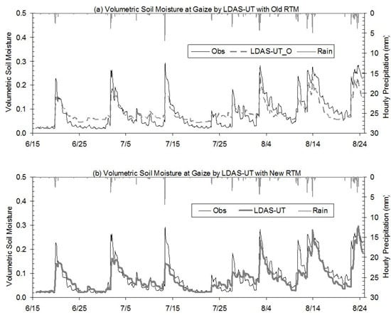
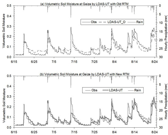
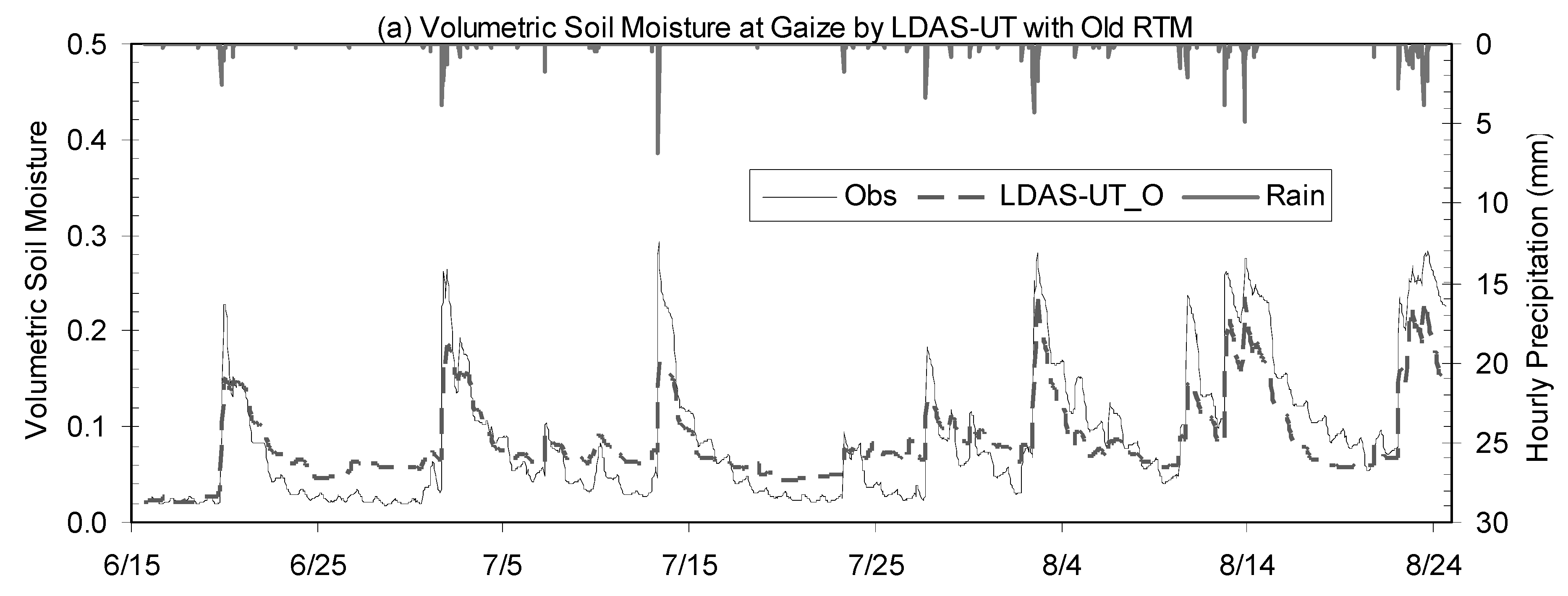
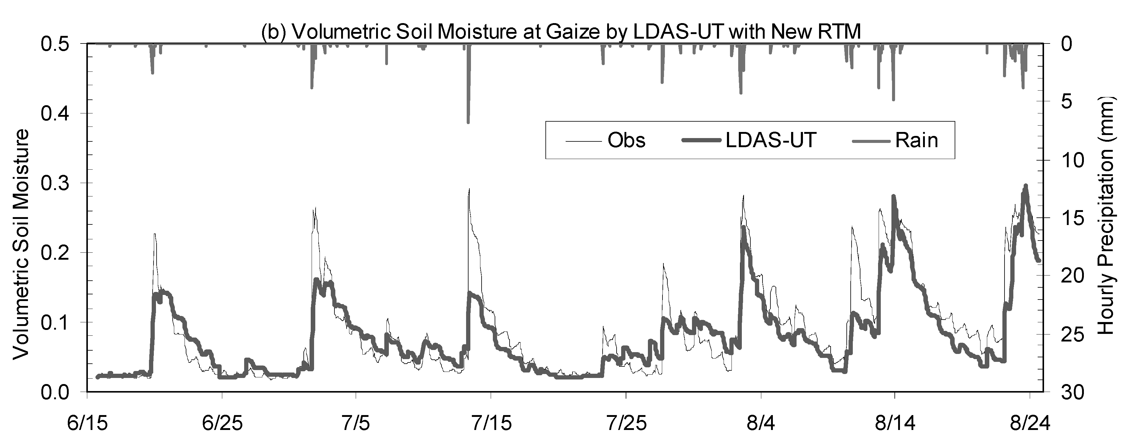
Figure 2 shows the comparison of in-situ observed surface soil mositure with those simulated by LDAS-UT, in which (a) the old RTM is used (named as LDAS-UT_O), and (b) the new RTM is used (named as LDAS-UT_N). The hourly rainfall is also plotted on the upper axis to assist. It is clear that rainfall events mainly occur during August. The accumulated rainfall from 15 June to 31 July is 44.5 mm, while that from 1 August 1 to 24 is 70.4 mm. The observed soil moisture, therefore, is very dry before August, with a mean value of 6.1%. The land surface in August is getting wet, with a mean value of 13.7%. As shown in Figure 2a, LDAS-UT_O estimates are agreeable with the observations during the wet period (August). However, during the dry period (June to July), LDAS-UT_O overestimates soil moisture in general. By contrast, as shown in Figure 2b, LDAS-UT_N produces fairly good estimates of soil moisture, for both wet and dry periods. By comparing the LDAS-UT performance shown in Figure 2a,b, the improvement of soil moisture estimations which result from the new RTM can be confirmed.

Figure 2. Comparison of in-situ observed hourly near surface soil moisture content with those estimated by (a) LDAS-UT with old RTM; and (b) LDAS-UT with new RTM, at Gaize site.

Figure 2. Comparison of in-situ observed hourly near surface soil moisture content with those estimated by (a) LDAS-UT with old RTM; and (b) LDAS-UT with new RTM, at Gaize site.

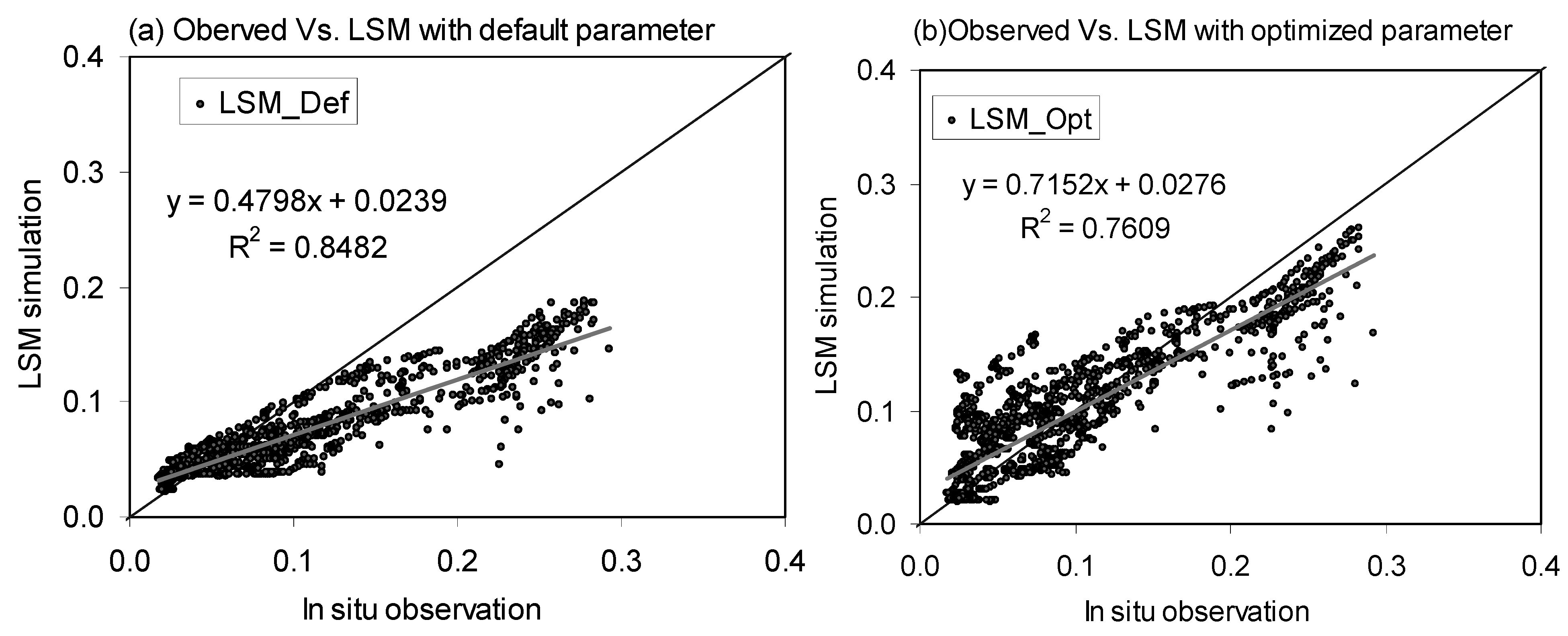
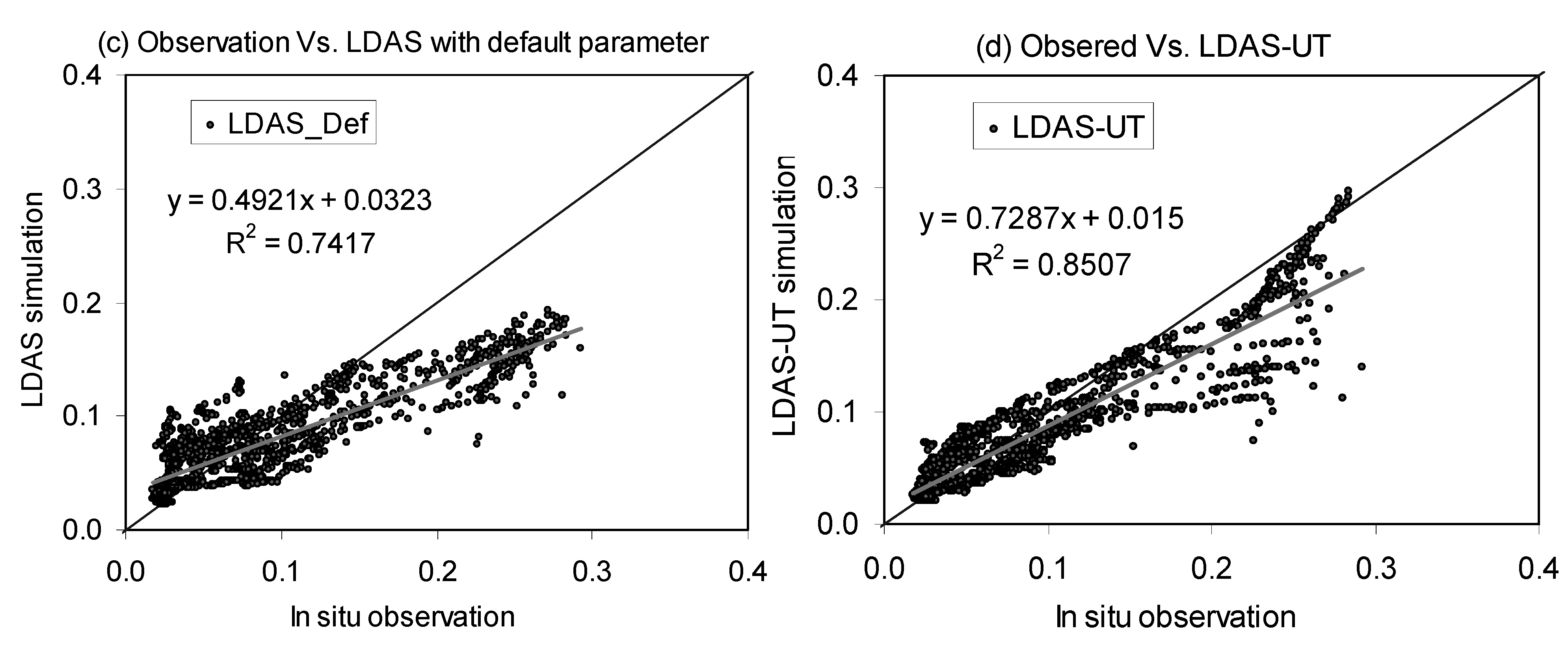
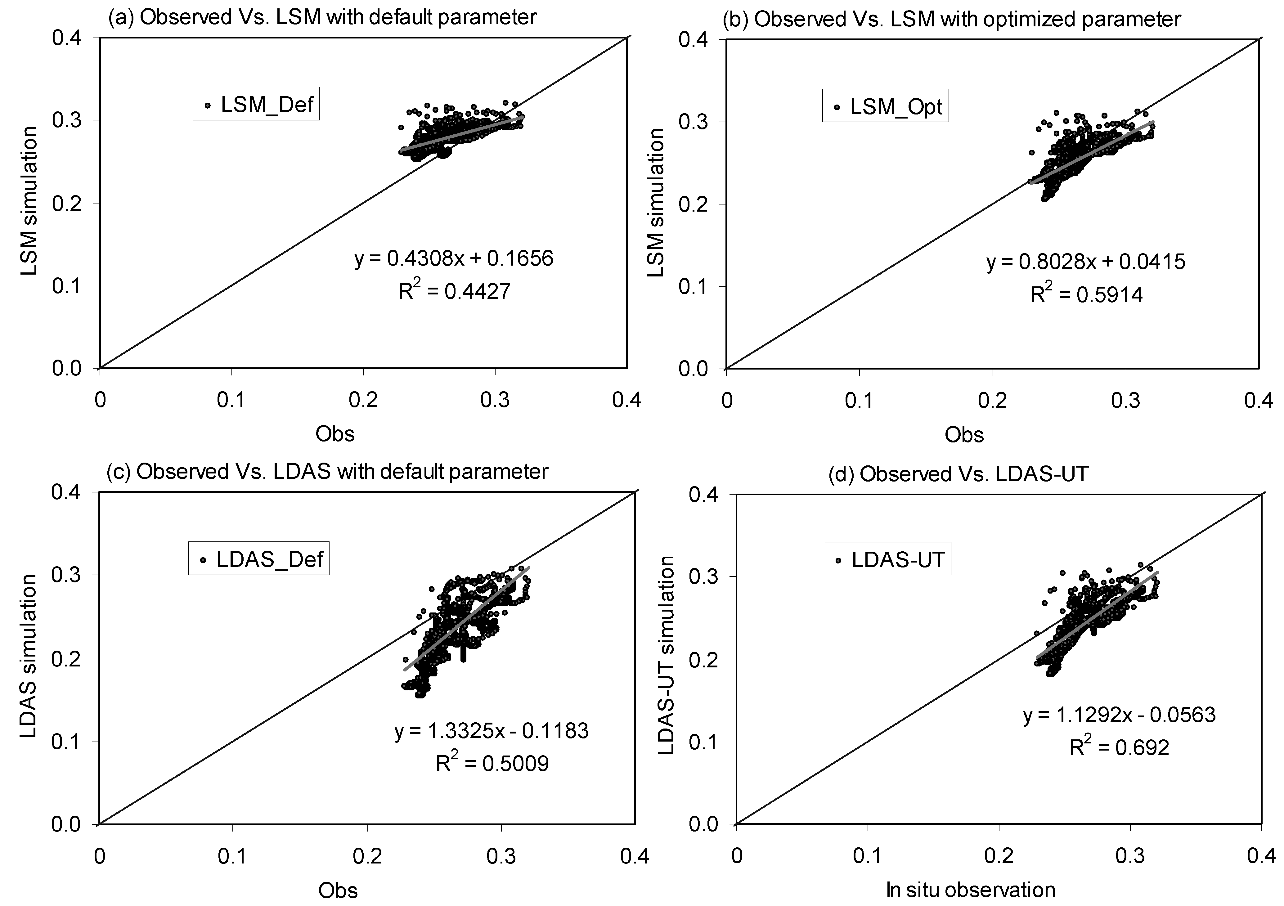
To explain how the parameter optimization pass and data assimilation pass of LDAS-UT contribute to improving soil moisture estimations, the following numerical experiments were designed: (1) LSM only with default parameters, named as LSM_Def; (2) LSM only with LDAS-UT optimized parameters, named as LSM_Opt; (3) data assimilation run with default parameters, named LDAS_Def; and (4) full LDAS-UT run, which means data assimilation run with optimized parameters. Figure 3 shows comparisons between four simulations with in situ observations. An unconstrained linear regression line was also plotted, with slope (BIAS) and intercept (INTER). As we know, the BIAS statistic indicated any systematic bias in the relationship between simulations and observations. For ideal case, BIAS should be 1.0. As indicated by the error metrics shown in Table 2 (RMSE, NSEE and BIAS), LDAS-UT has the best accuracy. For LSM only simulation, LSM_Opt performs better than LSM_Def. For the cases default parameters were used, LDAS_Def performs better than LSM_Def. These comparisons demonstrate that: (1) when same parameters (default or optimized) are used, LDAS produce better results than LSM; (2) for same system (LSM or LDAS), using optimized parameters would result in better estimates; (3) the advantages of LDAS-UT is realized through both the parameter optimization and the data assimilation. Accordingly, we can declare that the LDAS-UT is able to reproduce the temporal variations of soil moisture in this arid and bare soil field.

Figure 3. Comparisons of surface soil moisture between in situ observations and (a) LSM simulation with default parameters; (b) LSM simulation with optimized parameters; (c) data assimilation results with default parameters; and (d) LDAS-UT estimations, at Gaize station.

Figure 3. Comparisons of surface soil moisture between in situ observations and (a) LSM simulation with default parameters; (b) LSM simulation with optimized parameters; (c) data assimilation results with default parameters; and (d) LDAS-UT estimations, at Gaize station.

Table 2. Statistics values in near surface soil moisture content at Gaize station. MBE is mean bias error; RMSE is root mean square error; NSEE is normalized standard error of estimate; R is correlation coefficient; BIAS is the slop of linear regression.

	LSM_Def	LSM_Opt	LDAS_Def	LDAS-UT
MBE	−0.021	0.003	−0.012	−0.008
RMSE	0.044	0.034	0.042	0.029
NSEE	39.6%	30.6%	37.8%	26.5%
R	0.921	0.872	0.861	0.922
BIAS	0.480	0.715	0.492	0.729

Table 2. Statistics values in near surface soil moisture content at Gaize station. MBE is mean bias error; RMSE is root mean square error; NSEE is normalized standard error of estimate; R is correlation coefficient; BIAS is the slop of linear regression.

	LSM_Def	LSM_Opt	LDAS_Def	LDAS-UT
MBE	−0.021	0.003	−0.012	−0.008
RMSE	0.044	0.034	0.042	0.029
NSEE	39.6%	30.6%	37.8%	26.5%
R	0.921	0.872	0.861	0.922
BIAS	0.480	0.715	0.492	0.729

3.2. Application on Wenjiang Station

Wenjiang site was selected for the LDAS-UT validation of humid vegetated area. Simulation ran from 1 January to 31 March 2008. It was the early spring period, during which winter wheat is the main crop and after which the paddy field will be dominative in the region. Due to the lack of in-situ vegetation observation, default morphological parameters of Agriculture/C3 grassland were used in SiB2 and fixed during the whole simulation period.

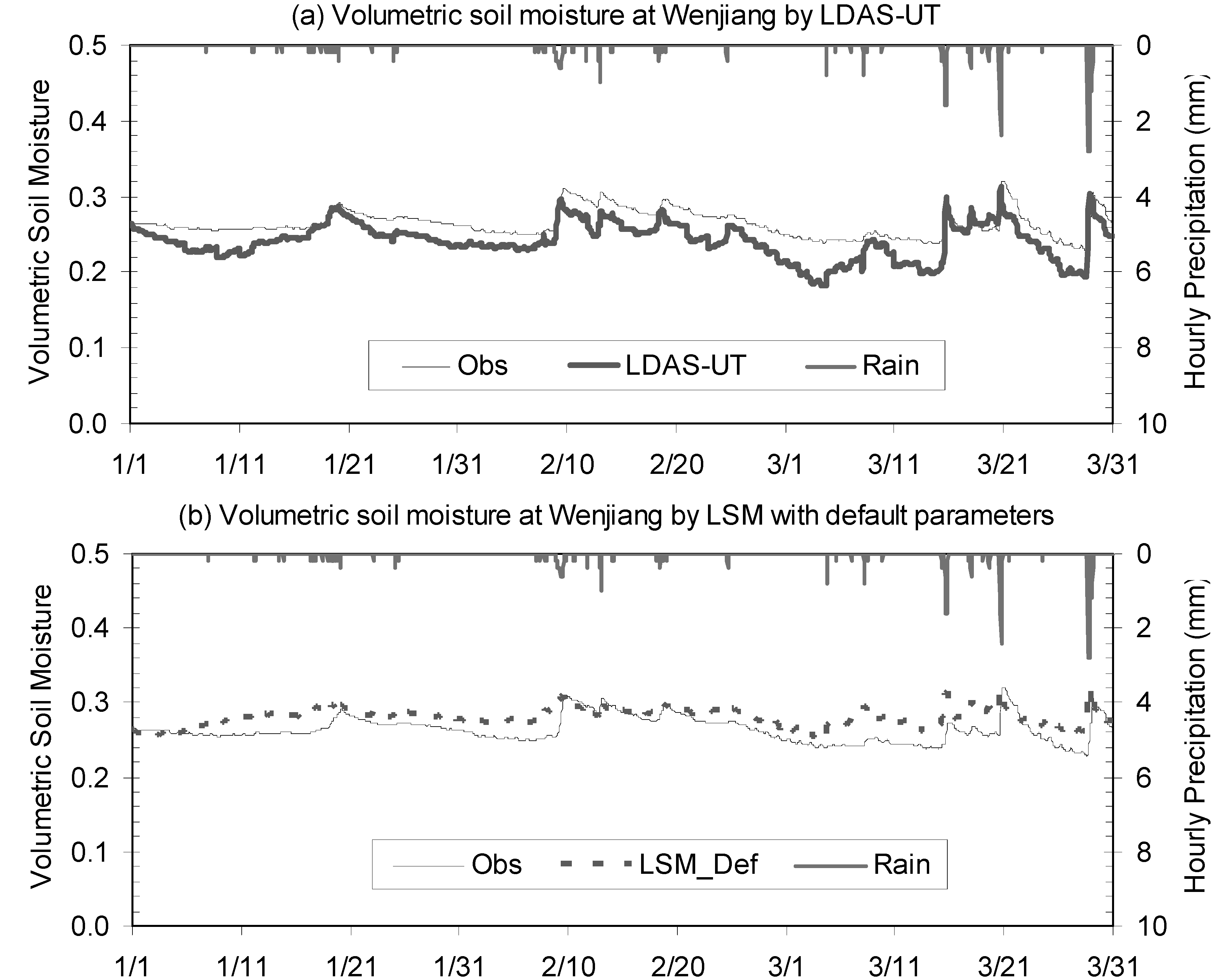
Figure 4a compares the in-situ observed surface soil moisture (by TDR at 4 cm depth) with LDAS-UT output for the whole simulation period. The hourly rainfall is also plotted on the upper axis. LDAS-UT generally predicted the soil moisture peak values in good agreement with the in-situ measurements, for both the occurring time and values. However, the gaps between LDAS-UT estimates and observations are large in the drying processes. The LDAS-UT time series showed that the soil dried out more quickly than the in-situ data did. It is partly due to the fact that the in-situ soil moisture is measured at a depth of 4 cm, which is generally larger than the penetration depth of AMSR-E. The upper shallower soil layer responds more quickly to the atmospheric forcing than the lower deeper layer. In contrast to LDAS-UT performance, as shown in Figure 2b, the LSM generally overestimated soil moisture and even failed to represent clear wet up and dry down processes. One reason for this poor performance is that LSM simulation did not have correct information from remote sensing data. Its errors therefore accumulated, and it even failed to reproduce the temporal variation tendency of surface soil moisture. Another reason for this is the default parameters from the global dataset, which will be discussed in Section 4.3.

Figure 4. Comparison of in-situ observed hourly near surface soil moisture content with (a) LDAS-UT estimation and (b) LSM simulation with default parameters, at Wenjiang station.

Figure 4. Comparison of in-situ observed hourly near surface soil moisture content with (a) LDAS-UT estimation and (b) LSM simulation with default parameters, at Wenjiang station.

Table 3. Statistics values in near surface soil moisture content at Wenjiang station. MBE is mean bias error; RMSE is root mean square error; NSEE is normalized standard error of estimate; R is correlation coefficient; BIAS is the slop of linear regression.

	LSM_Def	LSM_Opt	LDAS_Def	LDAS-UT
MBE	0.016	−0.011	−0.031	−0.022
RMSE	0.020	0.016	0.039	0.026
NSEE	7.6%	6.0%	14.6%	9.8%
R	0.665	0.769	0.708	0.832
BIAS	0.431	0.803	1.333	1.129

Table 3. Statistics values in near surface soil moisture content at Wenjiang station. MBE is mean bias error; RMSE is root mean square error; NSEE is normalized standard error of estimate; R is correlation coefficient; BIAS is the slop of linear regression.

	LSM_Def	LSM_Opt	LDAS_Def	LDAS-UT
MBE	0.016	−0.011	−0.031	−0.022
RMSE	0.020	0.016	0.039	0.026
NSEE	7.6%	6.0%	14.6%	9.8%
R	0.665	0.769	0.708	0.832
BIAS	0.431	0.803	1.333	1.129

Just as done in the Gaize case, four numerical experiments were conducted using Wenjiang forcing data. Figure 5 shows the comparison scatter plots. According to the statistical values shown in Table 3, LDAS-UT simulation has the largest correlation coefficient (R = 0.832), a BIAS (1.129) closest to 1 and a RMSE of 2.6% less than 3% (which is the target accuracy of AMSR-E soil moisture products). These results demonstrate that the LDAS-UT has successfully estimated the surface soil moisture in this humid and vegetated field.

Figure 5. Comparisons of surface soil moisture between in situ observations and (a) LSM simulation with default parameters; (b) LSM simulation with optimized parameters; (c) data assimilation results with default parameters; and (d) LDAS-UT estimations, at Wenjiang station.

Figure 5. Comparisons of surface soil moisture between in situ observations and (a) LSM simulation with default parameters; (b) LSM simulation with optimized parameters; (c) data assimilation results with default parameters; and (d) LDAS-UT estimations, at Wenjiang station.

3.3. Discussion

3.3.1. The Influence of Vegetation Layers

If one only refers to the NSEE values shown in Table 2 for Gaize and Table 3 for Wenjiang, it seems that LDAS-UT performance is better in Wenjiang than in Gaize. However, one should pay attention to the difference in the mean value and variation range for the two data sets. The mean value of Gaize soil moisture series is 8.7%, with a variation range from 1.8% to 29.3%. The mean value of Wenjiang soil moisture series is 26.4%, with a variation range from 22.9% to 32.1%. In order to enable better comparison between two stations, soil moisture time series have been normalized by using the following equation:

$$m^{*}=\frac{m-AVE(m)}{\sqrt{VAR(m)}}$$

(11)

where m is the original soil moisture; AVE(m) represents its average; and VAR(m) represents its variation. After normalization, all soil moisture series have same mean (equal to 0) and variation (equal to 1).

Table 4 show the error metrics of normalized soil moisture simulated by LDAS-UT for Gaize and Wenjiang stations. Both BIAS and NSEE values indicate that LDAS-UT perform better at Gaize than at Wenjiang. This result is expected, since the existence of vegetation at Wenjiang site complicates both the land surface modeling and radiative transfer process modeling. The LAI at Gaize site is very small, around 0.3, which implies that the vegetation effects at Gaize site is negligible.

Table 4. Statistics values in nomorlized soil moisture estimated by LDAS-UT.

	BIAS	NSEE
Gaize	0.922	39.4%
Wenjiang	0.832	58.0%

Table 4. Statistics values in nomorlized soil moisture estimated by LDAS-UT.

	BIAS	NSEE
Gaize	0.922	39.4%
Wenjiang	0.832	58.0%

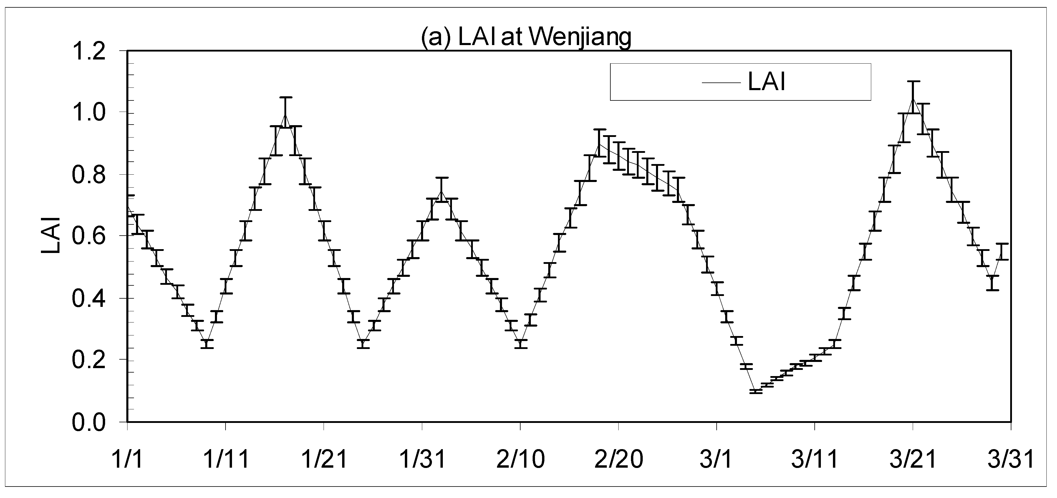
Figure 6a shows the time series of LAI at Wenjiang site, with error bars of ±5%. It is moderately vegetated at Wenjiang in the early spring, giving the maximum LAI of 1.0 (m²/m²) and maximum vegetation water content of 0.4 kg/m² (see Figure 6b, the error bars were derived from 5% LAI errors). By using Equations (3) and (4), transmissivity of vegetation layer can be calculated as:

$$\Gamma =\exp (-{\tau }_c)$$

(11)

Figure 6c shows the transmissivity at 6.9 GHz and 18.7 GHz, with error bars derived from 5% LAI errors. It is clear that the transmissivity at 6.9 GHz is always larger than 0.9, which means that vegetation effects are very small at this frequency. The transmissivity at 18.7 GHz is also larger than 0.7, which means there is some vegetation influence in the brightness temperature but the soil emission is still dominant. From e 6, it is also clear that 5% error of LAI would induce a transmissivity error of around 0.03. The uncertainty of LAI, for this moderate vegetated site, does not produce remarkable errors. These results show that the existence of a moderate vegetation layer does not obstruct microwave remote sensing in detecting the soil moisture variation.

Figure 6. Vegetation information derived from MODIS at Wenjiang: (a) time series of MODIS LAI; (b) derived vegetation water content; (c) calculated transimissivity of vegetation layer at 6.925 GHz and 18.7 GHz.

Figure 6. Vegetation information derived from MODIS at Wenjiang: (a) time series of MODIS LAI; (b) derived vegetation water content; (c) calculated transimissivity of vegetation layer at 6.925 GHz and 18.7 GHz.

At the same time, the existence of a vegetation layer also complicates the modeling of the land surface. As mentioned in Section 4.1, default values were used for vegetation parameters of SiB2. Such arbitrary setting may be inadequate and result in the poor performance of LSM. Fortunately, this problem was partly solved by LDAS-UT, which will be discussed further in the next section. However, for the full solution, dynamic vegetation models and more accurate vegetation information from visible remote sensing and SAR should be addressed.

3.3.2. Parameterization and Data Assimilation

Traditionally, the advantage of a land data assimilation system is to correct the bias of forcing data and/or to overcome the shortage of LSM by merging observation information into the LSM. The superior performance of the LDAS-UT to LSM stems from both data assimilation and parameter optimization.

For the Gaize case, since the quality of forcing data is high (in-situ observed) and the bare soil surface is well modeled, LSM simulates the soil moisture tendency correctly and performs as good as LDAS-UT does (almost same R, shown in Table 2). However, for the absolute values, LSM gives larger MBE, RMSE and NSEE than LDAS-UT. When optimized parameters are used in LSM simulation (LSM_Opt), MBE, NSEE decrease obviously, and BIAS value is almost equal to that of LDAS-UT. The same situation also can be identified by comparing LDAS-UT with LDAS_Def. Therefore, for Gaize station, the improvement is mainly due to the parameter optimization. As shown in Table 5, at the Gaize site, the optimized parameter set has larger porosity than the ISLSCP parameter set, which makes available a higher soil moisture content simulation.

Table 5. Optimized parameters and default parameters at Wenjiang site and Gaize site.

	Wenjiang		Gaize
	Optimized	ISLSCP	Optimized	ISLSCP
Sand (%)	46	34	42	46
Clay (%)	22	31	10	19
Porosity	0.38	0.42	0.35	0.30
b′	0.84	N/A	2.88	N/A
rms height (cm)	0.33	N/A	0.62	N/A
Correlation length (cm)	0.56	N/A	1.88	N/A

Table 5. Optimized parameters and default parameters at Wenjiang site and Gaize site.

	Wenjiang		Gaize
	Optimized	ISLSCP	Optimized	ISLSCP
Sand (%)	46	34	42	46
Clay (%)	22	31	10	19
Porosity	0.38	0.42	0.35	0.30
b′	0.84	N/A	2.88	N/A
rms height (cm)	0.33	N/A	0.62	N/A
Correlation length (cm)	0.56	N/A	1.88	N/A

For the Wenjiang case, due to the existence of a vegetation layer and the usage of default parameters in SiB2, the land surface status was not well simulated. LSM, therefore, failed to represent the soil moisture tendency and showed a poor correlation to ground measurements (R = 0.665). However, LDAS-UT predicted the tendency well (R = 0.832), by correcting the model simulation with remotely sensed information. Moreover, the parameter optimization also contributes to this superior performance of LDAS-UT. As listed in Table 5, at the Wenjiang site, more sandy and less clay soil parameters were generated by LDAS-UT; this parameter set makes soil moisture easier to dry down than the original ISLSCP parameter set.

Besides these advantages obtained by parameter optimization, one should keep in mind that the optimized parameters are dependent on the models and forcing data used in LDAS-UT. They are area-averaged values over AMSR-E footprint, different with in situ observation for both horizontal scales and vertical depth. In this study, due to the lack of in-situ parameters observation, we cannot compare the optimized parameters with in-situ ones. Yang et al. [32] compared the optimized parameters to the observed ones in Mongolia site, and found that optimized soil porosity and soil water potential at saturation were comparable to the in situ observed values. From their study, it is clear that the optimization pass of LDAS-UT at least is able to estimate the parameters which are most sensitive to the soil moisture variation.

3.3.3. The Role of Microwave Remote Sensing Data

Since the AMSR-E data was used in LDAS-UT, when comparing soil moisture estimated by LDAS-UT to ground measurements, one should keep in mind that there may be obvious differences between two sets and that these discrepancies mainly arise from the horizontal and vertical scale differences.

The location of the two sites was selected with careful consideration of representativeness. The simulation results, therefore, generally have good one-to-one correspondence to the in-situ observations. However, the influence of horizontal scale difference still exists; for example, LDAS-UT underestimated the moisture peaks in the simulation of a very dry period at the Gaize site. The influence of vertical scale difference depends on the soil moisture. It therefore affects the comparison more obviously at the Wenjiang site (wetter) than at Gaize site (drier). Through the normalization achieved by Equation (10), all soil moisture time series were normalized to have same mean (equal to 0) and variance (equal to 1), and these influences can be partly removed.

Although the scale difference impedes the application of remote sensing data, the advantages of using AMSR-E data in LDAS-UT are obvious, as: (1) it serves as the calibration references for parameter optimization and (2) it corrects the bias of LSM in the daily assimilation pass. Such advantages will be more important for the land surface simulation over a big region and/or over ungauged (poorly-gauged) regions. For the former case, in situ forcing data were not available or were partly biased. Under this condition, remote sensing data should be able obtain more reasonable results. As one example by Yang et al. [35], AMSR-E data corrected the bias of forcing data, which missed some rainfall events, and improved the soil moisture estimation. For the application in ungauged regions, since there are no in-situ observations, remote sensing data should work as both calibration references and in providing correct information.

4. Conclusions

LDAS is largely expected to provide accurate temporal and spatial continuous land surface variables for promoting research in many fields such as climate change, weather forecasting, and hydrological modeling. In this study, LDAS-UT, updated with an extended RTM, was applied to two sites with different climate and land cover conditions, to check its capability of estimating surface soil moisture at various environments. Soil moisture output from LDAS-UT and the simulations of LSM were compared with in-situ observations, for both absolute values and normalized values. Major findings from this study are as below:

The soil moisture estimates of LDAS-UT are in good agreement with in-situ observations for application at an arid and bare soil field. The new RTM, which include the radiative transfer process in dry soil media, enables LDAS-UT correct soil moisture estimates for very dry cases. In this station, LSM is able to reproduce the soil moisture variation tendency, but it markedly underestimates soil moisture peak.

LDAS-UT also produces good estimates of temporal variations of near surface soil moisture in a humid and vegetated field. Merging the satellite remote sensing information allows LDAS-UT to perform better than LSM, which overestimates soil moisture at this humid and vegetated field.

By summarizing these two findings, the capability of new LDAS-UT to simulate near surface soil moisture at various environments can be validated. With such confidence, it is possible to reliably estimate the land surface status for the whole Tibet Plateau by using this system. Then, the output of LDAS-UT can be used to promote the study of land–atmosphere interactions at the Tibet Plateau.

The superior performance of the LDAS-UT to LSM stems from both data assimilation and parameter optimization. In LDAS-UT, satellite remote sensing data serves as the calibration reference during parameter optimization pass, and provides the correct observation information during the daily assimilation pass. Such advantages of LDAS-UT should be useful for the land surface simulation over large regions and/or at ungauged basins.

Finally, it should be motioned that LDAS-UT successfully estimates soil moisture in a crop land, but it is possible to further improve its performance and application region by introducing (1) vegetation dynamic model, (2) advanced vegetation RTM and (3) more accurate vegetation information (fractional coverage, vegetation geometry, etc.) by combining multi-sensor remote sensing data (visible and infrared remote sensing and radar).