
High-Resolution Precipitation Datasets in South America and West Africa based on Satellite-Derived Rainfall, Enhanced Vegetation Index and Digital Elevation Model

Abstract
:
1. Introduction
2. Materials and Methods
2.1. Materials

| Name | Data Input | Resolution | Start/End Date | Spatial Extent |
|---|---|---|---|---|
| GPCC | Gr. | 0.25° | 1951/2000 | World-Wide |
| TRMM 3B43 | Sat. + Gr. | 0.25° | 1998/present | 50° S–50° N; all long. |
| PERSIANN CDR | Sat. + Gr. | 0.25° | 1983/present | 50° S–50° N; all long. |
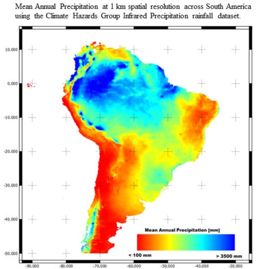
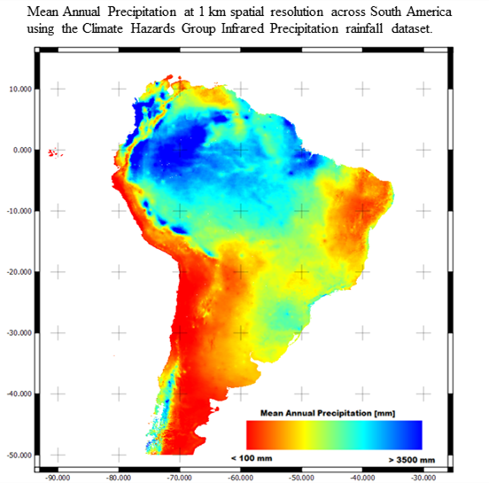
| CHIRP | Sat. + Gr. | 0.05° | 1981/present | 50° S–50° N; all long. |
| CMORPH | Sat. + Gr. | 0.25° | 1998/present | 50° S–50° N; all long. |
| RainFall Estimator | Sat. + Gr. | 0.1° | 2000/present | 40° S–40° N; −20W–55E |
| TAMSAT | Sat. + Gr. | 0.0375° | 1983/2012 | 40° S–40° N; −20W–55E |
2.1.1. GPCC
2.1.2. TRMM 3B43
2.1.3. PERSIANN CDR
2.1.4. CMORPH
2.1.5. CHIRP
2.1.6. RFE
2.1.7. TAMSAT
2.1.8. Vegetation Index: EVI
2.1.9. DEM
2.1.10. Validation Datasets
2.2. Methods
- 1)
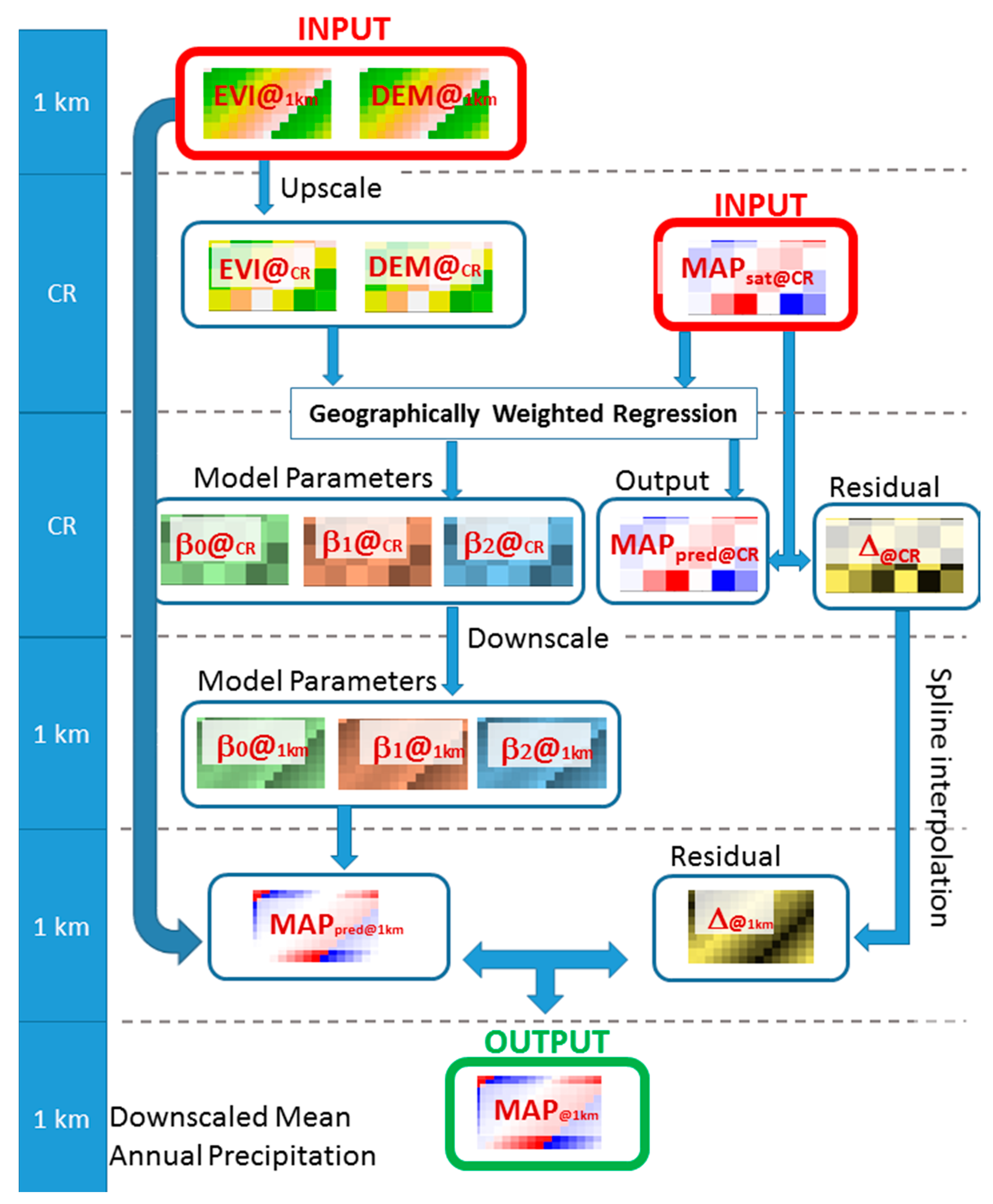
- DEM and average annual EVI are upscaled by pixel averaging from the original fine-scale resolution of 1 km (i.e., DEM@1km and EVI@1km) to the spatial resolution of the satellite-based rainfall dataset (e.g., 25 km for GPCC, 5 km for CHIRP), hereafter DEM@CR and EVI@CR;
- 2)
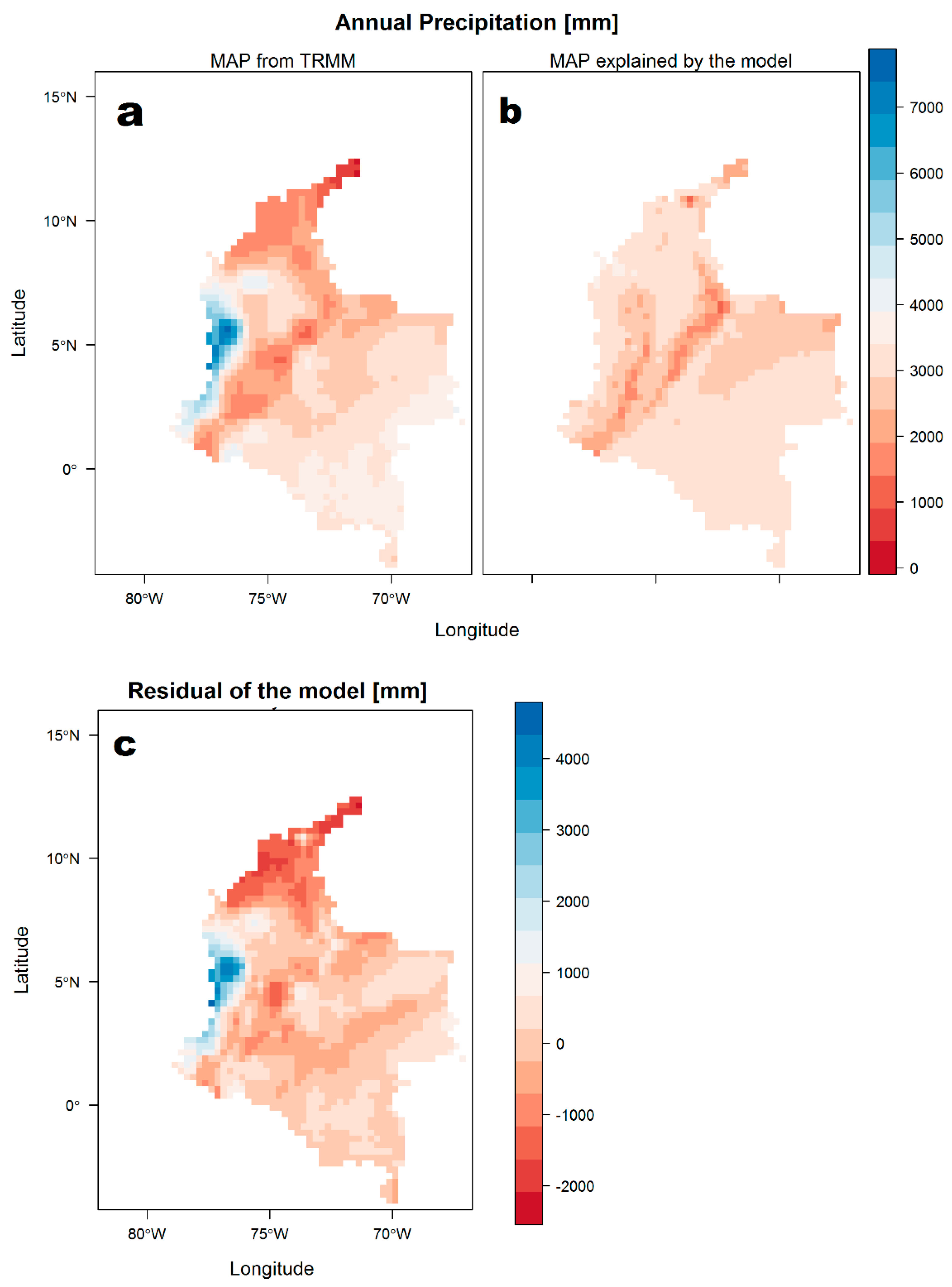
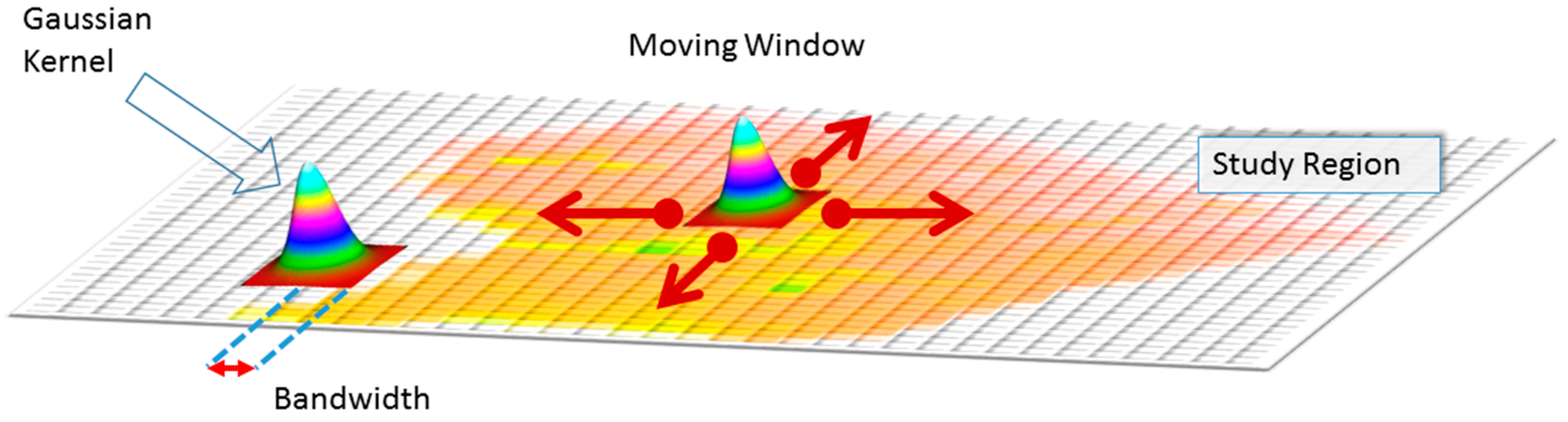
- A Geographically Weighted Regression (GWR, see next subsection for further details) is performed to establish a relationship among MAPsat@CR, DEM@CR and EVI@CR. In essence, the GWR is a local form of linear regression described in the Equation (5):where β0(u), β1(u), and β2(u) are the intercept and the slope parameters, varying with location (u), while ∆@CR is the residual, representing the amount of precipitation that cannot be explained by the model.If we write the regression without the residual component we obtain:where MAPpred@CR is the annual precipitation at coarse resolution predicted/explained using the regression model of DEM and EVI. The closer the value of the predicted rainfall to the satellite-based rainfall, the better the performance of the regression and the lower the value of the residual. The GWR also supplies a per-pixel flag documenting the coefficient of determination of the regression (i.e., r2);
- 3)
- GWR is repeated excluding EVI@CR: in this way we re-compute MAPpred@CR, along with GWR parameters and a map of coefficient of determinations:Step (4) is performed because in some cases there is not a strong relationship between precipitation, DEM and EVI, hence it is beneficial to exclude EVI;
- 4)
- For each cell of the spatial domain, we select the MAPpred@CR , the intercept and slope parameters of the GWR associated with the highest coefficient of determination r2, as shown in Figure 2;
- 5)
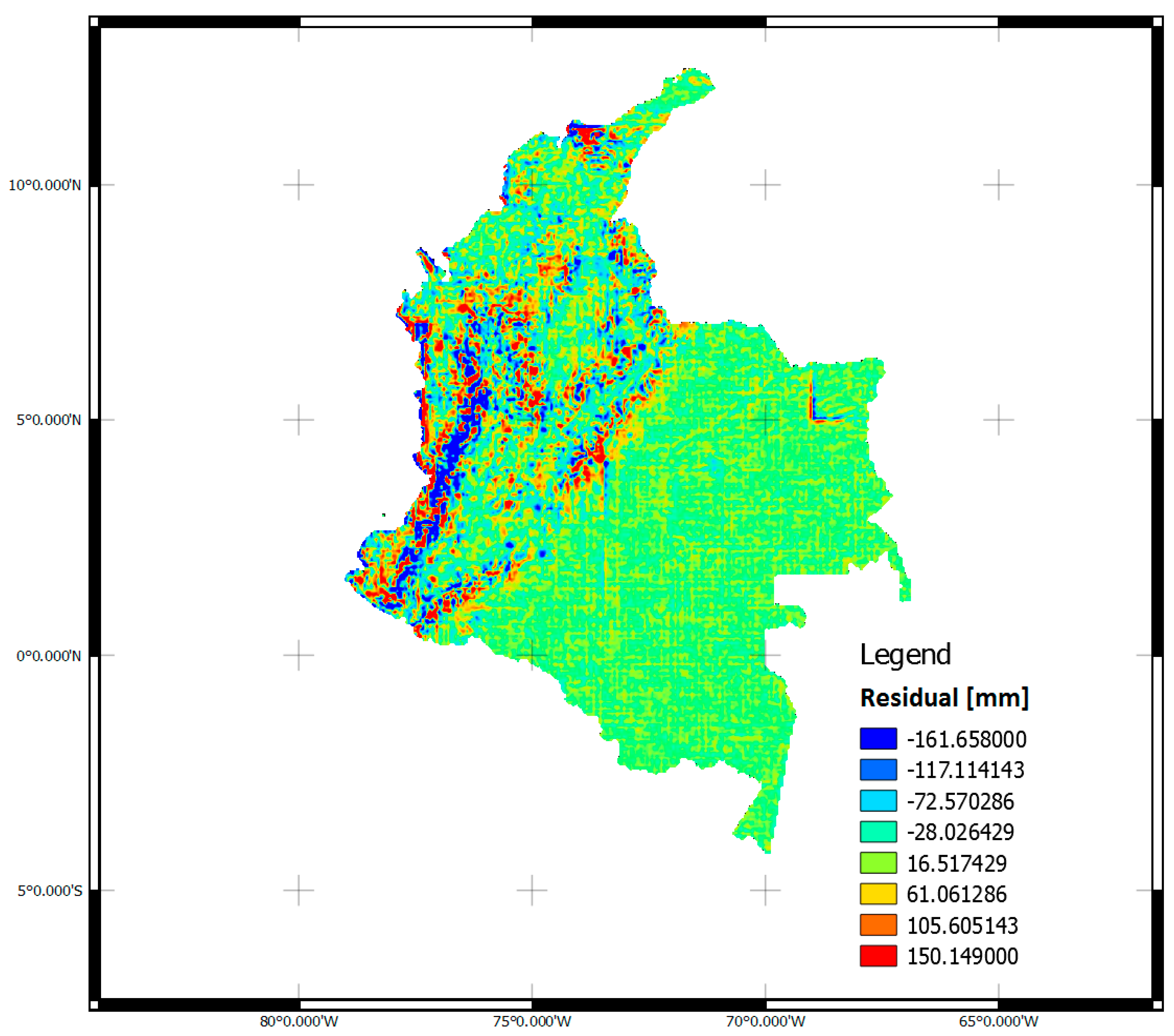
- We subtract MAPpred@CR , obtained in step (5), from MAPsat@CR, obtaining the residual of regression model at coarse resolution, Δ@CR, which represents the amount of precipitation that cannot be explained by the regression based on DEM and EVI;
- 6)
- We downscale Δ@CR to 1 km resolution by applying a cubic spline interpolation, and we obtain Δ@1km;
- 7)
- We downscale the model parameters to 1 km by the nearest neighbour resampling, obtaining thus β0@1km, β1@1km, and β2@1km;
- 8)
- We apply the GWR model with the EVI and DEM at the original spatial resolution of 1 km, obtaining thus the predictive value of annual precipitation with 1 km resolution, hereafter MAPpred@1km:For the cells where EVI values are masked, the corresponding values of the coefficient β2@1km are set equal to zero;
- 9)
- By adding this high resolution predictive precipitation data to the high-resolution residual obtained in step (8), we attain the final downscaled MAP with a 1 km resolution, hereafter MAP@1km, as described below in Equation (9):

Geographically Weighted Regression (GWR)


3. Results
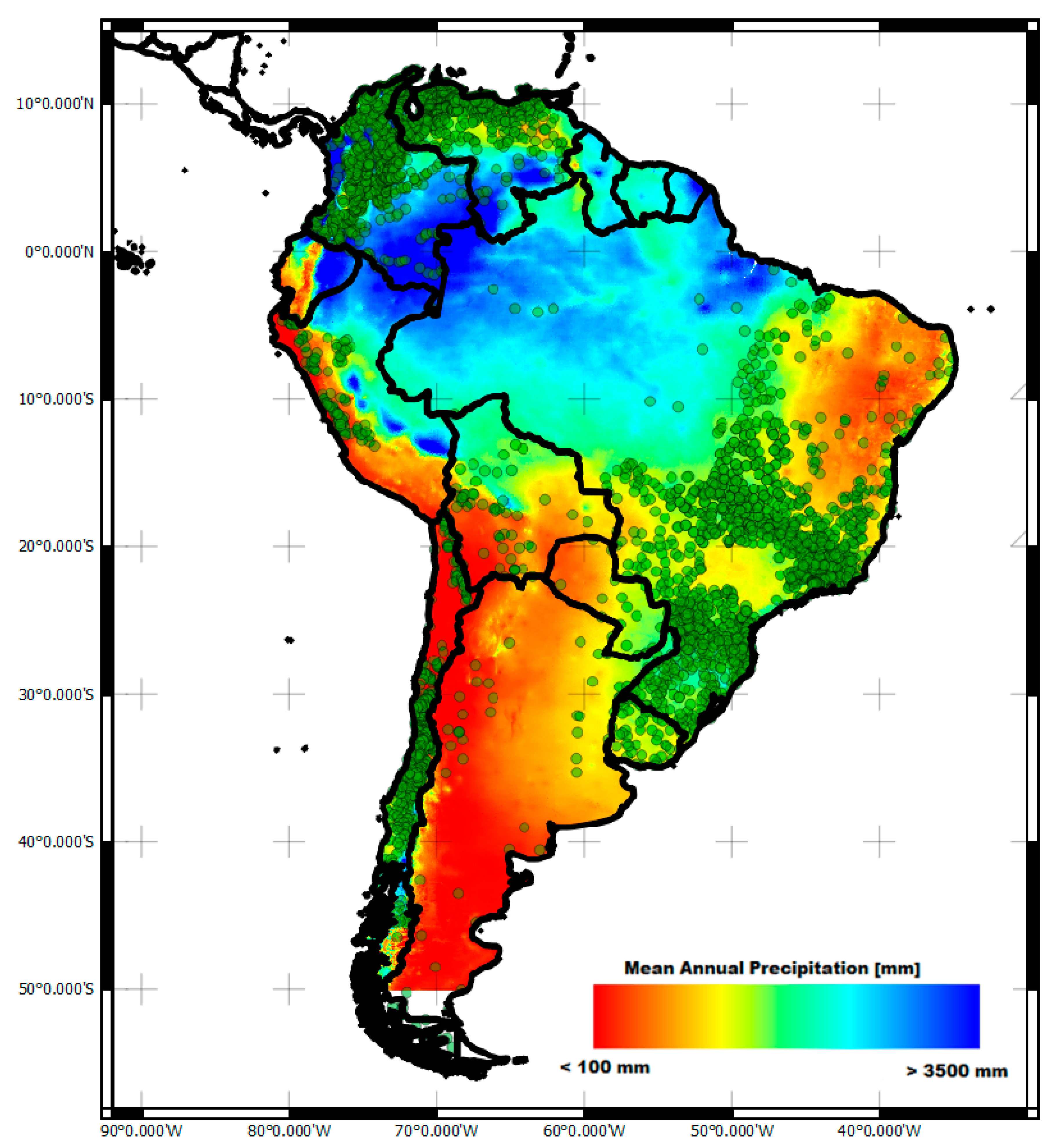
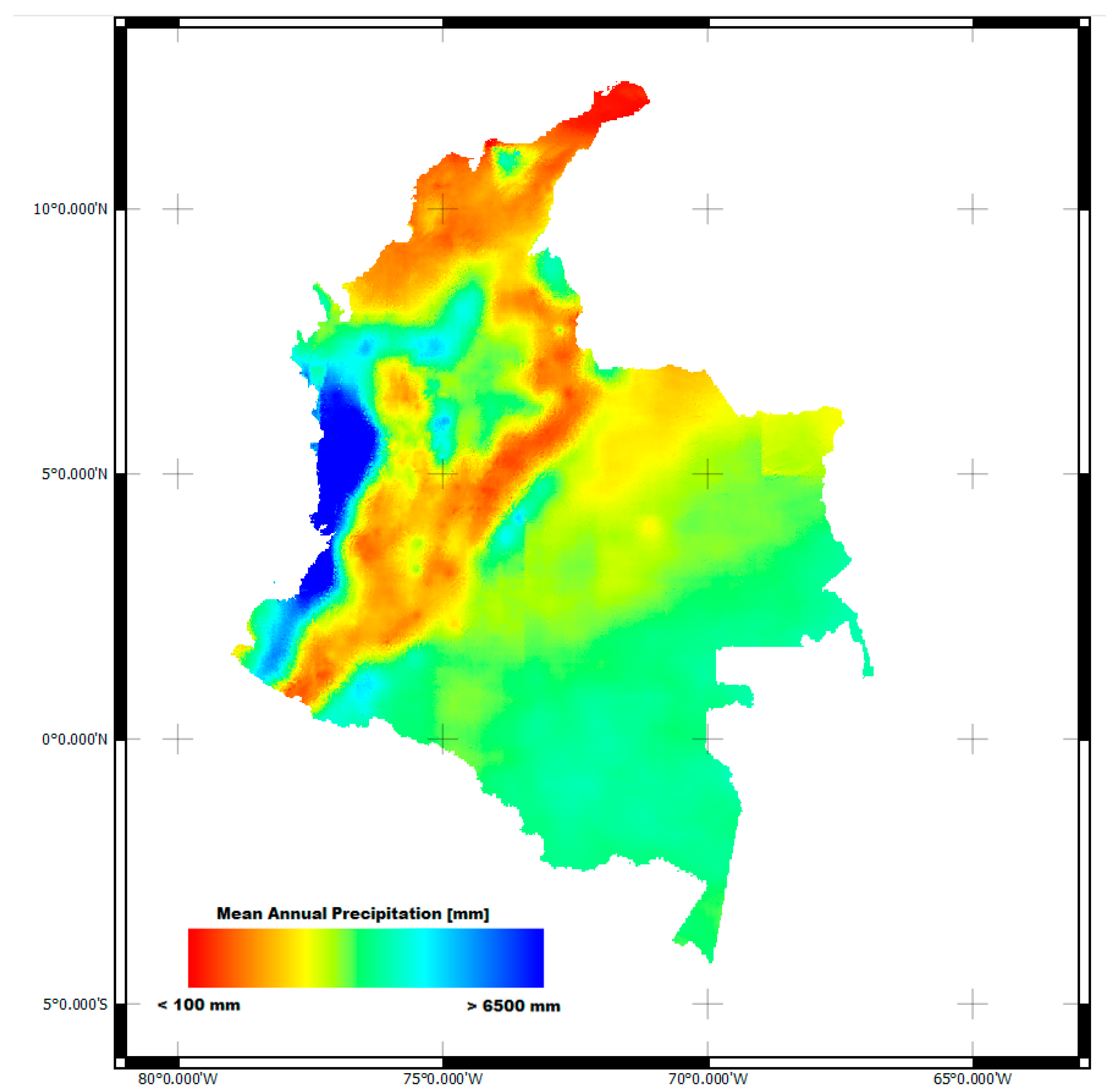
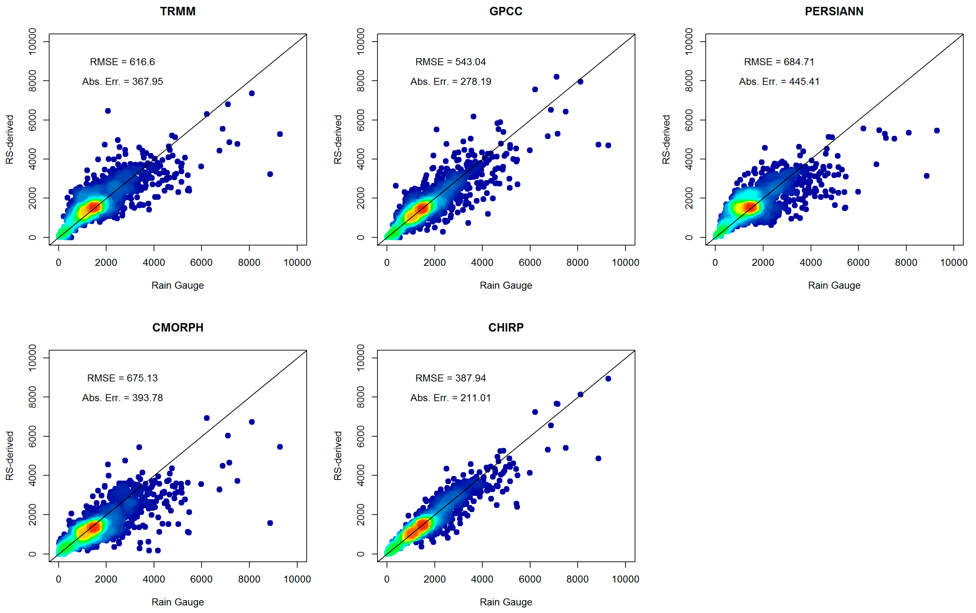
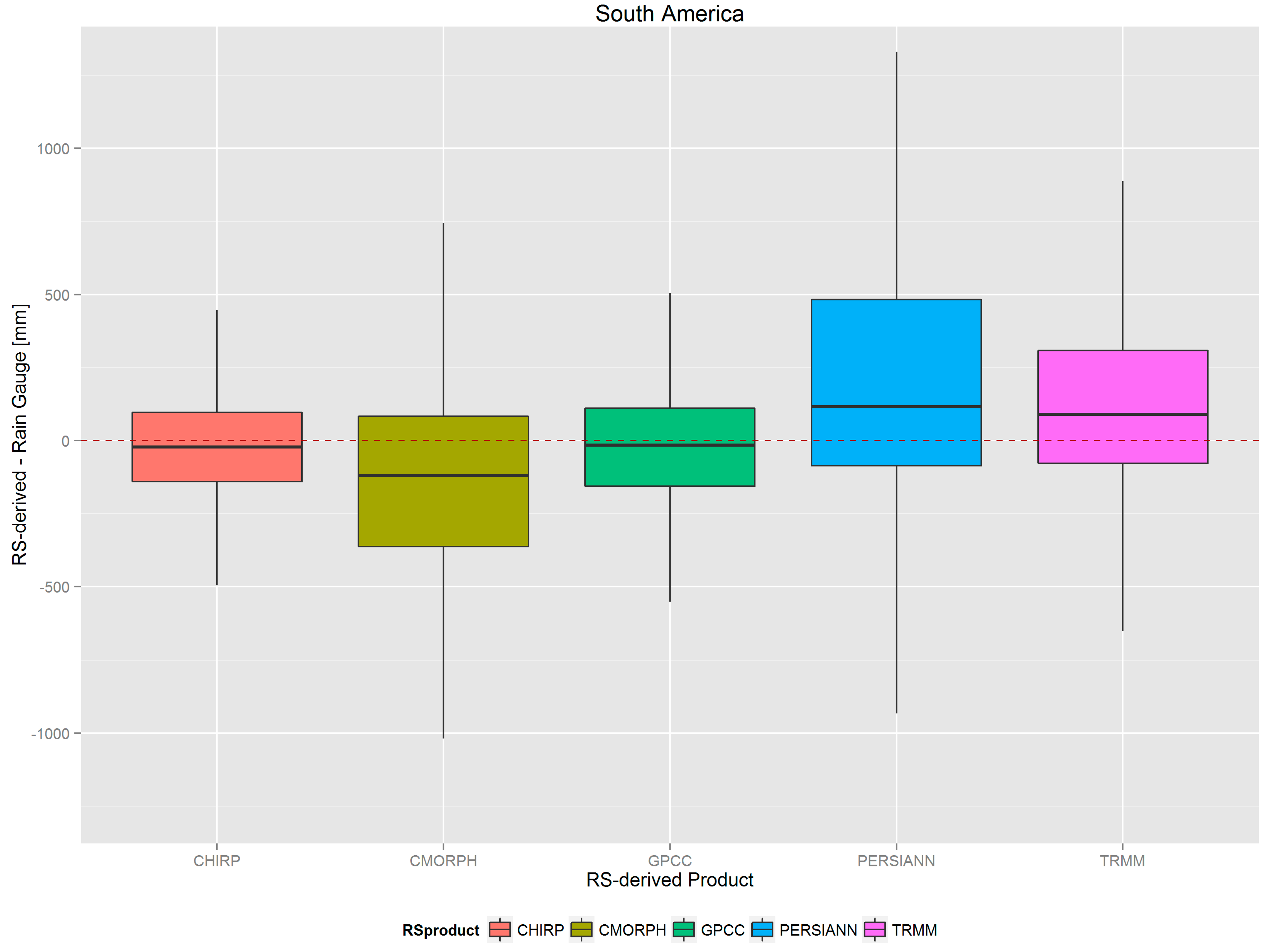
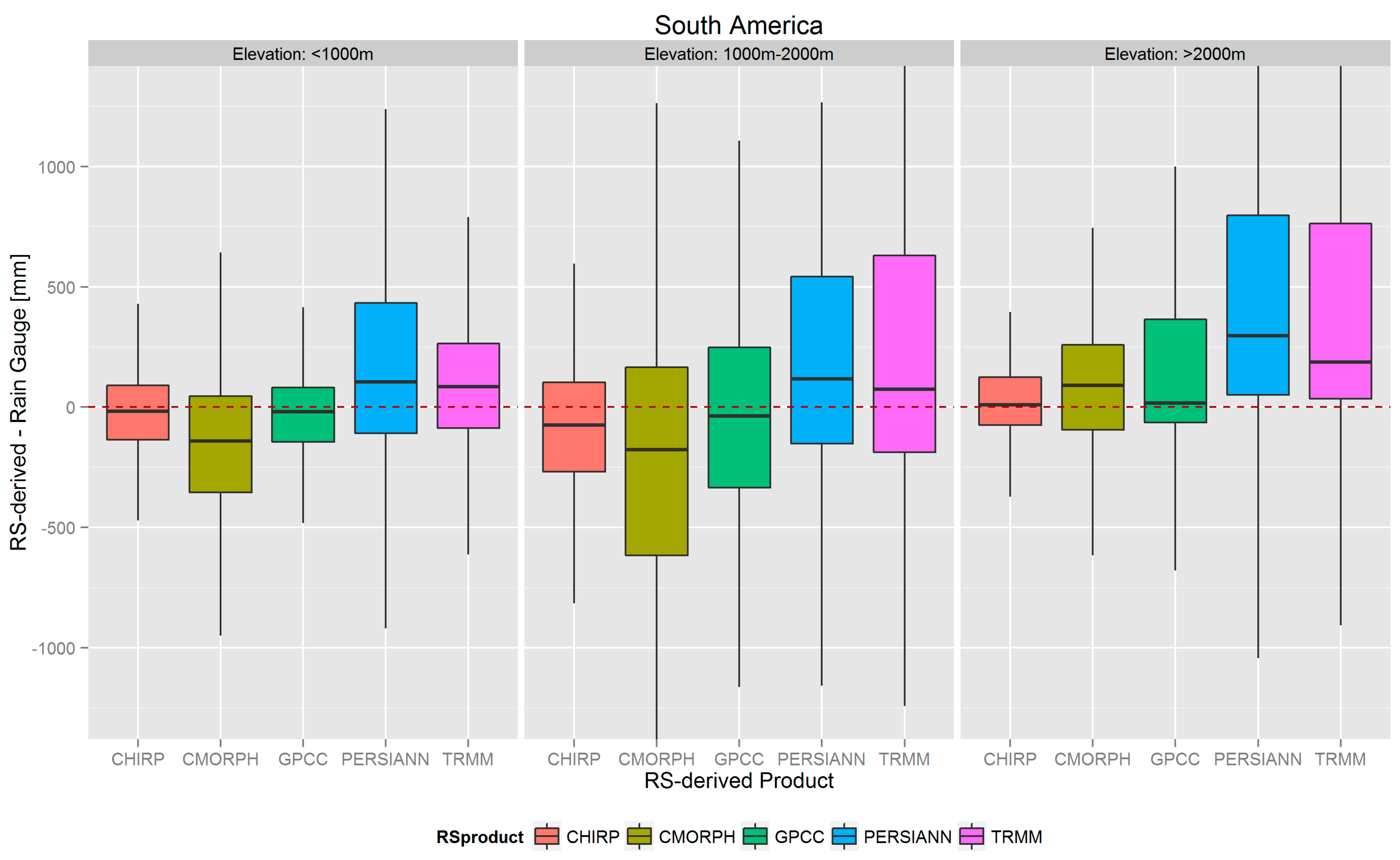
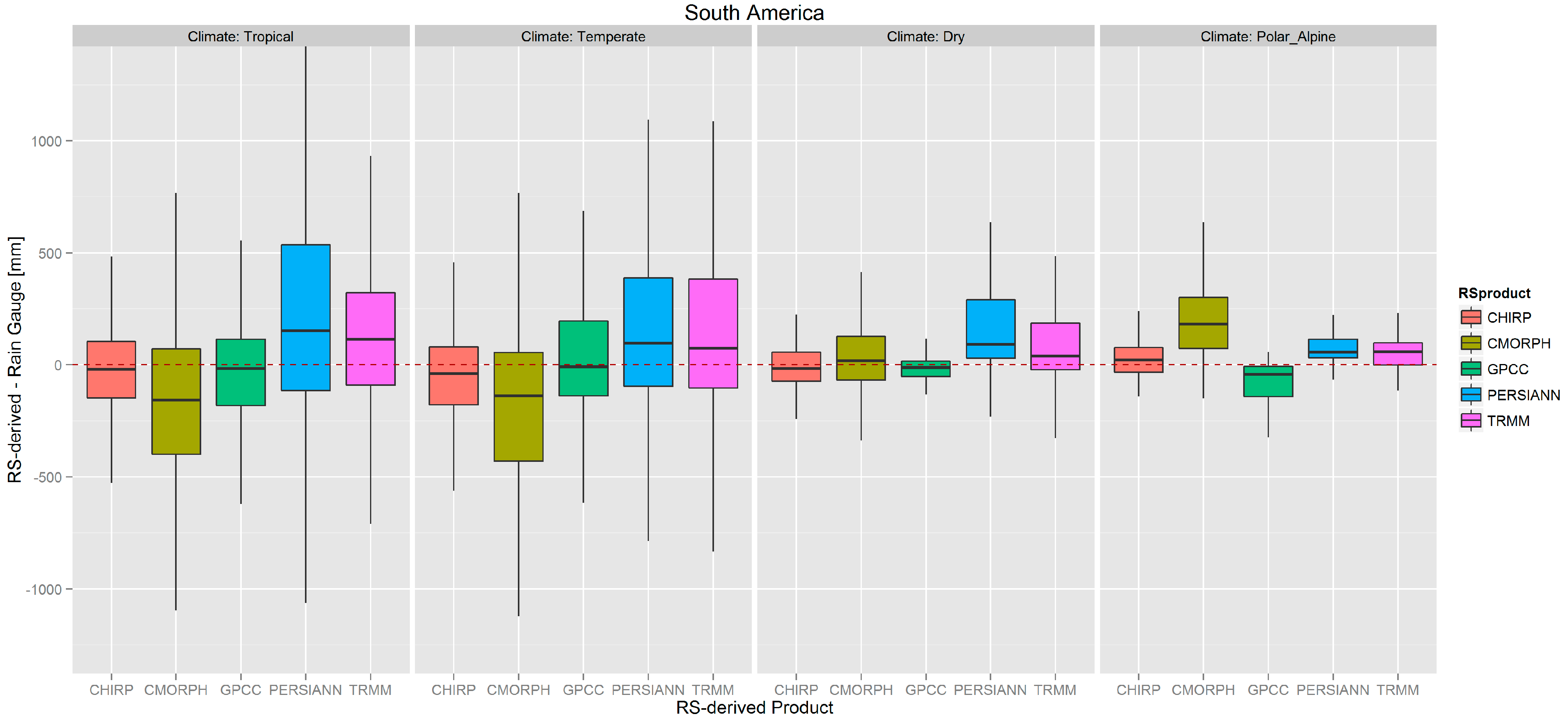
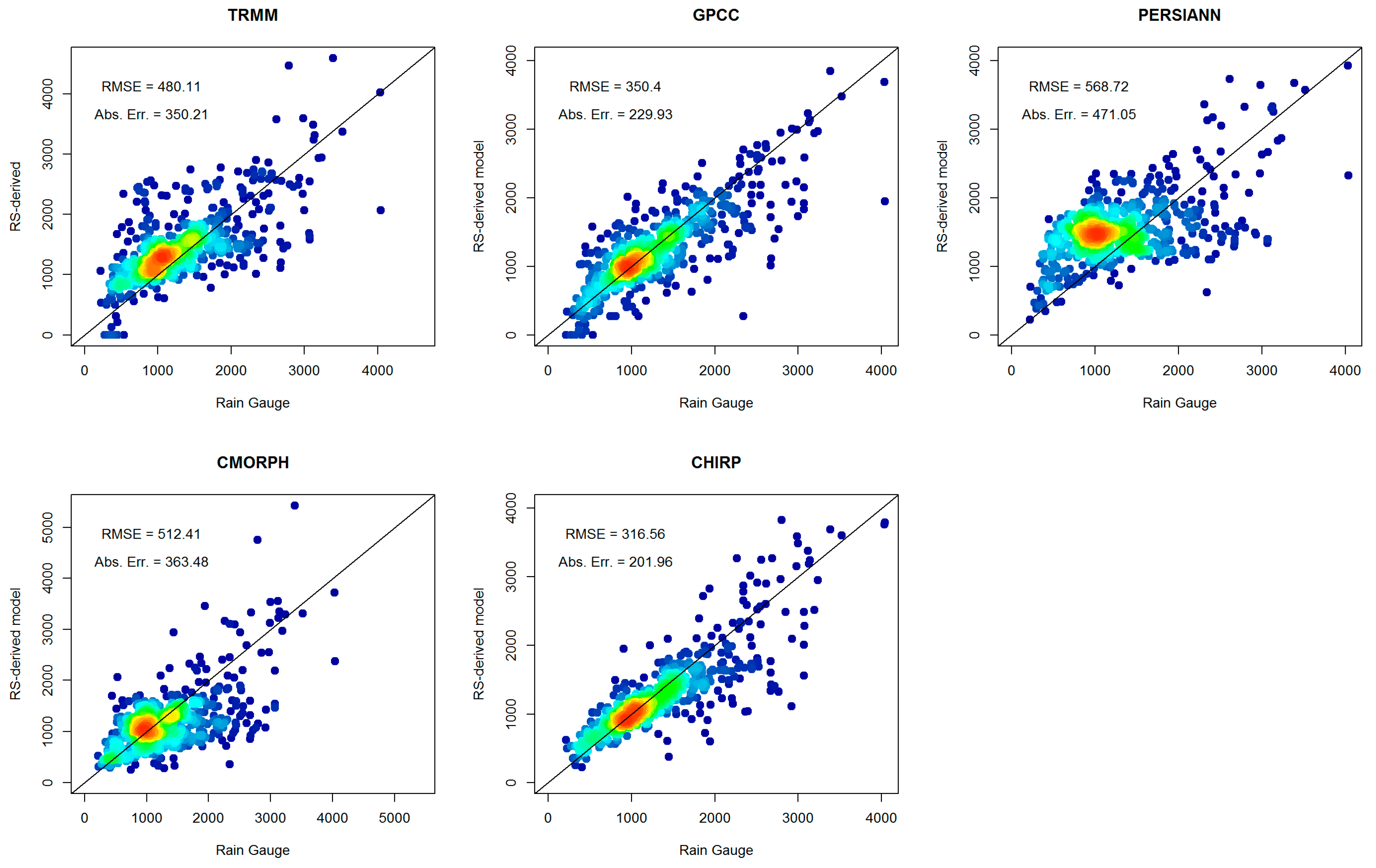
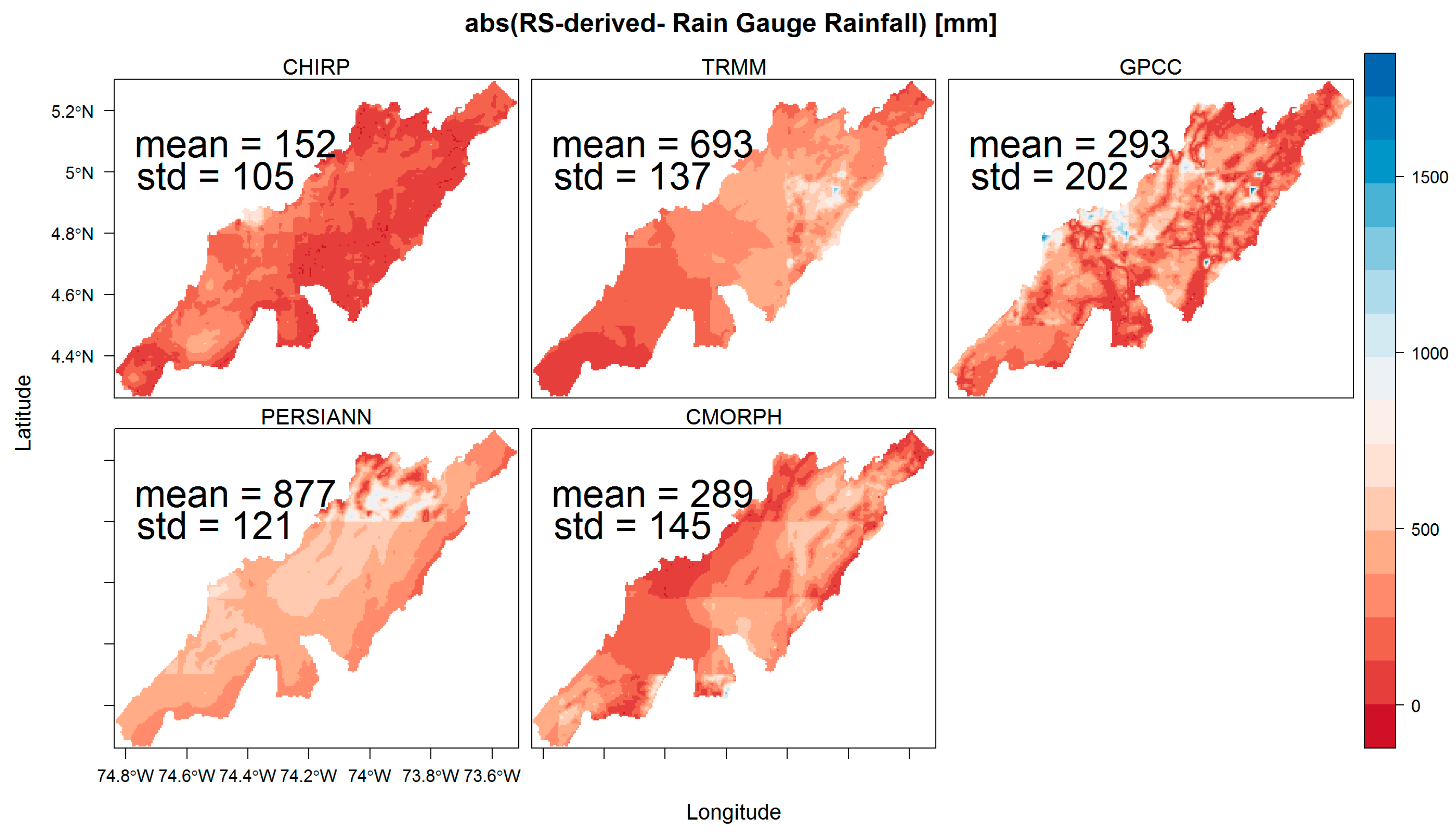
3.1. South America


| Argentina(46) | Bolivia (52) | Brazil (1339) | ||||||||||||
| RMSE | Abs. Err. | MPE | RMSE | Abs. Err. | MPE | RMSE | Abs. Err. | MPE | ||||||
| TRMM | 162.1 | 95.4 | 15.0 | 378.8 | 251.0 | 36.2 | 188.1 | 130.2 | 0.3 | |||||
| GPCC | 104.0 | 54.0 | −1.9 | 219.3 | 149.6 | 13.5 | 145.4 | 103.5 | −0.7 | |||||
| PERSIANN | 255.5 | 168.9 | 44.2 | 505.0 | 347.1 | 45.8 | 221.3 | 155.5 | 0.8 | |||||
| CMORPH | 134.4 | 89.0 | 12.5 | 499.0 | 239.2 | 9.2 | 248.9 | 195.4 | −10.1 | |||||
| CHIRP | 97.7 | 79.2 | −12.9 | 330.7 | 150.9 | −5.0 | 180.9 | 126.4 | −2.2 | |||||
| Chile (344) | Colombia (683) | Paraguay (18) | ||||||||||||
| RMSE | Abs. Err. | MPE | RMSE | Abs. Err. | MPE | RMSE | Abs. Err. | MPE | ||||||
| TRMM | 357.9 | 193.5 | 25.1 | 955.6 | 639.0 | 26.1 | 105.4 | 89.2 | 3.8 | |||||
| GPCC | 381.7 | 197.1 | −4.8 | 871.7 | 502.6 | 5.5 | 60.0 | 44.3 | −0.1 | |||||
| PERSIANN | 523.1 | 284.7 | 30.0 | 1010.6 | 698.0 | 27.6 | 154.9 | 123.6 | 5.8 | |||||
| CMORPH | 466.4 | 318.9 | 66.6 | 1034.7 | 623.4 | −11.2 | 139.8 | 100.1 | −4.3 | |||||
| CHIRP | 279.8 | 160.4 | 13.8 | 570.0 | 311.9 | 1.2 | 86.7 | 67.0 | −5.0 | |||||
| Peru (89) | Uruguay (47) | Venezuela (743) | ||||||||||||
| RMSE | Abs. Err. | MPE | RMSE | Abs. Err. | MPE | RMSE | Abs. Err. | MPE | ||||||
| TRMM | 399.9 | 264.7 | 23.8 | 170.7 | 150.5 | 11.2 | 480.1 | 350.2 | 23.9 | |||||
| GPCC | 354.9 | 244.5 | 16.8 | 103.2 | 75.8 | −4.8 | 350.4 | 229.9 | 1.8 | |||||
| PERSIANN | 440.5 | 353.7 | 72.1 | 166.6 | 146.5 | 11.6 | 568.7 | 471.0 | 37.1 | |||||
| CMORPH | 542.2 | 418.3 | −44.2 | 90.0 | 70.8 | 1.1 | 512.4 | 363.5 | 0.6 | |||||
| CHIRP | 472.8 | 353.2 | −29.7 | 105.1 | 86.4 | 4.3 | 316.6 | 202.0 | 1.1 | |||||

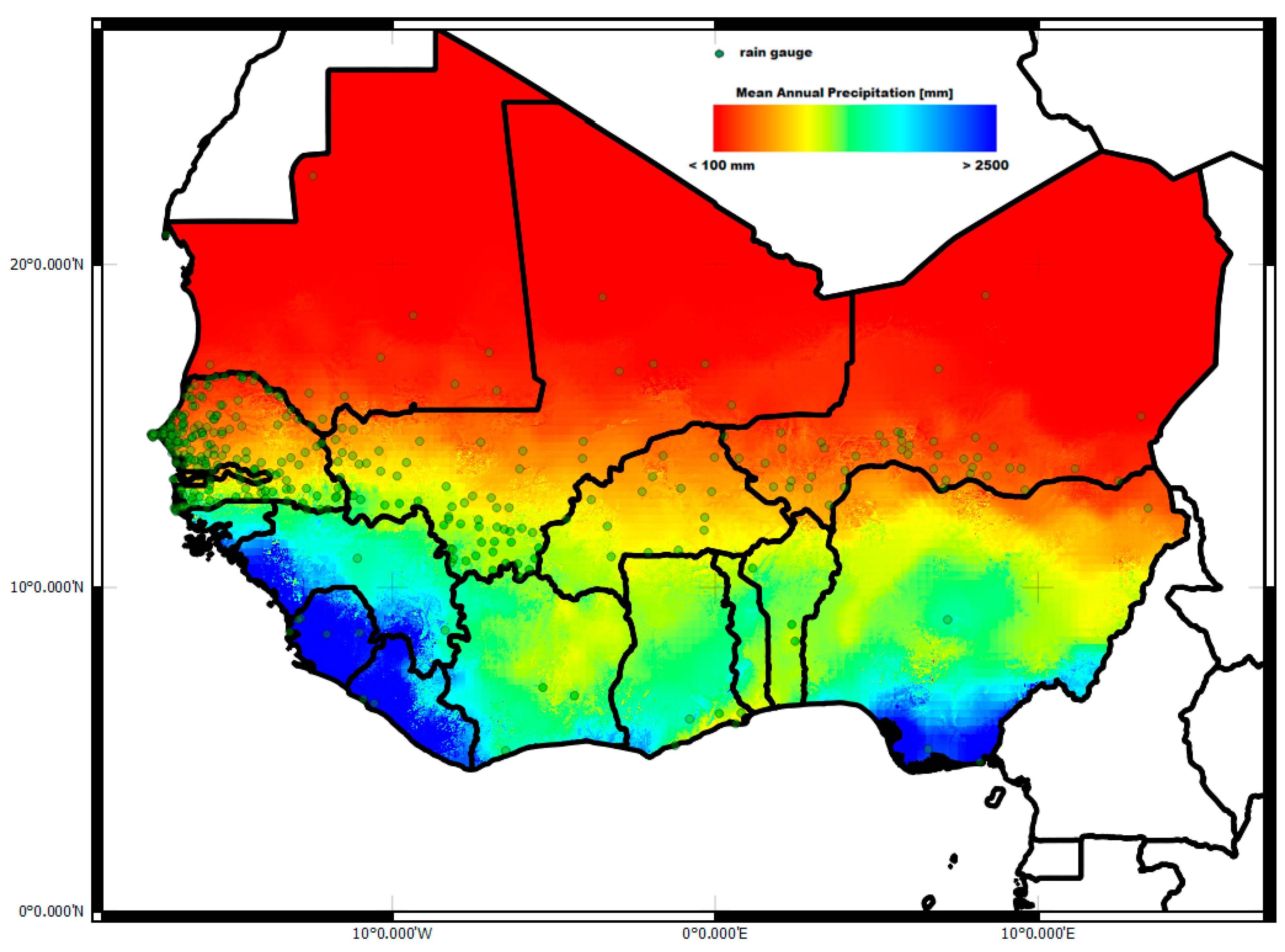
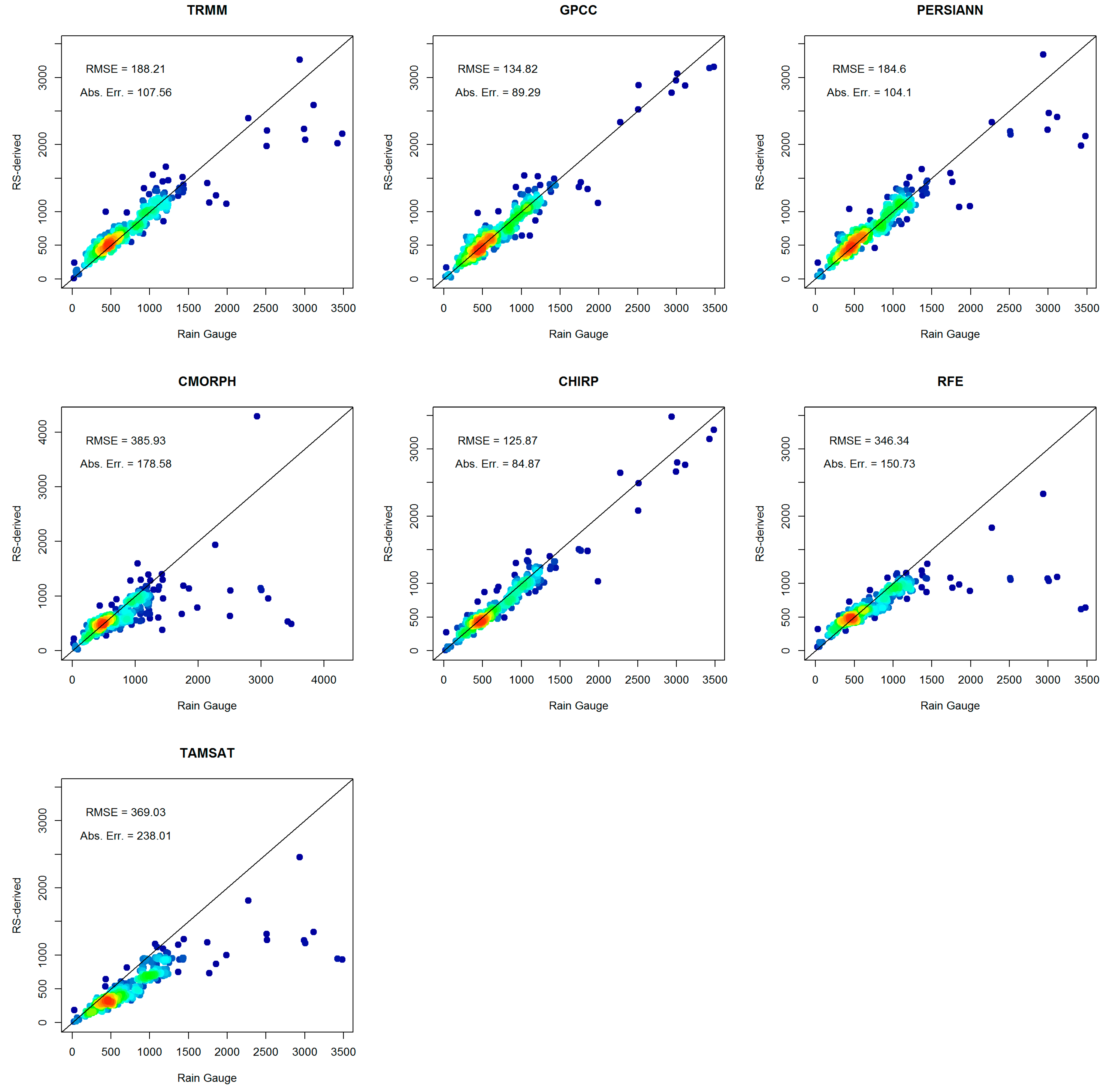
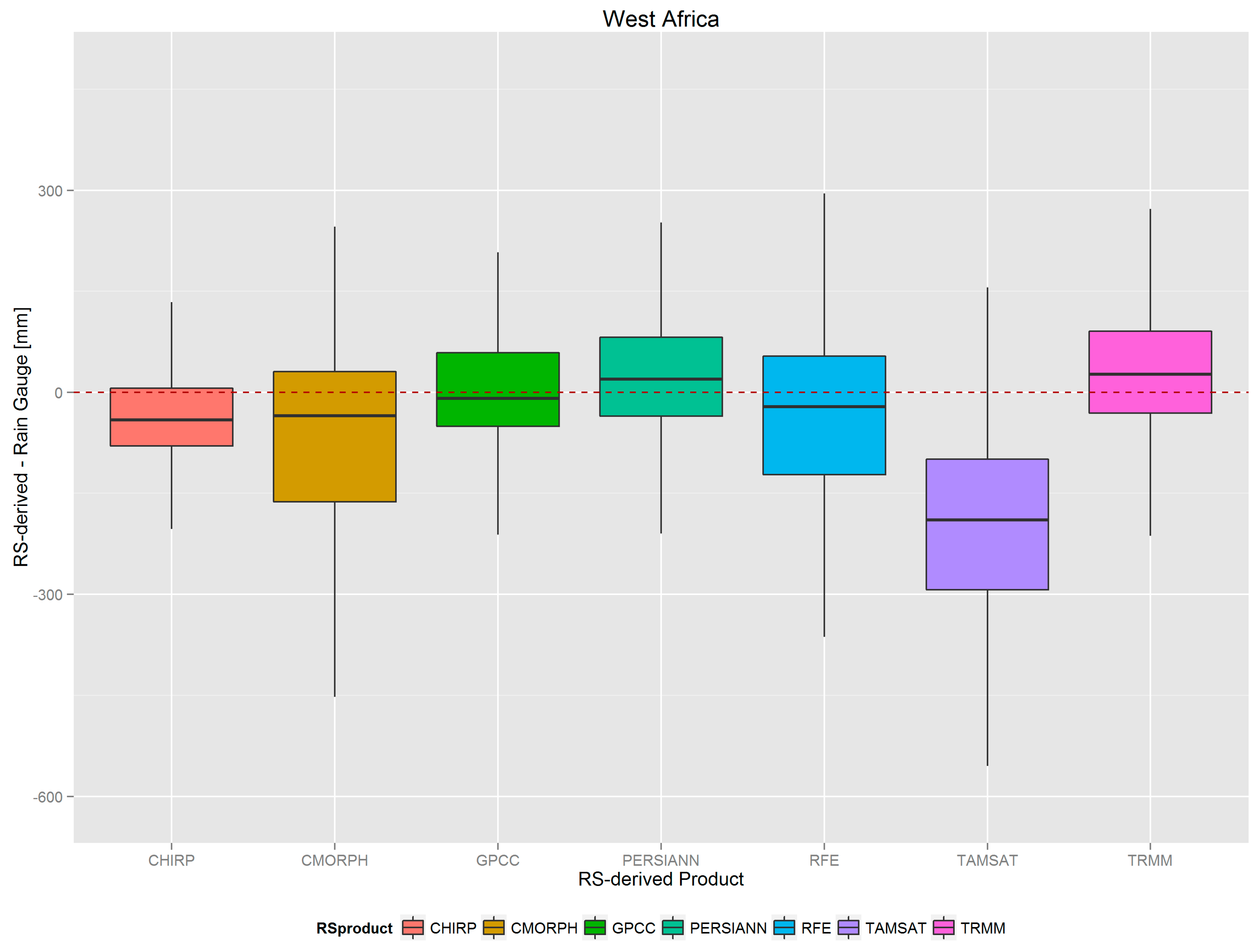
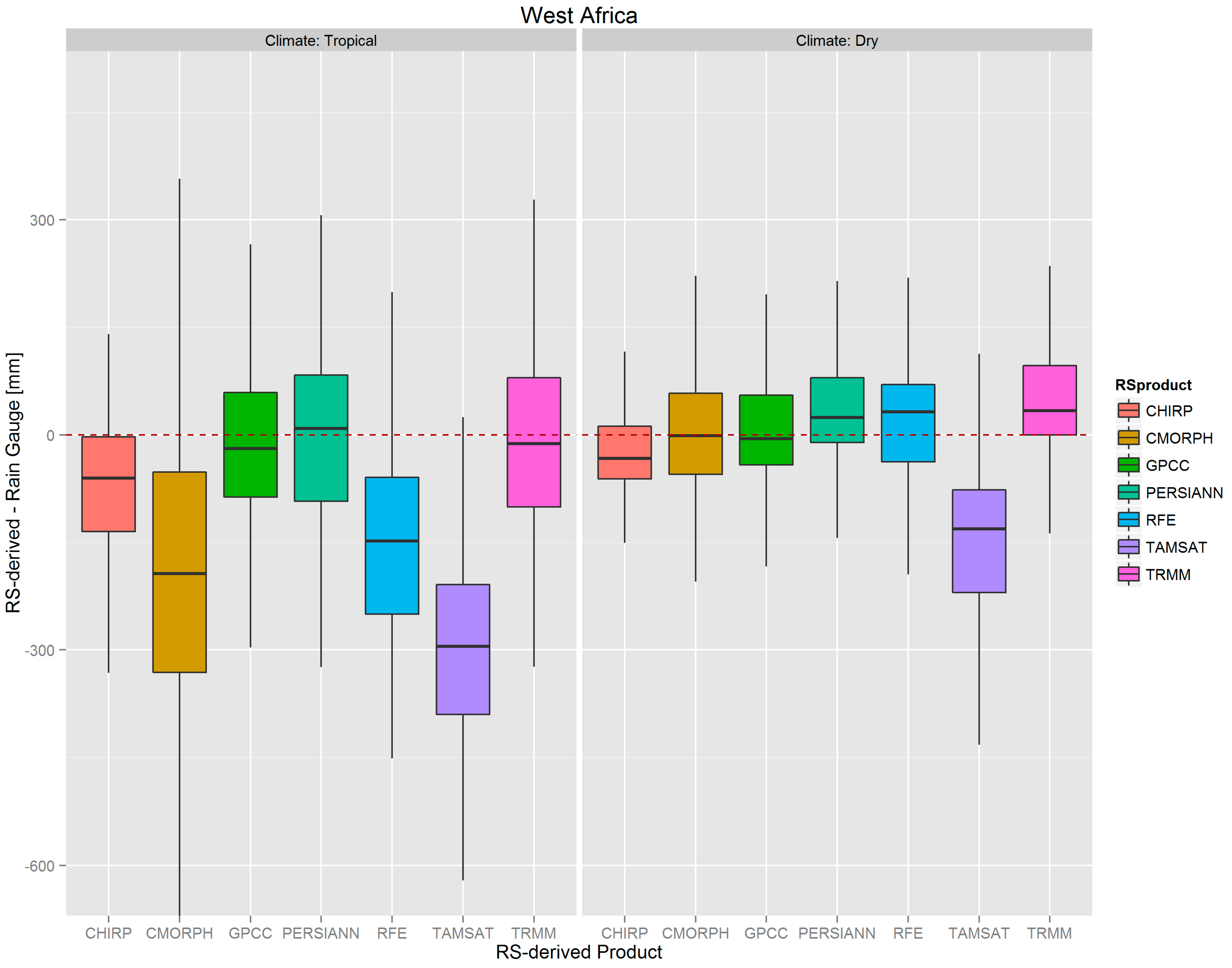
3.2. West Africa


| Burkina Faso (15) | Mali (65) | Mauritania (12) | |||||||
| RMSE | Abs. Err. | MPE | RMSE | Abs. Err. | MPE | RMSE | Abs. Err. | MPE | |
| TRMM | 37.8 | 34.5 | −1.2 | 79.2 | 63.0 | 2.9 | 43.3 | 32.2 | 2.4 |
| GPCC | 51.5 | 40.2 | −5.4 | 83.9 | 58.7 | −3.4 | 30.8 | 23.9 | −4.9 |
| PERSIANN | 42.6 | 35.3 | −1.7 | 82.1 | 63.1 | 1.9 | 27.4 | 21.6 | 2.6 |
| CMORPH | 60.7 | 47.7 | −3.4 | 197.0 | 127.9 | −10.8 | 91.9 | 63.8 | 20.3 |
| CHIRP | 69.6 | 68.1 | −8.8 | 69.0 | 54.3 | −4.7 | 45.8 | 42.0 | −24.7 |
| RFE | 63.2 | 53.9 | 4.5 | 135.7 | 104.0 | −1.8 | 60.9 | 49.0 | 29.2 |
| TAMSAT | 224.8 | 211.5 | −26.4 | 302.5 | 278.8 | −31.8 | 110.2 | 97.6 | −43.1 |
| Niger (44) | Senegal (180) | ||||||||
| RMSE | Abs. Err. | MPE | RMSE | Abs. Err. | MPE | ||||
| TRMM | 42.1 | 33.0 | 11.2 | 165.2 | 118.7 | 20.6 | |||
| GPCC | 43.1 | 34.3 | −4.0 | 158.6 | 113.4 | 12.6 | |||
| PERSIANN | 42.5 | 31.4 | 6.0 | 165.7 | 116.8 | 17.7 | |||
| CMORPH | 63.3 | 47.6 | 3.1 | 200.5 | 139.3 | 3.3 | |||
| CHIRP | 51.4 | 43.4 | −10.1 | 137.2 | 92.7 | 5.6 | |||
| RFE | 68.0 | 59.4 | 18.2 | 166.9 | 111.5 | 5.4 | |||
| TAMSAT | 85.7 | 74.5 | −16.9 | 243.8 | 198.4 | −27.6 | |||
4. Discussion
5. Conclusions
Acknowledgments
Author Contributions
Supplementary Files
Supplementary File 1Conflicts of Interest
References
- Hosking, J.R.M.; Wallis, J.R. Regional Frequency Analysis: An Approach Based on L-Moments; Cambridge University Press: Cambridge, UK, 2005. [Google Scholar]
- Schaefer, M.G. Regional analyses of precipitation annual maxima in Washington State. Water Resour. Res. 1990, 26, 119–131. [Google Scholar] [CrossRef]
- Tapiador, F.J.; Turk, F.J.; Petersen, W.; Hou, A.Y.; García-Ortega, E.; Machado, L.A.T.; Angelis, C.F.; Salio, P.; Kidd, C.; Huffman, G.J.; de Castro, M. Global precipitation measurement: Methods, datasets and applications. Atmos. Res. 2012, 104–105, 70–97. [Google Scholar] [CrossRef]
- Hou, A.Y.; Kakar, R.K.; Neeck, S.; Azarbarzin, A.A.; Kummerow, C.D.; Kojima, M.; Oki, R.; Nakamura, K.; Iguchi, T. The Global Precipitation Measurement Mission. Bull. Am. Meteorol. Soc. 2013, 95, 701–722. [Google Scholar] [CrossRef]
- Guan, H.; Wilson, J.L.; Xie, H. A cluster-optimizing regression-based approach for precipitation spatial downscaling in mountainous terrain. J. Hydrol. 2009, 375, 578–588. [Google Scholar] [CrossRef]
- Rebora, N.; Ferraris, L. The structure of convective rain cells at mid-latitudes. Adv. Geosci. 2006, 7, 31–35. [Google Scholar] [CrossRef]
- Sorooshian, S.; AghaKouchak, A.; Arkin, P.; Eylander, J.; Foufoula-Georgiou, E.; Harmon, R.; Hendrickx, J. M.H.; Imam, B.; Kuligowski, R.; Skahill, B.; Skofronick-Jackson, G. Advancing the remote sensing of precipitation. Bull. Am. Meteorol. Soc. 2011, 92, 1271–1272. [Google Scholar] [CrossRef]
- Huete, A.; Didan, K.; Miura, T.; Rodriguez, E.P.; Gao, X.; Ferreira, L.G. Overview of the radiometric and biophysical performance of the MODIS vegetation indices. Remote Sens. Environ. 2002, 83, 195–213. [Google Scholar] [CrossRef]
- Immerzeel, W.W.; Rutten, M.M.; Droogers, P. Spatial downscaling of TRMM precipitation using vegetative response on the Iberian Peninsula. Remote Sens. Environ. 2009, 113, 362–370. [Google Scholar] [CrossRef]
- Hunink, J.E.; Immerzeel, W.W.; Droogers, P. A High-resolution Precipitation 2-step mapping Procedure (HiP2P): Development and application to a tropical mountainous area. Remote Sens. Environ. 2014, 140, 179–188. [Google Scholar] [CrossRef]
- Jia, S.; Zhu, W.; Lv, A.; Yan, T. A statistical spatial downscaling algorithm of TRMM precipitation based on NDVI and DEM in the Qaidam Basin of China. Remote Sens. Environ. 2011, 115, 3069–3079. [Google Scholar] [CrossRef]
- Park, N.-W. Spatial Downscaling of TRMM precipitation using geostatistics and fine scale environmental variables. Adv. Meteorol. 2013, 2013. [Google Scholar] [CrossRef]
- Fotheringham, A.S.; Brunsdon, C.; Charlton, M. Geographically Weighted Regression: The Analysis of Spatially Varying Relationships, 1st ed.; John Wiley & Sons Inc.: Chichester, England, UK and Hoboken, NJ, USA, 2002. [Google Scholar]
- Foody, G.M. Geographical weighting as a further refinement to regression modelling: An example focused on the NDVI-rainfall relationship. Remote Sens. Environ. 2003, 88, 283–293. [Google Scholar] [CrossRef]
- Chen, F.; Liu, Y.; Liu, Q.; Li, X. Spatial downscaling of TRMM 3B43 precipitation considering spatial heterogeneity. Int. J. Remote Sens. 2014, 35, 3074–3093. [Google Scholar] [CrossRef]
- Brocca, L.; Ciabatta, L.; Massari, C.; Moramarco, T.; Hahn, S.; Hasenauer, S.; Kidd, R.; Dorigo, W.; Wagner, W.; Levizzani, V. Soil as a natural rain gauge: Estimating global rainfall from satellite soil moisture data. J. Geophys. Res.: Atmos. 2014, 119. [Google Scholar] [CrossRef]
- Wood, A.W.; Leung, L.R.; Sridhar, V.; Lettenmaier, D.P. Hydrologic Implications of dynamical and statistical approaches to downscaling climate model outputs. Clim. Chang. 2004, 62, 189–216. [Google Scholar] [CrossRef]
- Becker, A.; Finger, P.; Meyer-Christoffer, A.; Rudolf, B.; Schamm, K.; Schneider, U.; Ziese, M. A description of the global land-surface precipitation data products of the Global Precipitation Climatology Centre with sample applications including centennial (trend) analysis from 1901–present. Earth Syst. Sci. Data 2013, 5, 71–99. [Google Scholar] [CrossRef]
- GPCC. Available online: ftp://ftp.dwd.de/pub/data/gpcc/html/gpcc_normals_v2011_doi_download.html (accessed on 20 August 2014).
- Huffman, G.J.; Bolvin, D.T.; Nelkin, E.J.; Wolff, D.B.; Adler, R.F.; Gu, G.; Hong, Y.; Bowman, K.P.; Stocker, E.F. The TRMM Multisatellite Precipitation Analysis (TMPA): Quasi-global, multiyear, combined-sensor precipitation estimates at fine scales. J. Hydrometeorol. 2007, 8, 38–55. [Google Scholar] [CrossRef]
- TRMM 3B43. Available online: http://trmm.gsfc.nasa.gov/3b43.html (accessed 20 August 2014).
- Ashouri, H.; Hsu, K.-L.; Sorooshian, S.; Braithwaite, D.K.; Knapp, K.R.; Cecil, L.D.; Nelson, B.R.; Prat, O.P. PERSIANN-CDR: Daily precipitation climate data record from multi-satellite observations for hydrological and climate studies. Bull. Am. Meteorol. Soc. 2014, 96. [Google Scholar] [CrossRef]
- PERSIANN CDR. Available online: http://www.ncdc.noaa.gov/cdr/operationalcdrs.html (accessed on 20 August 2014).
- CMORPH. Available online: ftp://ftp.cpc.ncep.noaa.gov/precip/CMORPH_V1.0/ (accessed on 20 August 2014).
- Joyce, R.J.; Janowiak, J.E.; Arkin, P.A.; Xie, P. CMORPH: A method that produces global precipitation estimates from passive microwave and infrared data at high spatial and temporal resolution. J. Hydrometeorol. 2004, 5, 487–503. [Google Scholar] [CrossRef]
- CHIRP. Available online: http://chg.geog.ucsb.edu/data/chirps/ (accessed on 20 August 2014).
- Funk, C.C.; Peterson, P.J.; Landsfeld, M.F.; Pedreros, D.H.; Verdin, J.P.; Rowland, J.D.; Romero, B.E.; Husak, G.J.; Michaelsen, J.C.; Verdin, A.P. A Quasi-Global Precipitation Time Series for Drought Monitoring; U.S. Geological Survey Data Series 832; USGS: Sioux Falls, SD, USA, 2014; p. 4.
- Herman, A.; Kumar, V.B.; Arkin, P.A.; Kousky, J.V. Objectively determined 10-day African rainfall estimates created for famine early warning systems. Int. J. Remote Sens. 1997, 18, 2147–2159. [Google Scholar] [CrossRef]
- Xie, P.; Xiong, A.-Y. A conceptual model for constructing high-resolution gauge-satellite merged precipitation analyses. J. Geophys. Res.: Atmos. 2011, 116. [Google Scholar] [CrossRef]
- RFE. Available online: http://www.cpc.ncep.noaa.gov/products/fews/rfe.shtml/ (accessed on 20 August 2014).
- Maidment, R.I.; Grimes, D.; Allan, R.P.; Tarnavsky, E.; Stringer, M.; Hewison, T.; Roebeling, R.; Black, E. The 30 year TAMSAT African Rainfall Climatology And Time series (TARCAT) data set. J. Geophys. Res.: Atmos. 2014, 119. [Google Scholar] [CrossRef]
- TAMSAT. Available online: http://www.met.reading.ac.uk/~tamsat/data/ (accessed on 20 August 2014).
- Thompson, S.E.; Harman, C.J.; Troch, P.A.; Brooks, P.D.; Sivapalan, M. Spatial scale dependence of ecohydrologically mediated water balance partitioning: A synthesis framework for catchment ecohydrology. Water Resour. Res. 2011, 47. [Google Scholar] [CrossRef]
- Pinty, B.; Verstraete, M.M. GEMI: A non-linear index to monitor global vegetation from satellites. Vegetatio 1992, 101, 15–20. [Google Scholar] [CrossRef]
- Bradley, A.V.; Gerard, F.F.; Barbier, N.; Weedon, G.P.; Anderson, L.O.; Huntingford, C.; Aragão, L.E.O.C.; Zelazowski, P.; Arai, E. Relationships between phenology, radiation and precipitation in the Amazon region. Glob. Change Biol. 2011, 17, 2245–2260. [Google Scholar] [CrossRef]
- Sjöström, M.; Ardö, J.; Arneth, A.; Boulain, N.; Cappelaere, B.; Eklundh, L.; de Grandcourt, A.; Kutsch, W.L.; Merbold, L.; Nouvellon, Y.; et al. Exploring the potential of MODIS EVI for modeling gross primary production across African ecosystems. Remote Sens. Environ. 2011, 115, 1081–1089. [Google Scholar] [CrossRef]
- EVI. Available online: https://lpdaac.usgs.gov/products/modis_products_table/mod13q1 (accessed on 20 August 2014).
- Zhu, Z.; Bi, J.; Pan, Y.; Ganguly, S.; Anav, A.; Xu, L.; Samanta, A.; Piao, S.; Nemani, R.R.; Myneni, R.B. Global data sets of vegetation Leaf Area Index (LAI)3g and Fraction of Photosynthetically Active Radiation (FPAR)3g derived from Global Inventory Modeling and Mapping Studies (GIMMS) Normalized Difference Vegetation Index (NDVI3g) for the period 1981 to 2011. Remote Sens. 2013, 5, 927–948. [Google Scholar] [CrossRef]
- Pekel, J.-F.; Vancutsem, C.; Bastin, L.; Clerici, M.; Vanbogaert, E.; Bartholomé, E.; Defourny, P. A near real-time water surface detection method based on HSV transformation of MODIS multi-spectral time series data. Remote Sens. Environ. 2014, 140, 704–716. [Google Scholar] [CrossRef]
- SWBD. Available online: http://dds.cr.usgs.gov/srtm/version2_1/SWBD/ (accessed on 20 August 2014).
- HydroSHEDS. Available online: http://hydrosheds.cr.usgs.gov/index.php (accessed on 20 August 2014).
- Farr, T.G.; Rosen, P.A.; Caro, E.; Crippen, R.; Duren, R.; Hensley, S.; Kobrick, M.; Paller, M.; Rodriguez, E.; Roth, L.; et al. The shuttle radar topography mission. Rev. Geophys. 2007, 45. [Google Scholar] [CrossRef]
- Lehner, B.; Verdin, K.; Jarvis, A. New global hydrography derived from spaceborne elevation data. Eos. Trans. Am. Geophys. Union 2008, 89, 93–94. [Google Scholar] [CrossRef]
- EUROCLIMA Project. Available online: http://www.euroclima.org/en/euroclima (accessed on 12 December 2014).
- Gollini, I.; Lu, B.; Charlton, M.; Brunsdon, C.; Harris, P. GWmodel: An R Package for Exploring Spatial Heterogeneity Using Geographically Weighted Models. Available online: http://arxiv.org/pdf/1306.0413.pdf (accessed on 17 March 2014).
- Guo, L.; Ma, Z.; Zhang, L. Comparison of bandwidth selection in application of geographically weighted regression: A case study. Can. J. For. Res. 2008, 38, 2526–2534. [Google Scholar] [CrossRef]
- Bowman, A.W. An alternative method of cross-validation for the smoothing of density estimates. Biometrika 1984, 71, 353–360. [Google Scholar] [CrossRef]
- Hurvich, C.M.; Simonoff, J.S.; Tsai, C.-L. Smoothing parameter selection in nonparametric regression using an improved Akaike information criterion. J. R. Stat. Soc. Ser. B Stat. Methodol. 1998, 60, 271–293. [Google Scholar] [CrossRef]
- Hengl, T.; Heuvelink, G.B.M.; Stein, A. A generic framework for spatial prediction of soil variables based on regression-kriging. Geoderma 2004, 120, 75–93. [Google Scholar] [CrossRef]
- Hengl, T.; Heuvelink, G.B.M.; Rossiter, D.G. About regression-kriging: From equations to case studies. Comput. Geosci. 2007, 33, 1301–1315. [Google Scholar] [CrossRef]
- Teng, H.; Shi, Z.; Ma, Z.; Li, Y. Estimating spatially downscaled rainfall by regression kriging using TRMM precipitation and elevation in Zhejiang Province, southeast China. Int. J. Remote Sens. 2014, 35, 7775–7794. [Google Scholar] [CrossRef]
- Meng, Q. Regression kriging versus geographically weighted regression for spatial interpolation. Int. J. Adv. Remote Sens. GIS 2014, 3, 606–615. [Google Scholar]
- Kottek, M.; Grieser, J.; Beck, C.; Rudolf, B.; Rubel, F. World map of the Köppen-Geiger climate classification updated. Meteorol. Z. 2006, 15, 259–263. [Google Scholar] [CrossRef]
- Overeem, A.; Leijnse, H.; Uijlenhoet, R. Country-wide rainfall maps from cellular communication networks. Proc. Natl. Acad. Sci. USA 2013, 110, 2741–2745. [Google Scholar] [CrossRef] [PubMed]
- Qin, Y.; Chen, Z.; Shen, Y.; Zhang, S.; Shi, R. Evaluation of satellite rainfall estimates over the Chinese Mainland. Remote Sens. 2014, 6, 11649–11672. [Google Scholar] [CrossRef]
- Zhang, L.; Potter, N.; Hickel, K.; Zhang, Y.; Shao, Q. Water balance modeling over variable time scales based on the Budyko framework—Model development and testing. J. Hydrol. 2008, 360, 117–131. [Google Scholar] [CrossRef]
- Finley, J.W.; Seiber, J.N. The nexus of food, energy, and water. J. Agric. Food Chem. 2014, 62, 6255–6262. [Google Scholar] [CrossRef] [PubMed]
- Di Baldassarre, G.; Castellarin, A.; Brath, A. Relationships between statistics of rainfall extremes and mean annual precipitation: An application for design-storm estimation in northern central Italy. Hydrol. Earth Syst. Sci. 2006, 10, 589–601. [Google Scholar] [CrossRef]
- AQUAKNOW.NET. Available online: http://www.aquaknow.net/en/home (accessed on 20 August 2014).
© 2015 by the authors; licensee MDPI, Basel, Switzerland. This article is an open access article distributed under the terms and conditions of the Creative Commons Attribution license (http://creativecommons.org/licenses/by/4.0/).
Share and Cite
Ceccherini, G.; Ameztoy, I.; Hernández, C.P.R.; Moreno, C.C. High-Resolution Precipitation Datasets in South America and West Africa based on Satellite-Derived Rainfall, Enhanced Vegetation Index and Digital Elevation Model. Remote Sens. 2015, 7, 6454-6488. https://0-doi-org.brum.beds.ac.uk/10.3390/rs70506454
Ceccherini G, Ameztoy I, Hernández CPR, Moreno CC. High-Resolution Precipitation Datasets in South America and West Africa based on Satellite-Derived Rainfall, Enhanced Vegetation Index and Digital Elevation Model. Remote Sensing. 2015; 7(5):6454-6488. https://0-doi-org.brum.beds.ac.uk/10.3390/rs70506454
Chicago/Turabian StyleCeccherini, Guido, Iban Ameztoy, Claudia Patricia Romero Hernández, and Cesar Carmona Moreno. 2015. "High-Resolution Precipitation Datasets in South America and West Africa based on Satellite-Derived Rainfall, Enhanced Vegetation Index and Digital Elevation Model" Remote Sensing 7, no. 5: 6454-6488. https://0-doi-org.brum.beds.ac.uk/10.3390/rs70506454