
New Spectral Fitting Method for Full-Spectrum Solar-Induced Chlorophyll Fluorescence Retrieval Based on Principal Components Analysis


Abstract
:
1. Introduction
2. Materials and Methods
2.1. Description of Datasets
2.1.1. Simulated Data

| Parameter | Value | Unit | Description | |
|---|---|---|---|---|
| Training | Test | |||
| Cab | 5, 20, 40, 60, 80 | 10, 30, 50, 70 | μg/cm2 | Leaf chlorophyll a + b content |
| Cdm | 2, 10, 20 | 5, 15 | mg/cm2 | Dry matter content |
| Cw | 5, 10, 20, 40 | 10, 30 | 10–3 cm | Leaf water equivalent layer |
| Cs | 0 | 0 | fraction | Senescent material fraction |
| N | 1, 2 | 1.5, 2.5 | - | Leaf thickness parameters |
| LAI | 1, 2, 4, 6 | 1, 3, 5, 7 | m2 /m2 | Leaf area index |
| LIDFa | −0.35 | −0.35 | - | Leaf inclination |
| LIDFb | −0.15 | −0.15 | - | Variation in leaf inclination |
| FQE | 0.04 | 0.02, 0.04 | - | Fluorescence quantum yield efficiency |
| SZA | 20, 60 | 30, 40, 50 | degree | Solar zenith angle |
| VZA | 0, 30, 60 | 0, 20, 40 | degree | View zenith angle |
| RAA | 90 | 90 | degree | Relative azimuth angle |
2.1.2. Field-Measured Data
2.2. SIF Spectra Retrieval
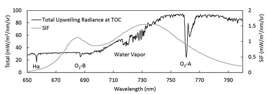
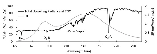
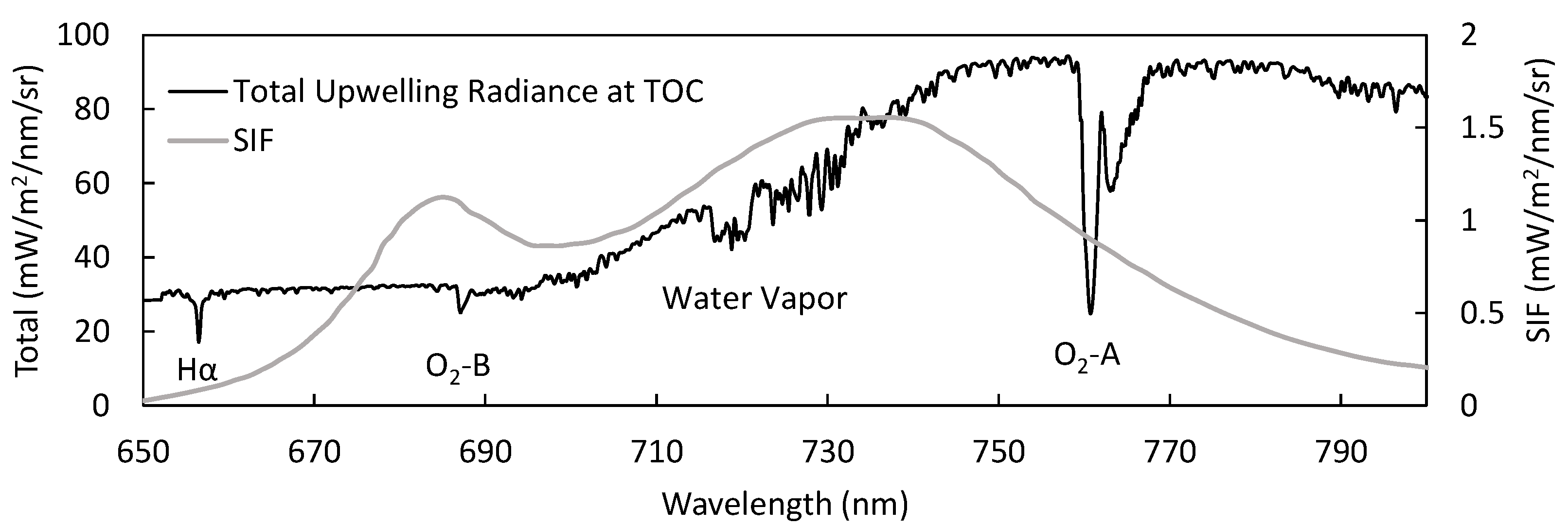
2.2.1. Band Selection

2.2.2. Reconstruction of Reflectance and SIF Spectra


2.2.3. Spectral Fitting
- (1)
- Calculate the apparent reflectance () using the total upwelling radiance and downwelling irradiance.
- (2)
- Estimate the weights of the reflectance PCs using the apparent reflectance () without absorption bands according to Equation (8) and then reconstruct the reflectance using the weights of the different reflectance PCs according to Equation (6).
- (3)
- Estimate the weights of the SIF PCs according to Equation (10) using the least-squares fitting method for the parts of the spectrum within the absorption bands and reconstruct the SIF spectrum according to Equation (7).
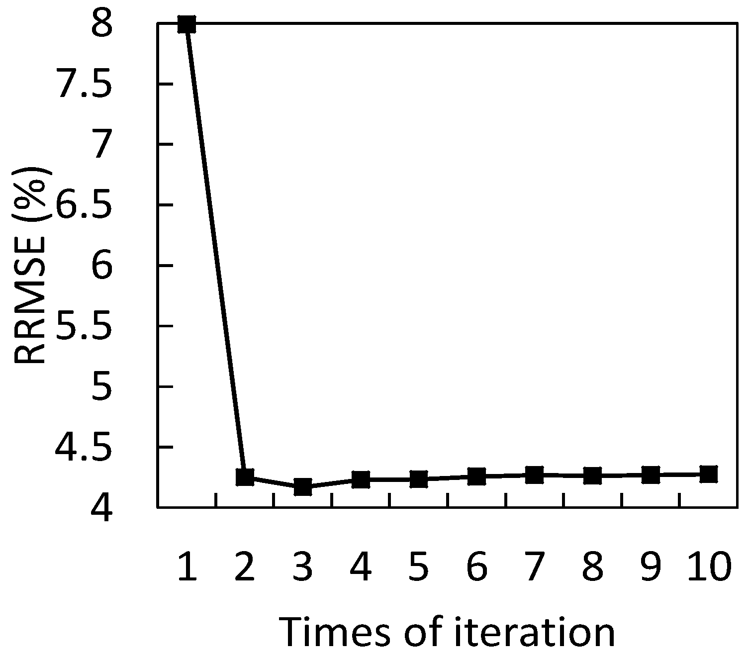
- (4)
- Remove the estimated SIF spectrum from the total upwelling radiance and then calculate a new apparent reflectance ; go back to steps (2) and (3) to reconstruct a new SIF spectrum .
- (5)
- Iterate until the reconstructed SIF spectrum is stable and then let SIF(λ) equal .

3. Results
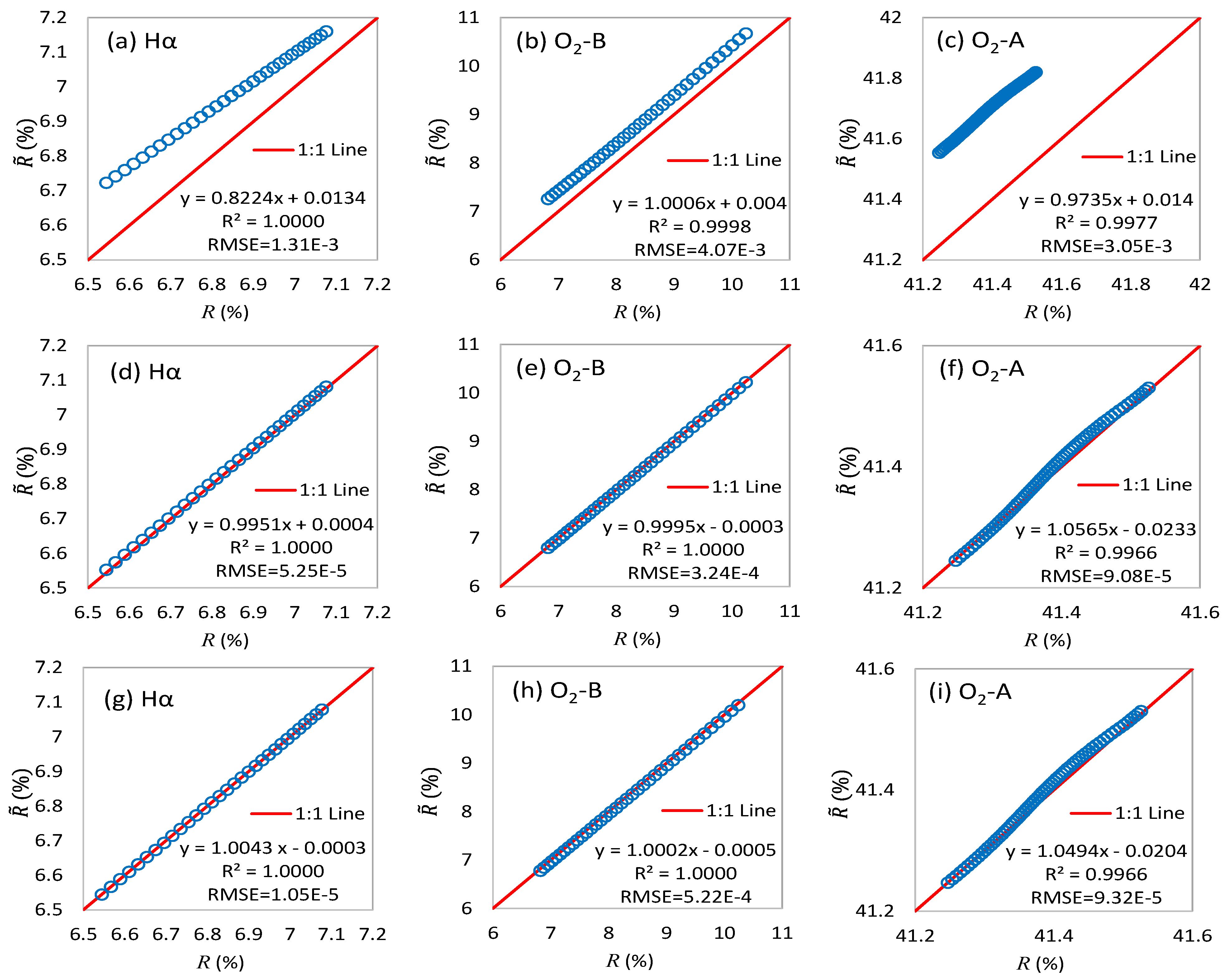
3.1. Accuracy Assessment with the Simulated Dataset


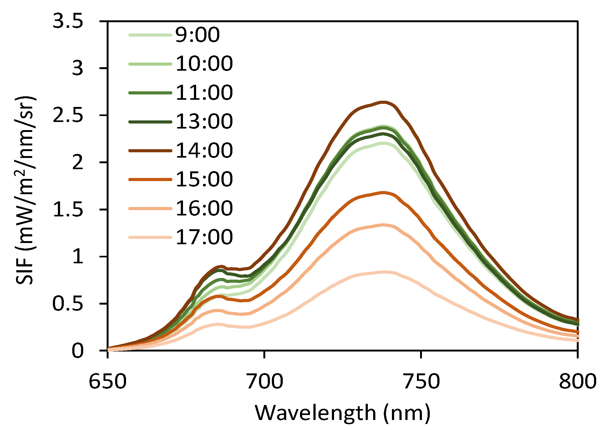
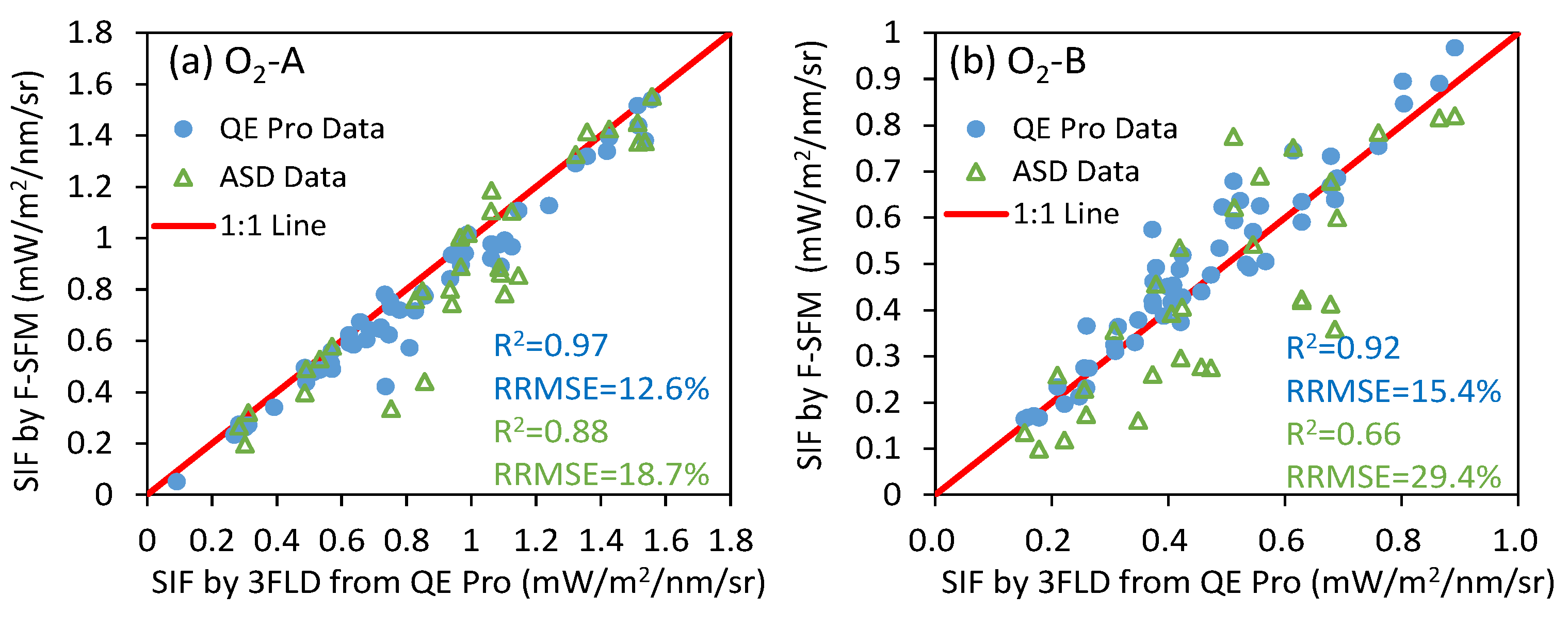
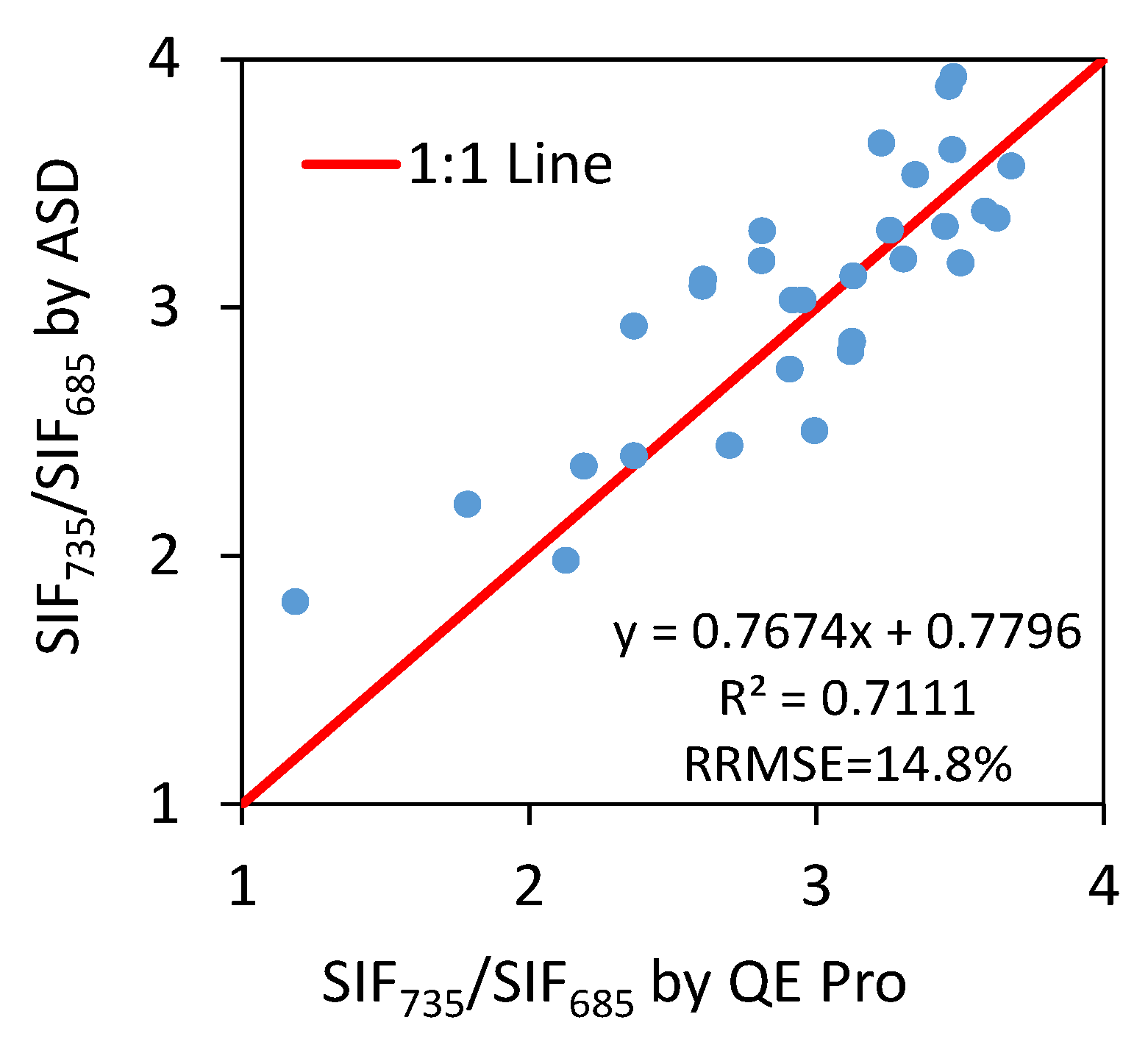
3.2. Testing of the Field-Measured Data


4. Discussion
4.1. Advantages of the Proposed F-SFM Algorithm
4.2. Limitations of the Proposed Method
5. Conclusions
Acknowledgments
Author Contributions
Conflicts of Interest
References
- Zarco-Tejada, P.J. Hyperspectral Remote Sensing of Closed Forest Canopies: Estimation of Chlorophyll Fluorescence and Pigment Content. Ph.D. Thesis, York University Toronto, Toronto, ON, Canada, December 2000. [Google Scholar]
- Baker, N.R. Chlorophyll fluorescence: A probe of photosynthesis in vivo. Annu. Rev. Plant Biol. 2008, 59, 89–113. [Google Scholar] [CrossRef] [PubMed]
- Meroni, M.; Rossini, M.; Guanter, L.; Alonso, L.; Rascher, U.; Colombo, R.; Moreno, J. Remote sensing of solar-induced chlorophyll fluorescence: Review of methods and applications. Remote Sens. Environ. 2009, 113, 2037–2051. [Google Scholar] [CrossRef]
- Gamon, J.; Penuelas, J.; Field, C. A narrow-waveband spectral index that tracks diurnal changes in photosynthetic efficiency. Remote Sens. Environ. 1992, 41, 35–44. [Google Scholar] [CrossRef]
- Suárez, L.; Zarco-Tejada, P.J.; Berni, J.A.; González-Dugo, V.; Fereres, E. Modelling pri for water stress detection using radiative transfer models. Remote Sens. Environ. 2009, 113, 730–744. [Google Scholar] [CrossRef]
- Zarco-Tejada, P.J.; Catalina, A.; González, M.R.; Martín, P. Relationships between net photosynthesis and steady-state chlorophyll fluorescence retrieved from airborne hyperspectral imagery. Remote Sens. Environ. 2013, 136, 247–258. [Google Scholar] [CrossRef]
- Meroni, M.; Picchi, V.; Rossini, M.; Cogliati, S.; Panigada, C.; Nali, C.; Lorenzini, G.; Colombo, R. Leaf level early assessment of ozone injuries by passive fluorescence and photochemical reflectance index. Inter. J. Remote Sens. 2008, 29, 5409–5422. [Google Scholar] [CrossRef]
- Ni, Z.; Liu, Z.; Huo, H.; Li, Z.-L.; Nerry, F.; Wang, Q.; Li, X. Early water stress detection using leaf-level measurements of chlorophyll fluorescence and temperature data. Remote Sens. 2015, 7, 3232–3249. [Google Scholar] [CrossRef]
- Delalieux, S.; Somers, B.; Verstraeten, W.; Van Aardt, J.; Keulemans, W.; Coppin, P. Hyperspectral indices to diagnose leaf biotic stress of apple plants, considering leaf phenology. Int. J. Remote Sens. 2009, 30, 1887–1912. [Google Scholar] [CrossRef]
- Berry, J.A.; Frankenberg, C.; Wennberg, P.; Baker, I.; Bowman, K.W.; Castro-Contreas, S.; Cendrero-Mateo, M.P.; Damm, A.; Drewry, D.; Ehlmann, B. New methods for measurement of photosynthesis from space. Geophys. Res. Lett. 2012, 38, L17706. [Google Scholar]
- Cheng, Y.-B.; Middleton, E.; Zhang, Q.; Huemmrich, K.; Campbell, P.; Corp, L.; Cook, B.; Kustas, W.; Daughtry, C. Integrating solar induced fluorescence and the photochemical reflectance index for estimating gross primary production in a cornfield. Remote Sens. 2013, 5, 6857–6879. [Google Scholar] [CrossRef]
- Lee, J.E.; Frankenberg, C.; van der Tol, C.; Berry, J.A.; Guanter, L.; Boyce, C.K.; Fisher, J.B.; Morrow, E.; Worden, J.R.; Asefi, S.; et al. Forest productivity and water stress in amazonia: Observations from gosat chlorophyll fluorescence. Roy. Soc. London B: Biol. Sci. 2013. [Google Scholar] [CrossRef]
- Damm, A.; Elbers, J.A.N.; Erler, A.; Gioli, B.; Hamdi, K.; Hutjes, R.; Kosvancova, M.; Meroni, M.; Miglietta, F.; Moersch, A.; et al. Remote sensing of sun-induced fluorescence to improve modeling of diurnal courses of gross primary production (gpp). Global Change Biol. 2010, 16, 171–186. [Google Scholar] [CrossRef] [Green Version]
- Zhang, Y.; Guanter, L.; Berry, J.A.; Joiner, J.; van der Tol, C.; Huete, A.; Gitelson, A.; Voigt, M.; Kohler, P. Estimation of vegetation photosynthetic capacity from space-based measurements of chlorophyll fluorescence for terrestrial biosphere models. Global Change Biol. 2014, 20, 3727–3742. [Google Scholar] [CrossRef] [PubMed]
- Pedrós, R.; Moya, I.; Goulas, Y.; Jacquemoud, S. Chlorophyll fluorescence emission spectrum inside a leaf. Photoch. Photobio. Sci. 2008, 7, 498–502. [Google Scholar] [CrossRef] [PubMed]
- Zarco-Tejada, P.J.; Miller, J.R.; Mohammed, G.H.; Noland, T.L.; Sampson, P.H. Chlorophyll fluorescence effects on vegetation apparent reflectance: Ii. Laboratory and airborne canopy-level measurements with hyperspectral data. Remote Sens. Environ. 2000, 74, 596–608. [Google Scholar] [CrossRef]
- Pfündel, E. Estimating the contribution of photosystem i to total leaf chlorophyll fluorescence. Photo. Res. 1998, 56, 185–195. [Google Scholar] [CrossRef]
- Agati, G.; Cerovic, Z.G.; Moya, I. The effect of decreasing temperature up to chilling values on the in vivo f685/f735 chlorophyll fluorescence ratio in phaseolus vulgaris and pisum sativum: The role of the photosystem i contribution to the 735 nm fluorescence band. Photoch. Photobio. 2000, 72, 75–84. [Google Scholar] [CrossRef]
- Krause, G.H.; Weis, E. Chlorophyll fluorescence and photosynthesis—the basics. Ann. Rev. Plant Biol. 1991, 42, 313–349. [Google Scholar] [CrossRef]
- Porcar-Castell, A.; Tyystjärvi, E.; Atherton, J.; van der Tol, C.; Flexas, J.; Pfündel, E.E.; Moreno, J.; Frankenberg, C.; Berry, J.A. Linking chlorophyll a fluorescence to photosynthesis for remote sensing applications: Mechanisms and challenges. J. Exp. Bot. 2014, eru191. [Google Scholar] [CrossRef] [PubMed]
- Gitelson, A.A.; Buschmann, C.; Lichtenthaler, H.K. Leaf chlorophyll fluorescence corrected for re-absorption by means of absorption and reflectance measurements. J. Plant Phys. 1998, 152, 283–296. [Google Scholar] [CrossRef]
- Lichtenthaler, H.K.; Rinderle, U. The role of chlorophyll fluorescence in the detection of stress conditions in plants. Crc. Crit. Rev. Anal. Chem. 1988, 19, S29–S85. [Google Scholar] [CrossRef]
- Plascyk, J.A. The mk ii fraunhofer line discriminator (fld-ii) for airborne and orbital remote sensing of solar-stimulated luminescence. Opt. Eng. 1975, 14, 339–346. [Google Scholar] [CrossRef]
- Plascyk, J.A.; Gabriel, F.C. Fraunhofer line discriminator mk ii—airborne instrument for precise and standardized ecological luminescence measurement. IEEE Trans. Instrum. Meas. 1975, 24, 306–313. [Google Scholar] [CrossRef]
- Maier, S.W.; Günther, K.P.; Stellmes, M. Sun-induced fluorescence: A new tool for precision farming. In Digital Imaging and Spectral Techniques: Applications to Precision Agriculture and Crop Physiology; McDonald, M., Schepers, J., Tartly, L., Toai, T.V., Major, D., Eds.; American Society of Agronomy Special Publication: Madison, WI, USA, 2003; pp. 209–222. [Google Scholar]
- Alonso, L.; Gomez-Chova, L.; Vila-Frances, J.; Amoros-Lopez, J.; Guanter, L.; Calpe, J.; Moreno, J. Improved fraunhofer line discrimination method for vegetation fluorescence quantification. IEEE Geosci. Remote Sens. Lett. 2008, 5, 620–624. [Google Scholar] [CrossRef]
- Meroni, M.; Colombo, R. Leaf level detection of solar induced chlorophyll fluorescence by means of a subnanometer resolution spectroradiometer. Remote Sens. Environ. 2006, 103, 438–448. [Google Scholar] [CrossRef]
- Meroni, M.; Busetto, L.; Colombo, R.; Guanter, L.; Moreno, J.; Verhoef, W. Performance of spectral fitting methods for vegetation fluorescence quantification. Remote Sens. Environ. 2010, 114, 363–374. [Google Scholar] [CrossRef]
- Mazzoni, M.; Falorni, P.; Verhoef, W. High-resolution methods for fluorescence retrieval from space. Opt. Express 2010, 18, 15649–15663. [Google Scholar] [CrossRef] [PubMed]
- Cogliati, S.; Rossini, M.; Schickling, A.; Pinto, F.; Alonso, L.; Vicent, J.; Sabater, N.; Colombo, R.; Rascher, U.; Verhoef, W.; et al. Retrieval of sun induced fluorescence using advanced spectral fitting methods from radiative transfer simulations and hyplant imagery. In Proceedings of the 5th International. Workshop on Remote Sensing of Vegetation Fluorescence, Paris, France, 22–24 April 2014.
- Zhao, F.; Guo, Y.; Verhoef, W.; Gu, X.; Liu, L.; Yang, G. A method to reconstruct the solar-induced canopy fluorescence spectrum from hyperspectral measurements. Remote Sens. 2014, 6, 10171–10192. [Google Scholar] [CrossRef]
- Liu, X.; Liu, L. Improving chlorophyll fluorescence retrieval using reflectance reconstruction based on principal components analysis. IEEE Geosci. Remote Sens. Lett. 2015, 12, 1645–1649. [Google Scholar] [CrossRef]
- Van der Tol, C.; Verhoef, W.; Timmermans, J.; Verhoef, A.; Su, Z. An integrated model of soil-canopy spectral radiances, photosynthesis, fluorescence, temperature and energy balance. Biogeosciences 2009, 6, 3109–3129. [Google Scholar] [CrossRef]
- Hosgood, J. The JRC Leaf Optical Properties EXperiment (LOPEX’'93) Report Eur-16096-en; European Commission Joint Research Centre: Ispra, Italy, 1995. [Google Scholar]
- Berk, A.; Anderson, G.P.; Acharya, P.K.; Bernstein, L.S.; Muratov, L.; Lee, J.; Fox, M.; Adler-Golden, S.M.; Chetwynd, J.H.; Hoke, M.L.; et al. Modtran (TM) 5, a reformulated atmospheric band model with auxiliary species and practical multiple scattering options: Update. In Algorithms and Technologies for Multispectral, Hyperspectral, and Ultraspectral Imagery XI; Shen, S.S., Lewis, P.E., Eds.; SPIE: Bellingham, WA, USA, 2005; Volume 5806, pp. 662–667. [Google Scholar]
- Verhoef, W.; van der Tol, C.; Middleton, E.M. Vegetation canopy fluorescence and reflectance retrieval by model inversion using optimization. Presented at the 5th International Workshop on Remote Sensing of Vegetation Fluorescence; Paris, French, 22–24 April 2014. [Google Scholar]
- Liu, X.; Liu, L. Assessing band sensitivity to atmospheric radiation transfer for space-based retrieval of solar-induced chlorophyll fluorescence. Remote Sens. 2014, 6, 10656–10675. [Google Scholar] [CrossRef]
- Damm, A.; Erler, A.; Hillen, W.; Meroni, M.; Schaepman, M.E.; Verhoef, W.; Rascher, U. Modeling the impact of spectral sensor configurations on the fld retrieval accuracy of sun-induced chlorophyll fluorescence. Remote Sens. Environ. 2011, 115, 1882–1892. [Google Scholar] [CrossRef]
- Hawkins, T.S.; Gardiner, E.S.; Comer, G.S.; Hawkins, T.S.; Comer, G.S. Modeling the relationship between extractable chlorophyll and spad-502 readings for endangered plant species research. J. Nat. Conserv. 2009, 17, 123–127. [Google Scholar] [CrossRef]
- Amoros-Lopez, J.; Gomez-Chova, L.; Vila-Frances, J.; Alonso, L.; Calpe, J.; Moreno, J.; del Valle-Tascon, S. Evaluation of remote sensing of vegetation fluorescence by the analysis of diurnal cycles. Int. J. Remote Sens. 2008, 29, 5423–5436. [Google Scholar] [CrossRef]
- Yang, X.; Tang, J.; Mustard, J.F.; Lee, J.E.; Rossini, M.; Joiner, J.; Munger, J.W.; Kornfeld, A.; Richardson, A.D. Solar-induced chlorophyll fluorescence correlates with canopy photosynthesis on diurnal and seasonal scales in a temperate deciduous forest. Geophys. Res. Lett. 2015, 42, 2977–2987. [Google Scholar] [CrossRef]
- Cogliati, S.; Rossini, M.; Julitta, T.; Meroni, M.; Schickling, A.; Burkart, A.; Pinto, F.; Rascher, U.; Colombo, R. Continuous and long-term measurements of reflectance and sun-induced chlorophyll fluorescence by using novel automated field spectroscopy systems. Remote Sens. Environ. 2015, 164, 270–281. [Google Scholar] [CrossRef]
© 2015 by the authors; licensee MDPI, Basel, Switzerland. This article is an open access article distributed under the terms and conditions of the Creative Commons Attribution license (http://creativecommons.org/licenses/by/4.0/).
Share and Cite
Liu, X.; Liu, L.; Zhang, S.; Zhou, X. New Spectral Fitting Method for Full-Spectrum Solar-Induced Chlorophyll Fluorescence Retrieval Based on Principal Components Analysis. Remote Sens. 2015, 7, 10626-10645. https://0-doi-org.brum.beds.ac.uk/10.3390/rs70810626
Liu X, Liu L, Zhang S, Zhou X. New Spectral Fitting Method for Full-Spectrum Solar-Induced Chlorophyll Fluorescence Retrieval Based on Principal Components Analysis. Remote Sensing. 2015; 7(8):10626-10645. https://0-doi-org.brum.beds.ac.uk/10.3390/rs70810626
Chicago/Turabian StyleLiu, Xinjie, Liangyun Liu, Su Zhang, and Xianfeng Zhou. 2015. "New Spectral Fitting Method for Full-Spectrum Solar-Induced Chlorophyll Fluorescence Retrieval Based on Principal Components Analysis" Remote Sensing 7, no. 8: 10626-10645. https://0-doi-org.brum.beds.ac.uk/10.3390/rs70810626