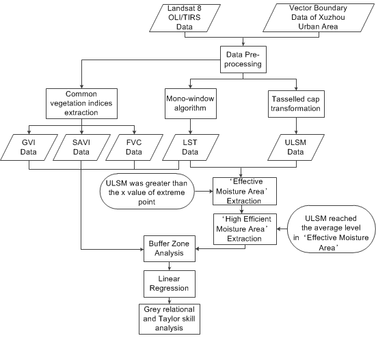
3.3.1. Comparative Indicators Selection
Previous studies have shown that vegetation has a very important effect on land surface temperatures in urban areas [
12,
14,
20]. Latent heat exchange is higher in areas of urban regions with concentrated vegetation [
52]. Studies have shown that the fractional vegetation cover (FVC) index [
53], soil adjusted vegetation index (SAVI) [
54] and Greenness vegetation index (GVI) [
51] have a negative correlation relationship with the land surface temperature [
21,
22,
55]. Therefore, the effect of the influence of ULSM, FVC, SAVI and GVI on the land surface temperature is a question that needs to be further studied. The equation for FVC is shown as formula 10 (
PV), the equation for GVI is shown in
Table 3 (Greenness), and the algorithm for SAVI [
21] is as follows.
where ρ
nir is near red band reflectance (band 5), ρ
red is red band reflectance (band 4) and L is an adjustment factor, set to minimum background effects (L = 0.5).
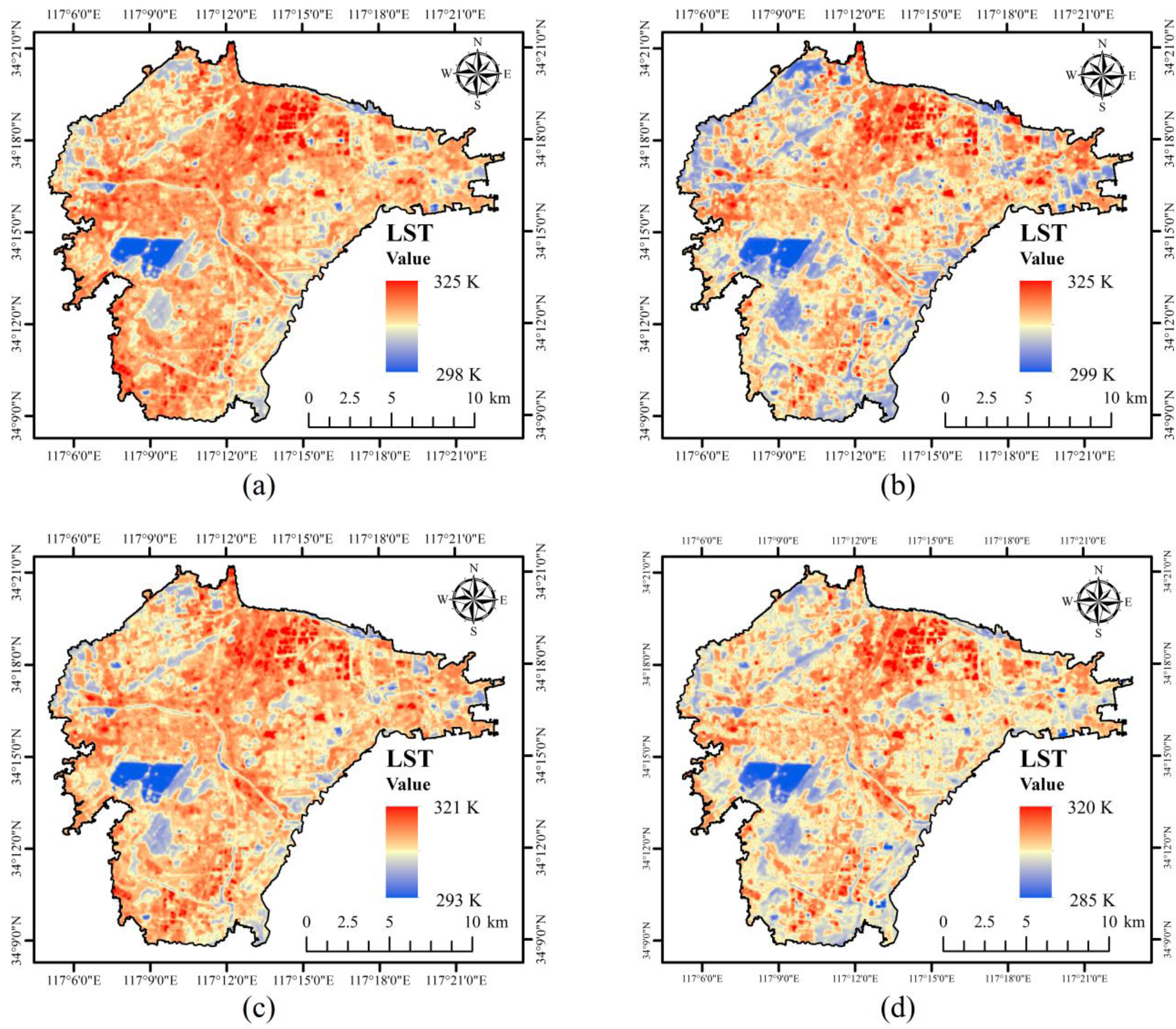
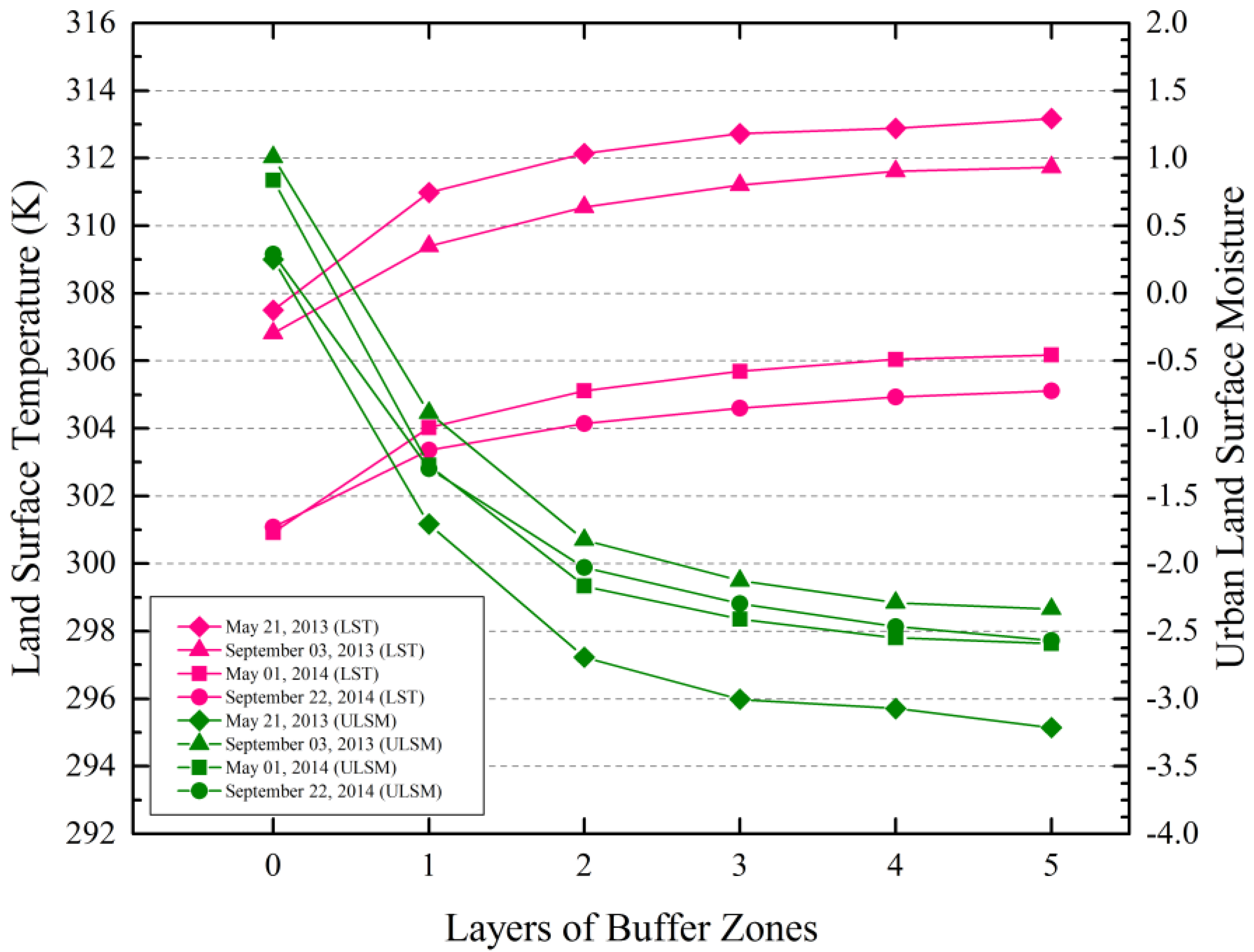
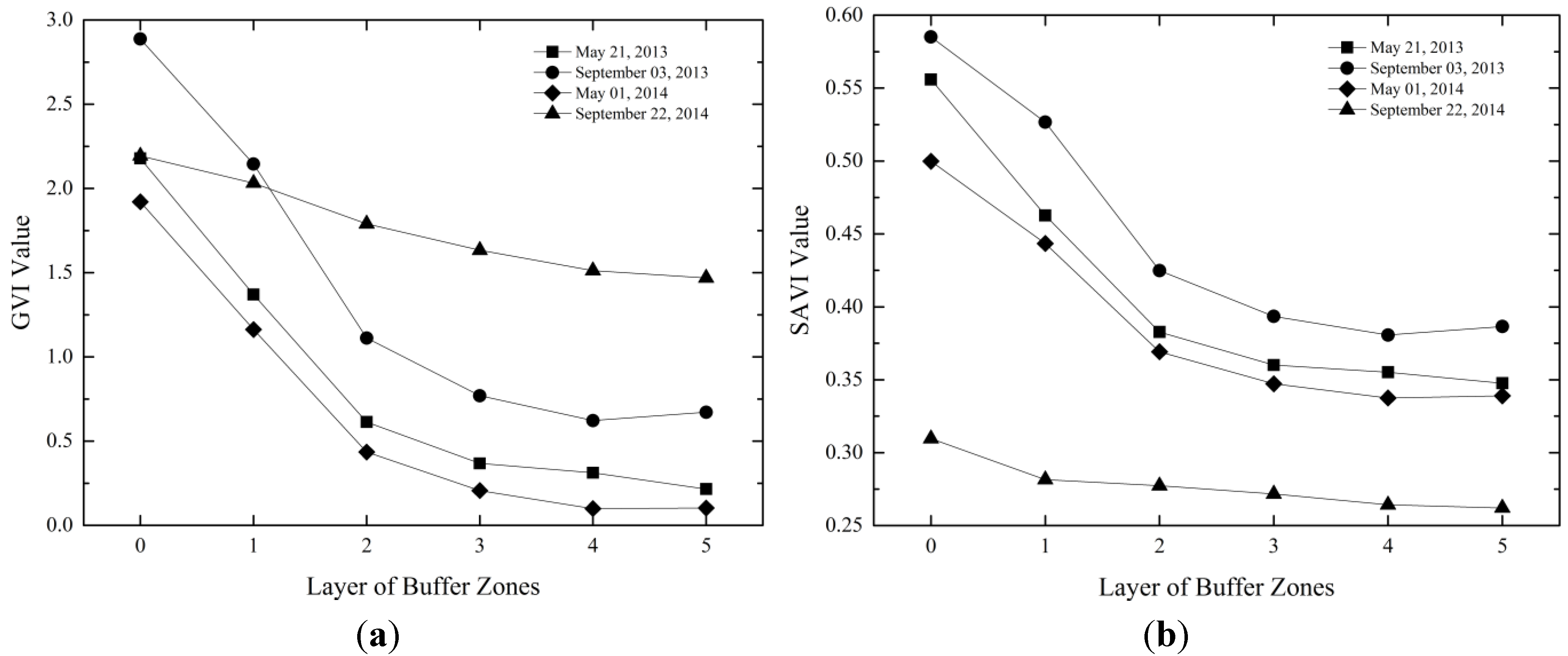
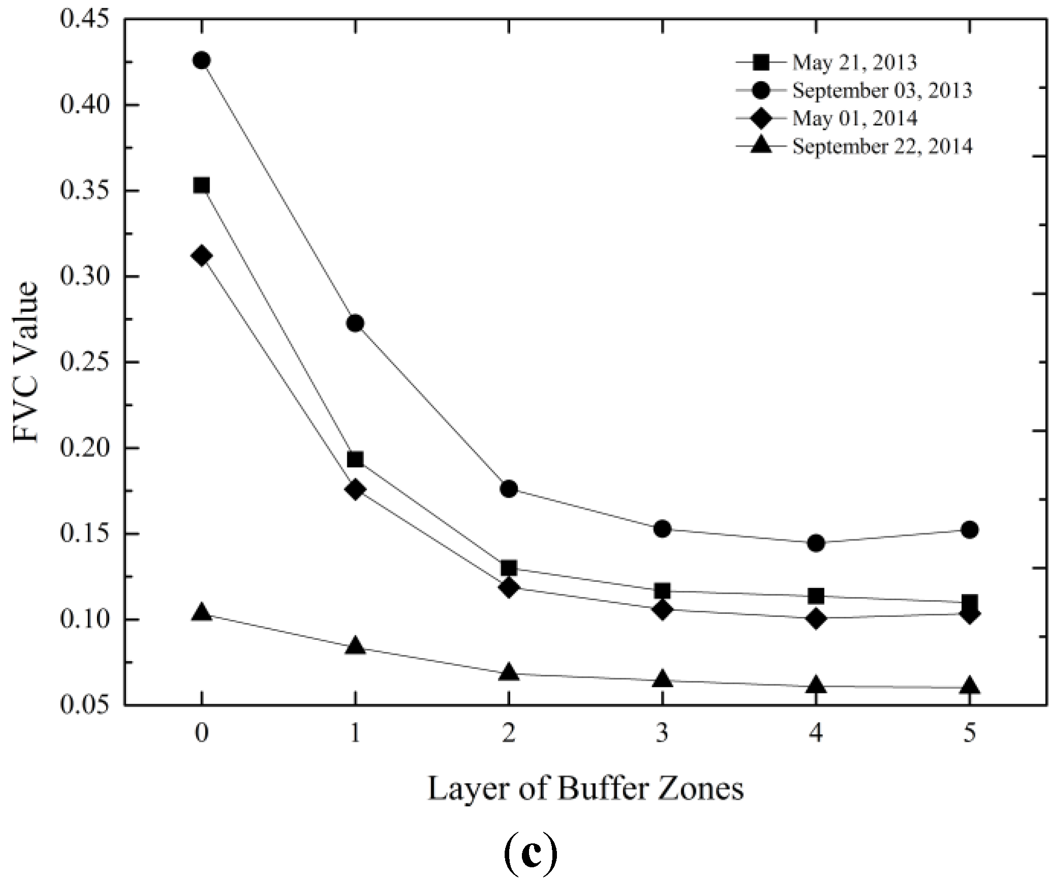
Figure 9 shows that on the whole, GVI, SAVI and FVC decrease as the distance increases from the core areas. The value changes of GVI, SAVI and FVC compared with the changes of the land surface temperature in each layer of the buffer zones were basically the opposite.
Figure 9.
(a) GVI average value in the core areas and each layer of the buffer zones; (b) SAVI average value in the core areas and each layer of the buffer zones; (c) FVC average value in the core areas and each layer of the buffer zones. The zero points on the x axis refers to core areas.
Figure 9.
(a) GVI average value in the core areas and each layer of the buffer zones; (b) SAVI average value in the core areas and each layer of the buffer zones; (c) FVC average value in the core areas and each layer of the buffer zones. The zero points on the x axis refers to core areas.
3.3.2. Indices Normalized and Univariate Linear Regression Analysis
After the GVI, SAVI and FVC average values of the core areas and each layer of the buffer zones were extracted, the declining value of these three indices in each layer were calculated using the inner average value minus the outer average value in turn from the core areas to the last layer of the buffer zones. To compare the influence of the four indices on the land surface temperatures of the surrounding areas, normalized processing was used to eliminate the influence of the magnitude order. For instance, normalized processing of the SAVI declining value was as follows.
SAVID is the declining value of SAVI, SAVID
N is the normalized processing value of SAVID, SAVID
MIN is the minimum value of SAVID and SAVID
MAX is the minimum value of SAVID. The normalized processing declining value of ULSM, GVI, SAVI, and FVC and the increasing value of LST are shown in
Table 7.
Table 7.
The normalized processing value of ULSMD, GVID, SAVID, FVCD and LSTI. C refers to core area, Li (i = 1,2,3,4,5) refer to each layer of buffer zones.
Table 7.
The normalized processing value of ULSMD, GVID, SAVID, FVCD and LSTI. C refers to core area, Li (i = 1,2,3,4,5) refer to each layer of buffer zones.
| Index | 21 May 2013 | 03 September 2013 |
|---|
| C-L1 | L1-L2 | L2-L3 | L3-L4 | L4-L5 | C-L1 | L1-L2 | L2-L3 | L3-L4 | L4-L5 |
|---|
| ULSMDN | 0.9274 | 0.4549 | 0.1303 | 0.0121 | 0.0473 | 0.8956 | 0.4340 | 0.1253 | 0.0582 | 0.0019 |
| GVIDN | 0.7923 | 0.7452 | 0.2729 | 0.0975 | 0.1350 | 0.7319 | 1.0000 | 0.3620 | 0.1822 | 0.0000 |
| SAVIDN | 0.9207 | 0.7970 | 0.2640 | 0.0990 | 0.1237 | 0.5966 | 1.0000 | 0.3456 | 0.1718 | 0.0000 |
| FVCDN | 1.0000 | 0.4240 | 0.1257 | 0.0645 | 0.0680 | 0.9605 | 0.6231 | 0.1853 | 0.0960 | 0.0000 |
| LSTIN | 1.0000 | 0.3048 | 0.1382 | 0.0075 | 0.0485 | 0.7290 | 0.3086 | 0.1564 | 0.0814 | 0.0000 |
| Index | 01 May 2014 | 22 September 2014 |
| C-L1 | L1-L2 | L2-L3 | L3-L4 | L4-L5 | C-L1 | L1-L2 | L2-L3 | L3-L4 | L4-L5 |
| ULSMDN | 1.0000 | 0.4129 | 0.0971 | 0.0463 | 0.0000 | 0.7473 | 0.3324 | 0.1091 | 0.0618 | 0.0286 |
| GVIDN | 0.7463 | 0.7175 | 0.2576 | 0.1445 | 0.0431 | 0.1951 | 0.2691 | 0.1907 | 0.1578 | 0.0869 |
| SAVIDN | 0.5781 | 0.7439 | 0.2583 | 0.1439 | 0.0392 | 0.3146 | 0.0920 | 0.1058 | 0.1224 | 0.0734 |
| FVCDN | 0.8599 | 0.3868 | 0.1235 | 0.0772 | 0.0288 | 0.1631 | 0.1381 | 0.0696 | 0.0664 | 0.0490 |
| LSTIN | 0.8840 | 0.2858 | 0.1342 | 0.0681 | 0.0007 | 0.6386 | 0.1961 | 0.1004 | 0.0592 | 0.0182 |
Univariate linear regression analysis was used between LSTI
N and ULSM
N, GVI
N, SAVI
N, and FVCD
N. The results of the regression analysis are shown in
Figure 10 and
Table 8.
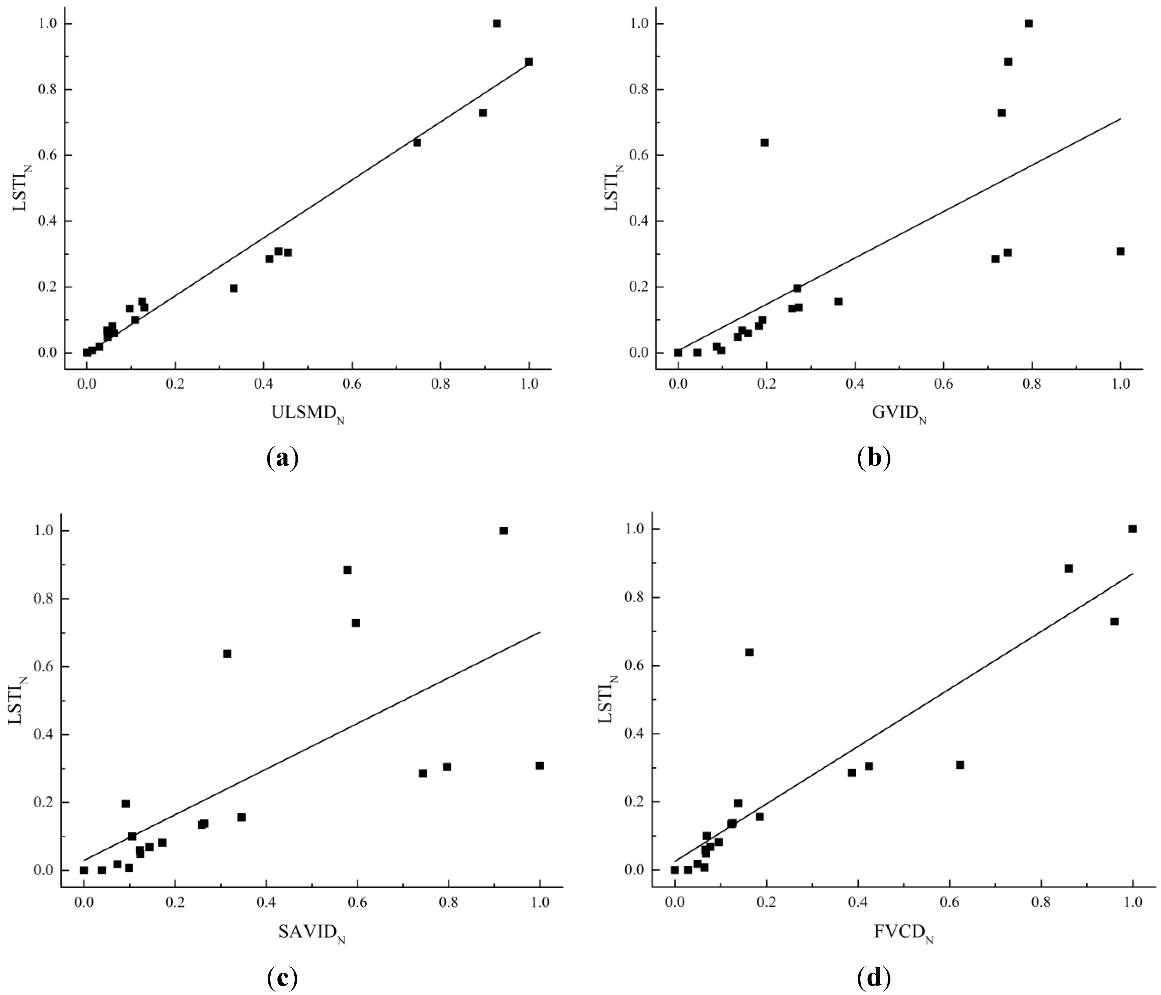
Figure 10.
(a) Linear regression between LSTIN and ULSMDN; (b) Linear regression between LSTIN and GVIDN; (c) Linear regression between LSTIN and SAVIDN; (d) Linear regression between LSTIN and FVCDN.
Figure 10.
(a) Linear regression between LSTIN and ULSMDN; (b) Linear regression between LSTIN and GVIDN; (c) Linear regression between LSTIN and SAVIDN; (d) Linear regression between LSTIN and FVCDN.
Table 8.
Result of regression analysis between LSTIN and ULSMDN, GVIDN, SAVIDN, FVCDN.
Table 8.
Result of regression analysis between LSTIN and ULSMDN, GVIDN, SAVIDN, FVCDN.
| Index | Correlation Coefficient | Regression Equation | RMSE | P-Value |
|---|
| LSTIN vs. ULSMDN | 0.9790 | y1 = 0.8804 x1 − 0.0027 | 0.0642 | 6.99 × 10⁻¹⁴ < 0.05 |
| LSTIN vs. GVIDN | 0.7031 | y2 = 0.7035 x2 + 0.0073 | 0.2240 | 5.44 × 10⁻⁴ < 0.05 |
| LSTIN vs. SAVIDN | 0.6921 | y3 = 0.6725 x3 + 0.0297 | 0.2274 | 7.21 × 10⁻⁴ < 0.05 |
| LSTIN vs. FVCDN | 0.8939 | y4 = 0.8430 x4 + 0.0256 | 0.1412 | 1.09 × 10⁻⁷ < 0.05 |
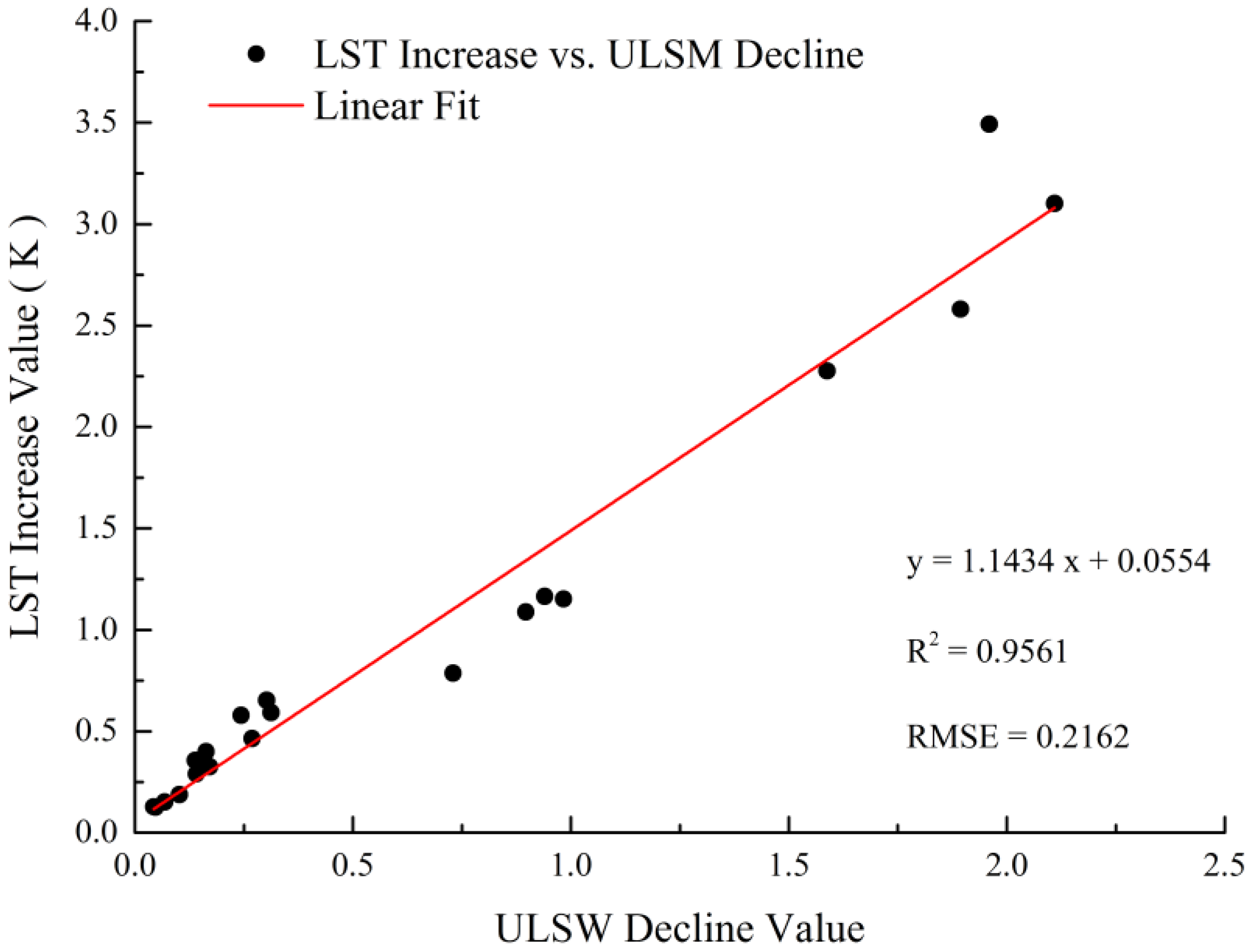
It can be seen from
Figure 10 and
Table 8 that these four indices all have significant linear positive correlation with LSTI
N within the confidence interval of 95%. In addition, LSTI
N and ULSMD
N have the best fitting effect with the highest correlation coefficient value of 0.9790 and the lowest RMSE value of 0.0642. On the other hand, LSTI
N and SAVID
N have a poor fitting effect, with a lowest correlation coefficient value of 0.6921 and a highest RMSE value of 0.2274 compared with the other three indices. The univariate regression analysis reveals that the change of ULSM has a high correlation with the change of the land surface temperature in the surrounding areas.
3.3.3. Grey Relational and Taylor Skill Analysis
The fact that the declining value of ULSM had a higher correlation with the increasing value of the land surface temperature cannot statistically prove that the ULSM is more important than other indices of GVI, SAVI and FVC. Therefore, grey relational analysis was chosen for multi-factor correlation analysis.
Grey relational analysis was first put forward by Julong Deng [
56]. It is applied to measure the correlation degree between different factors based on similarity in the developing trends of these factors. Because the increasing value of the LST and the declining value of ULSM, GVI, SAVI and FVC have linear positive relationships, grey relational analysis was thought to be very suitable for calculating the various influence degrees of ULSM, GVI, SAVI, and FVC on land surface temperature changes. According to the regression equation in
Table 6, the LSTI
N predicted values (
y1,
y2,
y3,
y4) were calculated through ULSMD
N (
x1), GVID
N (
x2), SAVID
N (
x3) and FVCD
N (
x4), and then, 20 predicted data points for each index were exported in the order of time and buffer hierarchy (
Figure 11).
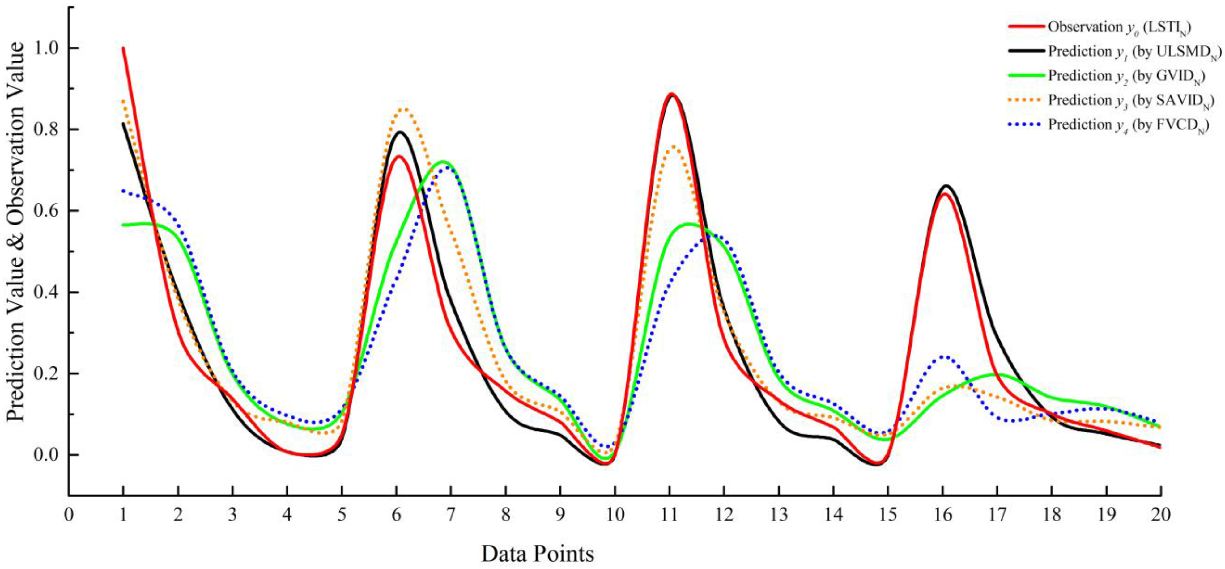
The variation trend of the ULSMD
N predicted value was closest to the variation trend of the LSTI normalized index compared to the predicted value of the other three indices. In the theory of grey relational analysis, the correlation degree is in essence the difference of the geometric shape between different curves. Thus, the difference between different curves can be used to measure the relation degree. For instance, in
Figure 11, for
x = 1, when the values of
y0(1),
y1(1),
y2(1),
y3(1), and
y4(1) are obtained, the difference between
y0(1) and
yi(1) (i = 1,2,3,4) can be described as the difference between curve 0 and curve
i at x = 1. For a standard data array
y0 with several comparison data arrays
y1,
y2, …,
yn, the association coefficient ξ
(yi) between the standard data array and each comparison data array in each moment (that is, each calibration on the x axis) can be calculated by the following formula.
Figure 11.
Change trends of the LSTIN predicted value and the LSTIN observation value.
Figure 11.
Change trends of the LSTIN predicted value and the LSTIN observation value.
This formula gives the association coefficient of
yi for
y0 in k moment.
y0(k) refers to LSTI
N;
yi(k) (
i = 1,2,3,4) refers to the predicted value of LSTI
N calculated by ULSMD
N, GVID
N, SAVID
N and FVCD
N;
k refers to each point in the curve (
k = 1,2,3,…,20); and
ρ refers to the resolution coefficient, generally chosen as ρ = 0.5. The association coefficient of each data array in each moment has been shown in
Table 9.
Table 9.
The association coefficient of each data array.
Table 9.
The association coefficient of each data array.
| k | ξ1(k) | ξ2(k) | ξ3(k) | ξ4(k) |
|---|
| 1 | 0.5711 | 0.3626 | 0.4136 | 0.6541 |
| 2 | 0.7277 | 0.5223 | 0.4872 | 0.7605 |
| 3 | 0.9057 | 0.8032 | 0.7830 | 0.9763 |
| 4 | 0.9999 | 0.7846 | 0.7369 | 0.7741 |
| 5 | 0.9641 | 0.8229 | 0.7948 | 0.8788 |
| 6 | 0.8144 | 0.5453 | 0.4539 | 0.7000 |
| 7 | 0.7786 | 0.3812 | 0.3863 | 0.5055 |
| 8 | 0.8366 | 0.7019 | 0.7016 | 0.9079 |
| 9 | 0.8841 | 0.8219 | 0.7961 | 0.9087 |
| 10 | 0.9975 | 0.9730 | 0.8942 | 0.9071 |
| 11 | 0.9766 | 0.4133 | 0.3472 | 0.6505 |
| 12 | 0.7684 | 0.5228 | 0.5038 | 0.7903 |
| 13 | 0.8289 | 0.8213 | 0.7827 | 0.9843 |
| 14 | 0.8929 | 0.8597 | 0.8105 | 0.9175 |
| 15 | 0.9882 | 0.8715 | 0.8184 | 0.8348 |
| 16 | 0.9386 | 0.3339 | 0.3840 | 0.3426 |
| 17 | 0.7260 | 0.9998 | 0.7038 | 0.8221 |
| 18 | 0.9738 | 0.8592 | 1.0000 | 0.9409 |
| 19 | 0.9721 | 0.8085 | 0.8254 | 0.9180 |
| 20 | 0.9846 | 0.8326 | 0.8036 | 0.8362 |
| Average | 0.8765 | 0.7021 | 0.6714 | 0.8005 |
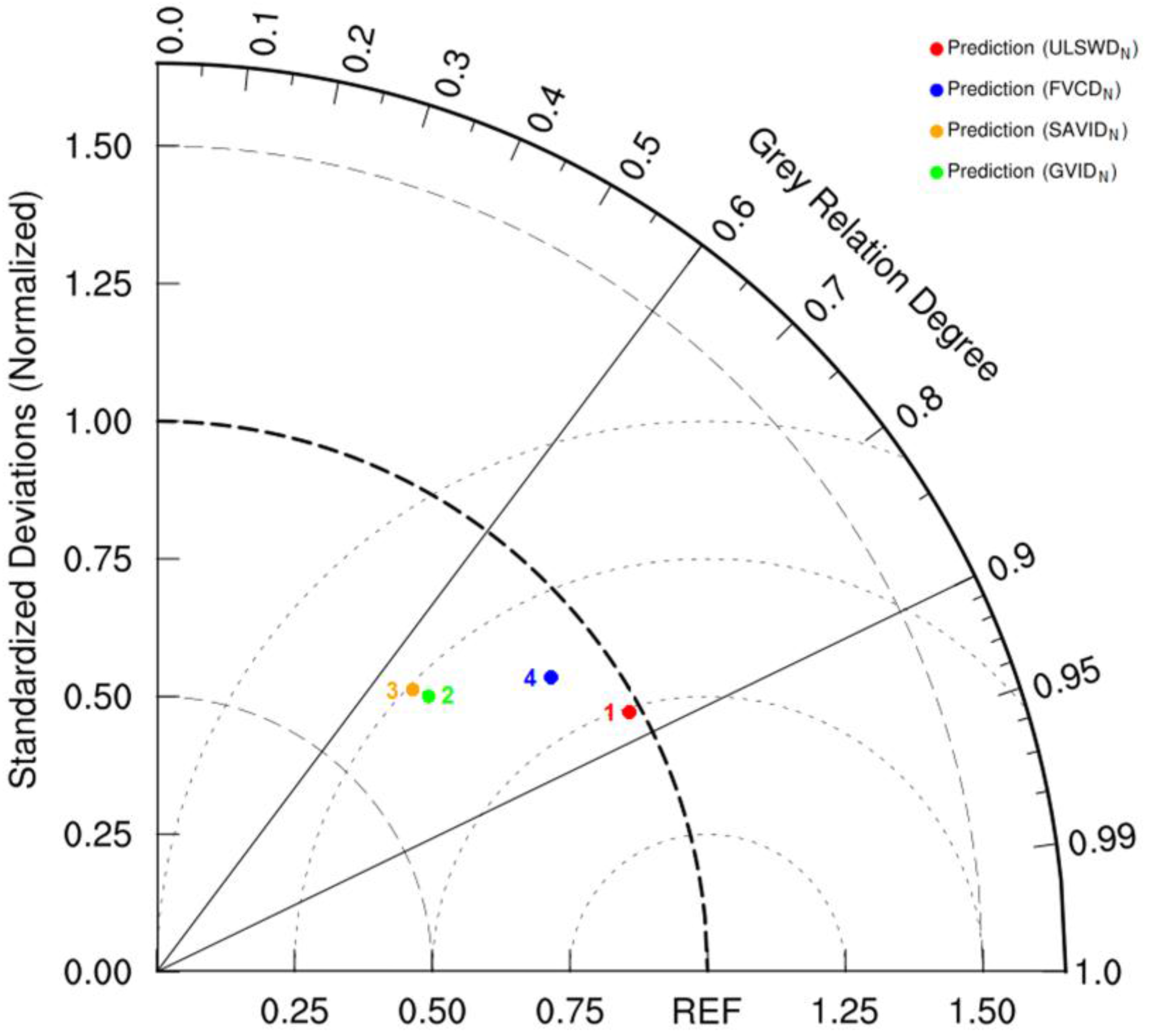
Finally, the relation degrees were derived by calculating the average value of the association coefficients of each data array. The performance of four types of predicted results are presented in an adjusted Taylor diagram (
Figure 12).
Figure 12.
Performance of the predicted values calculated by four indices (the statistics in the Taylor diagram); an ideal model would have a standard deviation ratio (σnorm) of 1.0 and a correlation coefficient of 1.0 (REF is the reference point).
Figure 12.
Performance of the predicted values calculated by four indices (the statistics in the Taylor diagram); an ideal model would have a standard deviation ratio (σnorm) of 1.0 and a correlation coefficient of 1.0 (REF is the reference point).
In this research, the Taylor diagram was adjusted by changing the correlation coefficient axis into a grey relation degree axis. A single point indicates the grey relation degree (
Rd = ξ) and the ratio of the standard deviations (σ) between the prediction (σ
p) and the observation (σ
o) (σ
norm = σ
p/σ
o). An ideal model would have a standard deviation ratio of 1.0 and a grey relation degree of 1.0,
i.e., the reference point (REF) on the x axis [
57]. Taylor skill (
S) is a single value summary of a Taylor diagram where unity indicates perfect agreement with observations. Traditionally, skill scores have been defined to vary from 0 (least skillful) to 1 (most skillful), each point for any arbitrary data group [
58,
59] can be scored as follows:
The calculation results of ξ, σ
norm, and
S are shown in
Table 10.
Table 10.
The association coefficient of each data array.
Table 10.
The association coefficient of each data array.
| Indicator | y1 | y2 | y3 | y4 |
|---|
| σnorm (σp/σo) | 0.9790 | 0.7031 | 0.6921 | 0.8939 |
| Rd (ξ) | 0.8765 | 0.7021 | 0.6714 | 0.8005 |
| Taylor skill (S) | 0.9378 | 0.7536 | 0.7320 | 0.8890 |


 ,
, 


